
A novel route to fabricate high-density graphene assemblies for high-volumetric-performance supercapacitors: effect of cation pre-intercalation†
Daoqing Liu,
Zheng Jia* and
Dianlong Wang
School of Chemical Engineering and Technology, Harbin Institute of Technology, Harbin 150001, China. E-mail: 13104059037@163.com
First published on 7th April 2016
Abstract
A simple procedure of cation pre-intercalation is incorporated with the ordinary graphene oxide thermal reduction method, readily producing graphene assemblies with a compact laminated structure and enhanced density, which exhibit anomalously high gravimetric capacitances and outstanding volumetric performances (a volumetric energy density of 26 W h L−1 in the aqueous electrolyte), primarily due to the contribution of ultramicropores.
1. Introduction
Supercapacitors are ideal high-power energy storage devices due to their fast response rate and long cycle life. Numerous porous carbon materials have been explored as supercapacitor electrode materials and their highly-developed porosity has been particularly pursued to provide large electric double layer (EDL) capacitance. Nevertheless, their overabundant pores unnecessarily occupy too much space, lowering the volumetric performances, which are actually of significant importance because the volume available for supercapacitors in a certain mobile device is always limited.As the building block of conductive carbon materials, graphene faces the contradiction between porosity and compactness as well, although it has good attributes suitable for supercapacitor electrodes including an excellent electrical conductivity and open pore structure.
Initially, the gravimetric specific surface area (SSA) value of graphene was believed as the most important parameter representing its porosity and predicting its EDL capacitance, thus had been enhanced as far as possible to approach its theoretical value (2630 m2 g−1). Accordingly, much effort has been devoted to prohibit the spontaneous firm aggregation (or called restacking) of graphene layers caused by the π–π attraction. One way for this purpose is the use of relatively harsh exfoliation conditions to produce well-separated graphene, including vacuum-promoted,1 microwave-assistant2 or high temperature3 thermal expansion, and laser scribing4 of graphite oxide. Another route is using “spacers”, such as carbon blacks,5 carbon nanotubes (CNTs),6 and water,7 inserted between graphene layers to construct tremendous interlayer pores. Besides, the chemical activation8 of graphene were explored to create additional in-plane pores to increase the graphene SSA. Nevertheless, the graphene materials prepared by the above methods seldom manifested acceptable volumetric performances, although their gravimetric performances did increase with their SSA value.
Gradually, the necessity of largely shrinking the pore size and hence pore volume meanwhile retaining appropriate SSA value to enhance the volumetric performances of graphene materials was recognized. Remarkable progresses have been made via various synthetic strategies, including the template-assisted fabrication of compact but still porous graphene,9,10 dense frameworks with single-layer graphene fragments in-between sheets,11 compactly interlinked graphene nanosheets produced by an evaporation-induced drying of a graphene hydrogel,12 liquid-mediated dense graphene films,13 and regular, compact but microporous graphene assemblies with intercalated potassium ions.14 Particularly, some certain high-density carbons were seemingly nonporous, but exhibited excellent supercapacitive behaviors, thus delivering high areal and volumetric capacitance. It was believed in one report that the abnormally high capacitance originated from the pseudo-capacitance induced by the nitrogen and fluorine co-doping,15 while the other reports attributed the high capacitance to the contribution of the commonly ignored ultramicropore.14,16 Therefore, such a peculiar capacitive phenomenon and its intrinsic regularity need further exploration.
The thermal reduction of graphite oxide is a routine graphene production method through decomposing oxygen-containing groups into gases, which quickly evolve to expand graphite oxide into extremely fluffy single graphene sheets.1,3 Herein, a simple procedure of cation pre-intercalation is coupled with the thermal reduction method, marvelously producing high-density graphene assemblies. The most interesting thing is that these thermally expanded graphene assemblies with high density exhibit anomalously high gravimetric capacitances and outstanding volumetric performances, which are thoroughly researched to disclose the fundamental mechanism on the basis of structure analyses and electrochemical measurements.
2. Experimental
2.1. Sample preparation
All of the reagents used are analytical grade without any further treatment before use. Graphite oxide was prepared from natural graphite (Xinghe Co., Qingdao, China) according to a modified Hummers method, as we previously reported.17,18500 mg graphite oxide was exfoliated into GO sheets and homogeneously dispersed in 500 mL distilled water through ultrasonication. 35.5 g Na2SO4 was added into the formed GO dispersion, which was stirred violently for 6 h. The flocculated dispersion was filtered and dried in air at 50 °C for 24 h. Then, the obtained aggregate was heated in air at a temperature ramp of 2 °C min−1 and kept at 200 °C for 1 h. The calcination product was washed with distilled water and filtered, and then dried. The finally obtained thermally expanded graphene is called TEGA-Na.
500 mg graphite oxide was exfoliated into GO sheets and homogeneously dispersed in 500 mL distilled water through ultrasonication. 37 g KCl was added into the formed GO dispersion, which was stirred violently for 6 h. The flocculated dispersion was filtered and dried in air at 50 °C for 24 h. Then, the obtained aggregate was thermally treated under the same conditions as TEGV. The calcination product was washed with distilled water and filtered, and then dried. The finally obtained thermally expanded graphene is called TEGV-K.
500 mg graphite oxide was exfoliated into GO sheets and homogeneously dispersed in 500 mL distilled water through ultrasonication. 37 mL concentrated HCl (37 wt%) was added into the formed GO dispersion, which was stirred violently for 6 h. The flocculated dispersion was filtered and dried in air at 50 °C for 24 h. Then, the obtained aggregate was thermally treated under the same conditions as TEGV. The calcination product was washed with distilled water and filtered, and then dried. The finally obtained thermally expanded graphene is called TEGV-H.
2.2. Sample characterization
The surface morphology and microstructure of samples were characterized by SEM with a Quanta 200FEG (FEI, American). N2 adsorption/desorption isotherms at −196 °C were measured with an ASAP2020 (Micromeritics, USA), and the corresponding SSA values and pore size distribution curves were obtained by Brunauer–Emmett–Teller (BET) and Barrett–Joyner–Halenda (BJH) analyses of the N2 adsorption isotherms, respectively. CO2 adsorption isotherms at 0 °C were measured using an Autosorb IQ (Quantachrome, USA), and the corresponding SSA values and pore size distribution curves were obtained by Density Functional Theory (DFT) analyses of the CO2 adsorption isotherms. X-ray diffraction (XRD) measurements were conducted using a D/max-γB system (Cu Kα radiation, λ = 0.154178 nm, XRD, Rigaku, Japan). Raman spectra were measured with a Renishaw inVia Raman spectrometer employing a 532 nm laser beam. Infrared spectra were measured on a Perkin-Elmer Spectrum 100 FT-IR Spectrometer in a frequency range of 4000–400 cm−1. X-ray photoelectron spectroscopy (XPS) measurements were performed with a K-Alpha (Thermofisher Scientific Company), which used an Al Kα monochromator.2.3. Electrochemical measurement
All the electrochemical measurements were carried out using CR2025 type symmetric supercapacitors in 30 wt% KOH or 1 mol L−1 Na2SO4 aqueous electrolyte or 1 mol L−1 Et4NBF4/AN organic electrolyte in a two-electrode configuration. Each electrode contained 80% the prepared graphene material, 10% conductive additive (acetylene black) and 10% polytetrafluoroethylene (PTFE), which were firstly mixed together in ethanol, and then rolled into sheets and punched into disks of 1.4 cm in diameter. After drying overnight at 75 °C under vacuum, the electrode disks were pressed onto nickel foam collectors to obtain electrodes. A pair of such electrodes with similar mass were chosen to assemble a supercapacitor, and the graphene mass loading per electrode is between 2.5 and 3.5 mg.The cyclic voltammetry (CV), electrochemical impedance spectroscopy (EIS) and galvanostatic charge/discharge tests were conducted using a CHI660E workstation (Chenhua, Shanghai, China).
From the CV curves, the gravimetric capacitances were calculated according the following equation:
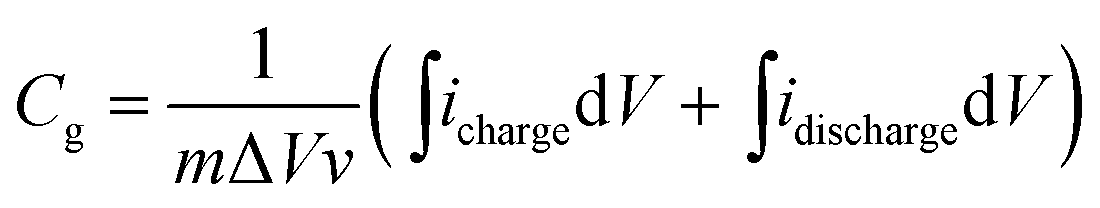 | (1) |
From the galvanostatic charge/discharge curves, the gravimetric capacitances were calculated by the following equation:
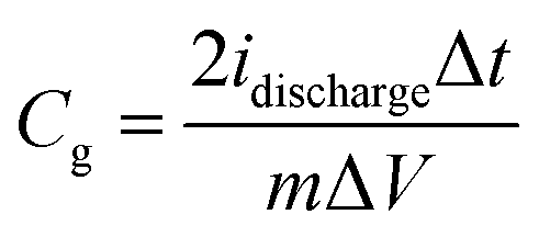 | (2) |
From the EIS plots, the gravimetric capacitances at different frequencies were calculated according to the following equation:
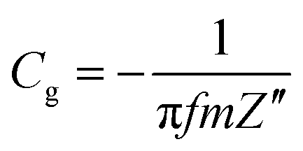 | (3) |
The volumetric capacitances were calculated using the following equation:
| Cv = ρCg | (4) |
The gravimetric and volumetric energy densities were calculated as follows:
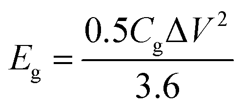 | (5) |
| Ev = ρEg | (6) |
The gravimetric and volumetric power densities were calculated according to the following equation:
 | (7) |
| Pv = ρPg | (8) |
3. Results and discussion
3.1. Morphology and microstructure
It can be seen from Fig. 1a that floccules are formed instantaneously after Na2SO4 is added into the GO suspension due to the coagulation of electrostatically screened GO layers caused by the adsorbed Na+ cations,19 which are subsequently left in the formed GO aggregates after desiccation as pre-intercalated specie. The same scenario is observed when KCl or HCl is added into the GO suspension, as shown in Fig. S8b (ESI†). The digital photos of the samples in Fig. 1b clearly indicates that TEGA-Na has a higher packing density than TEGA and TEGV, and this vivid observation is consistent with the density values calculated by two different methods, as listed in Table 2. Similarly, TEGV-K, TEGV-H and TEGV display a decreasing density order (Fig. S8c and Table S3, ESI†). Such a difference in density originates from various graphene stacking structures of the samples. The SEM images of TEGV, TEGA and TEGA-Na shown in Fig. 1c–e reveal their different morphologies and interlayer pore structures. Obviously, more large pores are observed in TEGV than TEGA because vacuum effect exerts an additional exfoliation force. Comparatively, TEGA-Na shows a compact laminated structure (see also Fig. S1a and b, ESI†), which indicates its lowest thermal expansion degree due to weak exfoliation pressure established between the loosely stacked layers of GO aggregates with pre-intercalated Na+ cations. The EDX spectrum (Fig. S2, ESI†) and XPS survey spectrum (Fig. S4b, ESI†) of TEGA-Na show that Na element does remain in TEGA-Na. Furthermore, the EDX elemental mappings in Fig. 1f reveal that Na element is relatively uniformly distributed in TEGA-Na.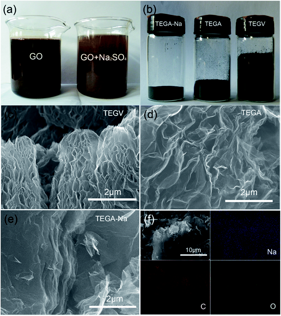 | ||
| Fig. 1 Digital photos of (a) the GO suspension before and after the addition of Na2SO4 and (b) the powders of TEGA-Na (0.2 g), TEGA (0.2 g) and TEGV (0.1 g). SEM images of (c) TEGV, (d) TEGA and (e) TEGA-Na. (f) EDX elemental mappings of TEGA-Na. | ||
The N2 adsorption/desorption isotherms in Fig. 2a reveal that the BET SSA value of TEGA-Na (84 m2 g−1) is much lower than TEGA (215 m2 g−1) and TEGV (271 m2 g−1) (Tables 1 and S3, ESI†), and the pore size (inset in Fig. 2a) and pore volume (Table 1) in the mesopore and large micropore range are largely shrunk for TEGA-Na. Accordingly, the percentage of micropores of TEGA-Na (68.8%) is much greater than TEGA (9.5%) (Table 1). The CO2 adsorption isotherms in Fig. 2b display that the SSA (175 m2 g−1) and pore volume (0.057 cm3 g−1) in the micropore range of TEGA-Na are also lower than those of TEGA (206 m2 g−1 and 0.070 cm3 g−1) (Table 2). All of these results imply the significant reduction of relatively large interlayer pores and hence the raise of packing density of TEGA-Na, which are consistent with the SEM observation (Fig. 1e, S1a and b, ESI†) and direct volume comparison (Fig. 1b). Nevertheless, it is very interesting that, when the pore width is lower than 0.4 nm, the corresponding SSA of TEGA-Na (32 m2 g−1) is greater than that of TEGA (28 m2 g−1) (Fig. 2b), suggesting that more ultramicropores in this size region are fabricated in TEGA-Na, probably due to the intercalation of Na+ cations, as we reported previously.14 As shown in Fig. S3a (ESI†), the (002) diffraction peak in the XRD patterns of TEGA-Na and TEGA is centered at around 23.5°, corresponding to an interlayer spacing of around 0.38 nm.
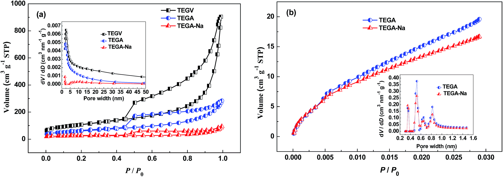 | ||
| Fig. 2 (a) N2 adsorption/desorption isotherms and the corresponding pore size distribution (inset) of TEGV, TEGA and TEGA-Na. (b) CO2 adsorption isotherms and the corresponding pore size distribution (inset) of TEGA and TEGA-Na. | ||
| Sample | SN2a [m2 g−1] | Smicb [m2 g−1] | Sexternalc [m2 g−1] | Smic/SN2d | Vmice [cm3 g−1] | VN2f [cm3 g−1] | Pore sizeg [nm] |
|---|---|---|---|---|---|---|---|
| a SSA calculated with BET method from the N2 adsorption isotherm.b Micropore area based on t-plot method from the N2 adsorption isotherm.c External surface area based on t-plot method from the N2 adsorption isotherm.d Percentage of micropore area based on t-plot method in the BET SSA from the N2 adsorption isotherm.e Micropore volume based on t-plot method from the N2 adsorption isotherm.f Single point adsorption pore volume at P/P0 = 0.97 from the N2 adsorption isotherm.g Adsorption average pore width (4V/A by BET) from the N2 adsorption isotherm. | |||||||
| TEGA | 215 | 20.5 | 194.5 | 9.5% | 0.008 | 0.3675 | 6.8 |
| TEGA-Na | 84 | 57.8 | 26.2 | 68.8% | 0.027 | 0.1069 | 5.09 |
| Sample | SCO2a [m2 g−1] | VCO2b [cm3 g−1] | STotalc [m2 g−1] | VTotald [cm3 g−1] | ρ1e [g cm−3] | ρ2f [g cm−3] |
|---|---|---|---|---|---|---|
| a SSA calculated with DFT method from the CO2 adsorption isotherm.b Pore volume calculated with DFT method from the CO2 adsorption isotherm.c The sum of BET SSA derived from the N2 isotherm and DFT SSA derived from the CO2 isotherm, i.e., STotal = SN2 + SCO2.d The sum of pore volume derived from the N2 isotherm and that from the CO2 isotherm, i.e., VTotal = VN2 + VCO2.e ρ1 is the electrode sheet density, obtained by the compression method based on the total mass of electrode materials, including the graphene material, acetylene black and PTFE.f ρ2 is the apparent density of the graphene sample, calculated by ρ = {VTotal + 1/ρCarbon}−1, where ρCarbon = 2 g cm−3.20 | ||||||
| TEGA | 206.06 | 0.070 | 421.06 | 0.4375 | 0.48 | 1.07 |
| TEGA-Na | 175.42 | 0.057 | 259.42 | 0.1639 | 1.05 | 1.51 |
Similarly, TEGV-K displays the lower total SSA and total pore volume, and hence the higher density compared with TEGV-H and TEGV (Table S3, ESI†). Additionally, a marked feature of TEGV-K different from TEGV-H and TEGV is the presence of the ultramicropores less than 0.4 nm in TEGV-K (Fig. S9c and d, ESI†), probably created by the intercalated K+ ions, as we reported previously.14
The Raman spectra in Fig. S3b (ESI†) indicate that the ID/IG values of all the prepared samples are lower than that of GO, suggesting the recovery of conjugated sp2 graphitic structure. And the recovery degree seems related to the thermal reduction manner: the product obtained by thermal reduction under vacuum, TEGV (0.75), exhibits a higher recovery degree than those thermally reduced in air, TEGA (0.87) and TEGA-Na (0.85). FTIR (Fig. S4a, ESI†) and XPS (Fig. S4b–f, ESI†) spectra of TEGA-Na and TEGA further prove the reduction of GO to a certain degree due to the obvious removal of oxygen-containing groups (Table S1 and S2, ESI†). The C/O ratios determined from the XPS spectra (Fig. S4b, ESI†) of TEGA-Na (5.22) and TEGA (5.78) are very close to each other, indicating their similar content of oxygen-containing groups.
Based on the above analyses, the possible formation mechanism of the thermally expanded graphene assemblies with intercalated cations are tentatively speculated, as illustrated in Scheme 1. The dissociated cations (Na+ or K+) from Na2SO4 or KCl will spontaneously adsorb on GO layers through the electrostatic attraction between positively charged cations and negatively charged oxygen-containing groups on GO layers,21,22 and meanwhile induce the coagulation of GO from its suspension by screening the electrostatic repulsion between adjacent GO layers.19 After desiccation, these cations uniformly reside between the GO layers. Due to the existence of these “pre-intercalated” cations, the coagulated GO aggregates don't stack as firmly as the original graphite oxide. Therefore, when experiencing further thermal treatment, the reduced graphene layers cannot be exfoliated as fiercely as those in graphite oxide (due to lower gas pressure established between better separated layers), consequently forming more uniform and small interlayer pores compared with a thermally expanded product from graphite oxide. Therefore, the as-obtained thermally expanded graphene assemblies with “pre-intercalated” cations exhibit a high apparent density.
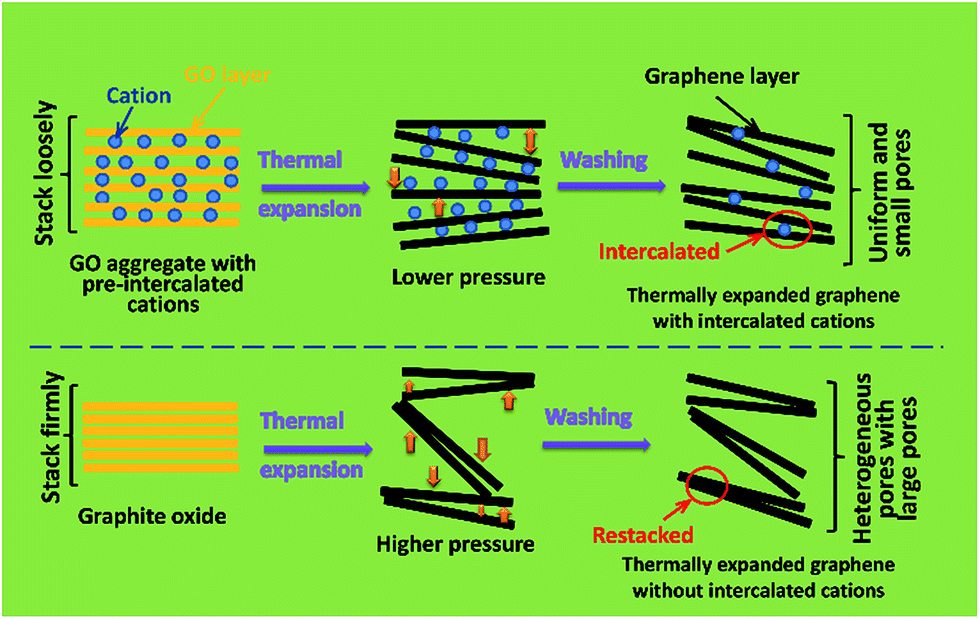 | ||
| Scheme 1 Illustration of the possible formation mechanism of the thermally expanded graphene assemblies with and without pre-intercalated cations. | ||
3.2. Electrochemical performances of the symmetric supercapacitors
The supercapacitive performances of the prepared samples are firstly evaluated using a symmetric two-electrode system in 30 wt% KOH aqueous solution. The CV curves of TEGA-Na in Fig. 3a exhibit a quasi-rectangular shape at scan rates up to 200 mV s−1, indicating the good capacitive characteristics, and the varied capacitance values from the low to high voltage range reveal the existence of pseudo-capacitance provided by faradaic reactions of oxygen-containing groups besides EDL capacitance. Meanwhile, the galvanostatic charge/discharge curves of TEGA-Na (Fig. 3b and c) indicate a good high-rate capability, and the small IR drop at 5 A g−1 (Fig. 3c) discloses an equivalent series resistance (ESR) as low as 9 mΩ g in the case of TEGA-Na. | ||
| Fig. 3 Supercapacitive performances of TEGA-Na and TEGA in a symmetric two-electrode system in 30 wt% KOH aqueous electrolyte. (a) CV curves of TEGA-Na at different scan rates. Galvanostatic charge/discharge curves of TEGA-Na at (b) low and (c) high current densities. (d) Gravimetric capacitances of TEGA-Na and TEGA at different current densities. (e) Cycling stability of the volumetric capacitances of TEGA-Na and TEGA at 1 A g−1. (f) Comparison of gravimetric and volumetric capacitances in aqueous electrolytes of TEGA-Na and TEGA with some representative carbon materials, including RGO-HD,10 KrGO,14 HGF,29 EM-CCG film,13 HPGM12 and activated carbon.30 | ||
Unexpectedly, TEGA-Na exhibits much higher gravimetric capacitance values than TEGA at various current densities (Fig. 3d), even though TEGA-Na has a lower total SSA value (the sum of BET SSA derived from the N2 isotherm and DFT SSA derived from the CO2 isotherm, i.e., the micropores and mesopores are both taken into account) than TEGA, as shown in Table 2. For instance, TEGA-Na and TEGA deliver 217 and 145 F g−1 at 0.1 A g−1, respectively, which correspond to specific areal capacitances of 83 and 34 μF cm−2, calculated on the basis of the total SSA. Taking into account the contribution of pseudo-capacitance, the areal capacitance of 34 μF cm−2 for TEGA is basically reasonable, but the areal capacitance of 83 μF cm−2 for TEGA-Na is much higher than the capacitance of normal carbon (<25 μF cm−2), presumably implying that some small pores have not been identified yet for TEGA-Na through these gas sorption methods. Considering that the bare Na+ ion diameter is only 0.192 nm,23 some pores around or less than 0.4 nm, created by the Na+ ions intercalated in TEGA-Na, might not be detected by the CO2 sorption (lower confidence limit of 0.365 nm) due to the kinetic restrictions,24 or the entrances of some small pores will be opened only after immersing in the electrolyte solution due to the affinity of the Na+ ions intercalated in these pores with the aqueous electrolyte. The latter scenario is quite similar to the “electrochemical activation” of carbons caused by electric field driven intercalation of organic electrolyte ions,25,26 albeit the Na+ ions are “pre-intercalated” herein. Recently, partially desolvated organic electrolyte ions were found to enter carbon pores equal to or smaller than the size of solvated ions, inducing an anomalous increase in capacitance at pore sizes less than 1 nm.27,28 Herein, the probably formed ultramicropores (<0.4 nm) through the intercalation of Na+ ions (no matter opened before or after immersion in aqueous electrolytes) are exactly coincident with such a pore/ion size correlation for aqueous electrolytes, e.g., the effective diameters of alkali cations after hydration were determined to be between 0.362 and 0.42 nm,23 thus partially desolvated or distorted electrolyte ions might penetrate into these ultramicropores, causing the capacitance increase.
The graphene materials prepared under vacuum exhibit exactly the same electrochemical performance regularity: TEGV-K delivers higher gravimetric capacitances at various rates than TEGV (Fig. S10c–e, ESI†), although the total SSA of the former is lower than the latter (Table S3, ESI†), while TEGV-H presents both lower total SSA (Table S3, ESI†) and lower gravimetric capacitances (Fig. S10c–e, ESI†) than TEGV. Because the HCl incorporated in GO aggregates will volatilize during desiccation, the sole difference between TEGV-H and TEGV-K is the pre-intercalation of K+ ions in TEGV-K. Therefore, the ultramicropores (<0.4 nm) (Fig. S9c and d, ESI†) created by the intercalated K+ ions in TEGV-K should be accountable for its anomalously high gravimetric capacitances through the same mechanism as TEGA-Na, as previously reported.14,16
According to the apparent density of TEGA-Na (1.51 g cm−3, Table 2), the volumetric capacitance of TEGA-Na is calculated to be 328 F cm−3 at 0.1 A g−1, about 2.11 times that of TEGA (Fig. S5b, ESI†), and much higher than many porous carbon materials (Fig. 3f). The rate performance curves in Fig. 3d and S5b (ESI†) demonstrate a good high-rate capability of TEGA-Na, while the cycling performance curves in Fig. 3e and S5c (ESI†) confirm an excellent cycling stability of TEGA-Na.
To further enhance the energy density, a symmetric supercapacitor based on TEGA-Na in 1 mol L−1 Na2SO4 aqueous electrolyte was assembled. The CV curves in Fig. 4a show that no obvious distortion of anodic current appears even at a voltage window of 1.8 V. And the CV curves in Fig. 4b and S6a (ESI†) and the galvanostatic charge/discharge curves in Fig. 4c and d display good capacitive characteristics and acceptable rate capability (see also Fig. S6b and S6c, ESI†). The specific capacitance of TEGA-Na is 156 F g−1 (236 F cm−3) at 0.1 A g−1. And the cycling stability has been confirmed with a retention of 81% after 10![[thin space (1/6-em)]](https://www.rsc.org/images/entities/char_2009.gif) 000 cycles (Fig. 4e). The gravimetric Ragone plot of TEGA-Na in Fig. S6d (ESI†) exhibits good energy and power characteristics with an energy density of 17.55 W h kg−1 at 44 W kg−1. As shown in Fig. 4f, the symmetric supercapacitor based on TEGA-Na also exhibits a high volumetric energy density of 26 W h L−1, which is among the highest values for carbon materials reported in aqueous electrolytes.
000 cycles (Fig. 4e). The gravimetric Ragone plot of TEGA-Na in Fig. S6d (ESI†) exhibits good energy and power characteristics with an energy density of 17.55 W h kg−1 at 44 W kg−1. As shown in Fig. 4f, the symmetric supercapacitor based on TEGA-Na also exhibits a high volumetric energy density of 26 W h L−1, which is among the highest values for carbon materials reported in aqueous electrolytes.
 | ||
| Fig. 4 Supercapacitive performances of TEGA-Na in a symmetric two-electrode system in 1 mol L−1 Na2SO4 aqueous electrolyte. (a) CV curves at 50 mV s−1 within different voltage windows. (b) CV curves at high scan rates. Galvanostatic charge/discharge curves at (c) low and (d) high current densities. (e) Cycling retention curve at 5 A g−1. Inset: the CV curves before the 1st cycle and after the 10000th cycle. (f) Comparison of volumetric and gravimetric energy densities in aqueous electrolytes of TEGA-Na with some representative carbon materials, including ALG-C,31 CM,32 FGN-300,9 HPGM,12 FPGM-200,11 KrGO,14 EM-CCG film,13 LN60033 and TTNAG.34 | ||
The supercapacitive performances of TEGA-Na and TEGA are also examined using symmetric supercapacitors in 1 mol L−1 Et4NBF4/AN organic electrolyte. The CV curves in Fig. S7a (ESI†) indicate that higher current density and hence higher gravimetric capacitance are also delivered by TEGA-Na than TEGA in the organic electrolyte. And the cyclic voltammetric results (Fig. S7b–d, ESI†) and galvanostatic charge/discharge results (Fig. S7e and S7f, ESI†) display the reasonable capacitive performances for the microporous material, TEGA-Na.
4. Conclusions
In summary, the high-density graphene assemblies have been prepared via a slightly modified thermal reduction strategy of graphene oxide at mild conditions, which facilitates mass production in large quantities, and manifest their promising application potential in supercapacitors due to their high volumetric performances. Moreover, the effect of cation pre-intercalation on the porosity structure (especially ultramicroporosity) and consequent properties of graphene materials disclosed here might be enlightening, and thus deserves further investigations.Notes and references
- W. Lv, D.-M. Tang, Y.-B. He, C.-H. You, Z.-Q. Shi, X.-C. Chen, C.-M. Chen, P.-X. Hou, C. Liu and Q.-H. Yang, ACS Nano, 2009, 3, 3730–3736 CrossRef CAS PubMed.
- Y. Zhu, S. Murali, M. D. Stoller, A. Velamakanni, R. D. Piner and R. S. Ruoff, Carbon, 2010, 48, 2118–2122 CrossRef CAS.
- H. C. Schniepp, J. L. Li, M. J. McAllister, H. Sai, M. Herrera-Alonso, D. H. Adamson, R. K. Prud'homme, R. Car, D. A. Saville and I. A. Aksay, J. Phys. Chem. B, 2006, 110, 8535–8539 CrossRef CAS PubMed.
- M. F. El-Kady, V. Strong, S. Dubin and R. B. Kaner, Science, 2012, 335, 1326–1330 CrossRef CAS PubMed.
- M.-x. Wang, Q. Liu, H.-f. Sun, E. A. Stach, H. Zhang, L. Stanciu and J. Xie, Carbon, 2012, 50, 3845–3853 CrossRef CAS.
- Y. Wang, Y. Wu, Y. Huang, F. Zhang, X. Yang, Y. Ma and Y. Chen, J. Phys. Chem. C, 2011, 115, 23192–23197 CAS.
- X. Yang, J. Zhu, L. Qiu and D. Li, Adv. Mater., 2011, 23, 2833–2838 CrossRef CAS PubMed.
- Y. Zhu, S. Murali, M. D. Stoller, K. J. Ganesh, W. Cai, P. J. Ferreira, A. Pirkle, R. M. Wallace, K. A. Cychosz, M. Thommes, D. Su, E. A. Stach and R. S. Ruoff, Science, 2011, 332, 1537–1541 CrossRef CAS PubMed.
- J. Yan, Q. Wang, T. Wei, L. Jiang, M. Zhang, X. Jing and Z. Fan, ACS Nano, 2014, 8, 4720–4729 CrossRef CAS PubMed.
- Y. Li and D. Zhao, Chem. Commun., 2015, 51, 5598–5601 RSC.
- L. Jiang, L. Sheng, C. Long, T. Wei and Z. Fan, Adv. Energy Mater., 2015, 5, 1500771 Search PubMed.
- Y. Tao, X. Xie, W. Lv, D.-M. Tang, D. Kong, Z. Huang, H. Nishihara, T. Ishii, B. Li, D. Golberg, F. Kang, T. Kyotani and Q.-H. Yang, Sci. Rep., 2013, 3, 2975 Search PubMed.
- X. Yang, C. Cheng, Y. Wang, L. Qiu and D. Li, Science, 2013, 341, 534–537 CrossRef CAS PubMed.
- D. Q. Liu, Z. Jia, J. X. Zhu and D. L. Wang, J. Mater. Chem. A, 2015, 3, 12653–12662 CAS.
- J. Zhou, J. Lian, L. Hou, J. Zhang, H. Gou, M. Xia, Y. Zhao, T. A. Strobel, L. Tao and F. Gao, Nat. Commun., 2015, 6, 8503 CrossRef CAS PubMed.
- X. Wu, J. Zhou, W. Xing, Y. Zhang, P. Bai, B. Xu, S. Zhuo, Q. Xue and Z. Yan, Carbon, 2015, 94, 560–567 CrossRef CAS.
- D. Q. Liu, Z. Jia and D. L. Wang, Carbon, 2016, 100, 664–677 CrossRef CAS.
- Z. Jia, C. Li, D. Liu and L. Jiang, RSC Adv., 2015, 5, 81030–81037 RSC.
- J. P. Rong, M. Y. Ge, X. Fang and C. W. Zhou, Nano Lett., 2014, 14, 473–479 CrossRef CAS PubMed.
- H. Nishihara and T. Kyotani, Adv. Mater., 2012, 24, 4473–4498 CrossRef CAS PubMed.
- S. Park, K.-S. Lee, G. Bozoklu, W. Cai, S. T. Nguyen and R. S. Ruoff, ACS Nano, 2008, 2, 572–578 CrossRef CAS PubMed.
- S. Salgado, L. Pu and V. Maheshwari, J. Phys. Chem. C, 2012, 116, 12124–12130 CAS.
- L. Eliad, G. Salitra, A. Soffer and D. Aurbach, J. Phys. Chem. B, 2001, 105, 6880–6887 CrossRef CAS.
- R. V. R. A. Rios, J. Silvertre-Albero, A. Sepulveda-Escribano, M. Molina-Sabio and F. Rodriguez-Reinoso, J. Phys. Chem. C, 2007, 111, 3803–3805 CAS.
- B. H. Ka and S. M. Oh, J. Electrochem. Soc., 2008, 155, A685–A692 CrossRef CAS.
- M. M. Hantel, T. Kaspar, R. Nesper, A. Wokaun and R. Kotz, Electrochem. Commun., 2011, 13, 90–92 CrossRef CAS.
- J. Chmiola, G. Yushin, Y. Gogotsi, C. Portet, P. Simon and P. L. Taberna, Science, 2006, 313, 1760–1763 CrossRef CAS PubMed.
- J. Chmiola, C. Largeot, P. L. Taberna, P. Simon and Y. Gogotsi, Angew. Chem., Int. Ed., 2008, 47, 3392–3395 CrossRef CAS PubMed.
- Y. Xu, Z. Lin, X. Zhong, X. Huang, N. O. Weiss, Y. Huang and X. Duan, Nat. Commun., 2014, 5, 4554 CAS.
- B. Xu, Y. Chen, G. Wei, G. Cao, H. Zhang and Y. Yang, Mater. Chem. Phys., 2010, 124, 504–509 CrossRef CAS.
- E. Raymundo-Pinero, F. Leroux and F. Beguin, Adv. Mater., 2006, 18, 1877–1882 CrossRef CAS.
- M. Kunowsky, A. Garcia-Gomez, V. Barranco, J. M. Rojo, J. Ibanez, J. D. Carruthers and A. Linares-Solano, Carbon, 2014, 68, 553–562 CrossRef CAS.
- E. Raymundo-Pinero, M. Cadek and F. Beguin, Adv. Funct. Mater., 2009, 19, 1032–1039 CrossRef CAS.
- N. Xiao, H. Tan, J. Zhu, L. Tan, X. Rui, X. Dong and Q. Yan, ACS Appl. Mater. Interfaces, 2013, 5, 9656–9662 CAS.
Footnote |
| † Electronic supplementary information (ESI) available: Preparation of graphite oxide, characterization and supercapacitive performances of the samples. See DOI: 10.1039/c6ra03897b |
| This journal is © The Royal Society of Chemistry 2016 |