Electronic and optical properties of surface hydrogenated armchair graphene nanoribbons: a theoretical study

Abstract

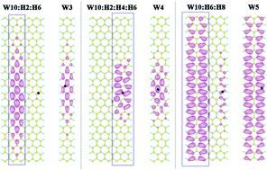
The electronic and optical properties of surface hydrogenated armchair graphene nanoribbons (H-AGNRs) are investigated by first-principle ab initio calculations with quasi-particle corrections. The variation in band gaps is scrutinized in terms of bonding characteristics and the localization of wavefunctions. Optical absorption spectra, exciton binding energies and exciton wavefunctions are investigated with the consideration of different hydrogen adsorption row positions and coverages. Instead of the traditional family effect in pristine AGNRs, we introduce an effective width model to provide a more general understanding for H-AGNRs. The calculations show that the effective width segment in H-AGNRs plays an important role in the band gaps and excitons. Moreover, the spatial distributions of the electronic and exciton wavefunctions are confined by hydrogen atoms, revealing a self-confinement pseudo quantum well.

---

Introduction

Graphene, a single layer of graphite, has been developed at a fantastic pace,^1–7 after the successful syntheses in experiments.^8–13 Graphene is important for both fundamental condensed matter physics, including quantum hall effects,¹⁰ spin qubits,¹⁴ photochemistry¹⁵ and pH sensors,¹⁶ and for its promising application in emerging areas, such as electronic devices,^17–21 spintronic devices^22–25 and hydrogen storage materials.^26–28 The surface chemistry can be crucial in real reactions; it was reported that the surface is sensitive to small molecules and the transport performance is influenced dramatically after hydrogen adsorption.^29–34 A graphene surface is also sensitive, and it can have covalent^35–38 or non-covalent³⁹ functionalization by chemicals. Hydrogen is one of the most basic chemical groups for graphene surface functionalization, and moreover the properties of graphene, such as the metallic state, lattice spacing and even the quantum hall effect, can be controlled by the hydrogenation in several ways.^27,28,40 For example, hydrogenation on graphene can be experimentally reversible and restored by thermal annealing.^27,28,40 Hydrogen also plays a significant role in the preparation of graphene on a copper surface⁴¹ and in the design of graphene-based materials for high-power electrodes.⁴² A polyhydrogenated graphene, obtained from a Birch-type reduction of graphite, possesses a very strong fluorescence, revealing its potential for optoelectronics.⁴³

Not only can the surface of graphene be chemically modified, the edges can also be controlled through functionalization. Through chemical etching, nanosize quasi one-dimensional graphene nanoribbons (GNRs) with different edges can be obtained^44,45 which led to remarkable work on the study of the variant properties of GNRs.⁴⁶ GNRs with armchair edges (AGNRs) have direct band gaps and moreover there is a distinct family effect, which defines W(n) for AGNRs and classifies AGNRs into three families: n = 3p, 3p + 1 and 3p + 2, where p is a positive integer and n is the width index.^47,48 Previous studies^49,50 also describe the scaling character of the exciton behavior in pristine AGNRs and the electron and exciton wavefunctions in armchair graphene nanoribbons passivated by hydrogen and/or fluorine atoms. In this work we perform a comprehensive study on the electronic and optical properties of hydrogenated AGNRs (H-AGNRs) through variant adsorption row positions and the hydrogen coverage on the surface and also introduce an effective width model for the H-AGNRs, providing an effective way to control the optoelectronic applications.

Theoretical methods and models

The first-principles calculation of the optical excitations is carried out using a many-body perturbation theory approach, based on the several procedure.⁵¹ First we calculate the ground state wavefunction of the fully relaxed structures using the local density approximation (LDA) using the Quantum-ESPRESSO code.⁵² Separable norm-conserving pseudo potentials and a plane-wave basis set are used for the calculations. A kinetic energy cutoff of 60 Ry and 71 × 1 × 1 k-samplings are applied along the periodical x-direction, and a minimal 20 Å distance is kept for the other two non-periodic directions. Each atomic structure is fully relaxed with the forces per atoms converged to 0.01 eV Å⁻¹. The quasi-particle corrections to eigenvalues under the LDA scheme are computed within the G0W0 approximation for the self-energy operator, and the electronic screening is treated by the plasmon-pole approximation.⁵³ The electron–hole interaction is included by solving the Bethe–Salpeter equation (BSE) in the basis set of quasi-electron and quasi-hole states, where the static screening in the direct term is calculated within the random-phase approximation:⁵⁴
where A^S_vck represents the exciton wavefunction, K^eh is the electron–hole coupling kernel, Ω^S is the energy of the given excitation, and E_ck and E_vk are the quasi-particle energies of the electron and hole states, respectively. 20 valence bands and 20 conduction bands are considered for the GW calculations. 10 valence bands and 10 conduction bands are considered in the BSE calculation. All the G0W0-BSE calculations are performed with the Yambo code⁵⁵ for light polarized along the ribbon principal axis, i.e. the x-axis, as shown in Fig. 1. A supercell is applied to mimic the quasi one-dimensional GNR structures in our calculations, and a rectangular-shape truncated Coulomb interaction is applied to eliminate the image effect between adjacent supercells to mimic isolated GNRs.⁵⁶

Fig. 1 (Top) Atomic structures of W8, W9, and W10 H-AGNRs, and the numbers on the left label the row position. The red dots denote the positions for hydrogen adsorption. (Bottom) Schematic structure of W8:H4 in the top- and side-views.

The atomic structures of the W(n) AGNRs are shown in Fig. 1, where n is the width index of the AGNR. Three typical atomic structures of W8, W9, and W10 AGNRs are investigated. Since there are a lot of hydrogenated graphene structures based on different adsorption positions, we only select several structures to investigate. The hydrogen atoms adsorb on rows of the AGNRs, marked by red dots in the top of Fig. 1. To minimize the asymmetry strain energy, two hydrogen atoms of the same row adsorb on both sides of the AGNRs.⁴⁰ The hydrogen coverage ratio is decided by the numbers of adsorbed hydrogen rows. In this work, we mainly focus on the low coverage cases. We also define the hydrogenated AGNRs (H-AGNRs) as W(m):H(n):H(k):H(l), where m is the width index of the ANGRs, and n, k, and l are denoted as the indexes of the hydrogen rows. W8:H4 is schematically shown in the bottom of Fig. 1 as an example.

Since there are different rows for the adsorption of hydrogen atoms, most H-AGNRs have two or more configurations. For example, in one-row H-AGNRs, there is W8:H2, W8:H4, W8:H6, W9:H3, W9:H5, W10:H2, W10:H4, W10:H6 and W10:H8 for hydrogenated W8, W9 and W10 AGNRs, respectively. Additionally, in the multi-row H-AGNRs, due to the up and down duality between two hydrogen rows, there are two or more configurations. For example, in the W8:H2:H6 structure, there are two configurations for hydrogen adsorption. However, we find that the differences of the electronic and optical characteristics between these two structures are very tiny (S1, ESI†), therefore we only consider one of them with the name W8:H2:H6 and in the other multi-row cases as well.

Results and discussion

The analyses of hydrogenation and the effective width model

The adsorption of hydrogen atoms process turns sp² hybridization of carbon to sp³ hybridization, possessing a little deviation of the plane due to the sp³ carbon atom, with an increase of the bond length from 1.42 Å to 1.49 Å, and around a 30 degree torsion (see W8:H4 in Fig. 1).^49,50 Due to the formation of the C–H bonds, the energy of the p_z orbital in the sp³ carbon will shift into the lower energy side,^49,50 beyond the energy range of canonical π-bonding.

Tables 1–3 summarize the LDA band gaps, GW band gaps, BSE energies and the binding energies for the one-, two- and three-row W8, W9, and W10 H-ANGRs. It is noticed that W(m):H(n) structures in the same W(m) series have different band gaps. For example, W9:H5 has a larger band gap than that of W9:H3 (Table 1). At first glance, it is difficult to find a similar family behaviour in W(m):H(n). To understand the possible internal trend, the nature of the pristine AGNRs is considered first. The pristine AGNRs only have sp² networks, while the hydrogenation in the H-AGNRs turns sp² to sp³ hybridization, which lets us logically introduce an effective width model of the sp² network to estimate the trend of the H-AGNRs. In the W(m):H(n) structure, it is divided into two parts by the hydrogen atoms, which are indicated as W(n − 1) and W(m − n − 1) with the segment widths of (n − 1) and (m − n − 1). In W9:H3, there are two divided parts, W2 and W6, which belong to the 3p + 2 and 3p families, respectively. The LDA band gap of W2 (1.18 eV) is larger than that of W6 (0.99 eV).⁴⁹ W9:H3 has a 0.98 eV LDA band gap (Table 1), which is close to W6. In W9:H5, there are two W4 parts, which belong to the 3p + 1 family. The LDA band gap of W4 is 2.53 eV,⁴⁹ while that of W9:H5 is 2.15 eV. Consequently, it reveals that the band gap of W(m):H(n) is close to the smaller band gap of the segment, which can be considered as an effective width segment in the effective width model. Since W6 is the effective width segment in W9:H3, it is shortened as EW-W6 for W9:H3. Herein, it is easy to find out that W9:H5 has a larger band gap than that of W9:H3 through the comparison of EW-W4 and EW-W6 via the effective width model. A similar trend also exists in the W8:H(n) and W10:H(n) structures (S2, ESI†). Correspondingly, the smallest band gap part can be considered as a quantum well in K space which affects the valence band maximum (VBM) and conduction band minimum (CBM).

Table 1 Summary of LDA band gaps, GW band gaps, BSE energies and binding energies for the one-row W8, W9, and W10 H-ANGRs

W	LDA (eV)	GW (eV)	BSE (eV)	Eb (eV)
W8	0.26	1.09	0.29	0.80
W8:H2	0.95	2.79	1.32	1.47
W8:H4	1.59	4.21	2.88	1.33
W8:H6	0.41	1.71	0.69	1.02
W9	0.69	2.12	0.92	1.20
W9:H3	0.98	2.84	1.36	1.48
W9:H5	2.15	4.89	3.06	1.83
W10	1.24	3.12	1.57	1.41
W10:H2	0.35	1.39	0.47	0.92
W10:H4	0.89	2.67	1.33	1.34
W10:H6	0.52	1.94	0.74	1.20
W10:H8	1.02	3.11	1.58	1.53

---

In the W(m):H(n):H(k) and W(m):H(n):H(k):H(l) structures, which have two and three hydrogen adsorption rows, the trend of the band gaps (Tables 2 and 3) can be studied in a similar way based on the effective width model (S2, ESI†). The effective width segment is the one having the smallest band gap.

Table 2 Summary of LDA band gaps, GW band gaps, BSE energies and binding energies for the two-row W8, W9 and W10 H-ANGRs

W	LDA (eV)	GW (eV)	BSE (eV)	Eb (eV)
W8:H2:H4	2.28	5.30	3.15	2.15
W8:H2:H6	1.12	3.49	1.74	1.75
W8:H4:H6	1.02	3.41	1.68	1.73
W9:H3:H5	1.02	3.38	1.70	1.68
W9:H3:H7	1.08	3.36	1.73	1.63
W10:H2:H4	0.98	2.83	1.41	1.42
W10:H2:H6	1.36	3.74	2.06	1.68
W10:H2:H8	0.45	1.78	0.75	1.03
W10:H4:H6	1.68	4.35	2.95	1.40
W10:H4:H8	1.12	3.39	1.73	1.66
W10:H6:H8	0.48	1.80	0.71	1.09

---

Table 3 Summary of LDA band gaps, GW band gaps, BSE energies and binding energies for the three-row W8, W9, and W10 H-ANGRs

W	LDA (eV)	GW (eV)	BSE (eV)	Eb (eV)
W8:H2:H4:H6	1.02	3.49	1.72	1.77
W9:H3:H5:H7	0.96	3.34	1.70	1.64
W10:H2:H4:H6	2.22	5.35	3.35	2.00
W10:H2:H4:H8	1.10	3.41	1.74	1.67
W10:H2:H6:H8	1.02	3.35	1.70	1.65
W10:H4:H6:H8	1.02	3.38	1.68	1.70

---

The analyses of GW corrections and exciton wavefunctions

The quasi-particle GW band gaps have energy corrections of the LDA band gaps in the order of 1 eV (Tables 1–3) and are greater than those in bulk graphite or diamond due to the ineffective screening for reduced dimensions.⁵⁷ The optical transition energies are computed by solving the BSE numerically. Only the first optical transition energies associated with bound excitons are listed in the fourth column (Tables 1–3). Firstly, most of the oscillator strength is transferred from the inter-band to the exciton transitions, which dominate the optical absorption spectra. Secondly, the order of optical energies correlates with the energy gaps for all the cases accordingly. The absolute values of optical energies are about half of the GW gap values which are the clear manifestation of strong coupling of the electron and hole in the H-AGNRs.

The exciton binding energy (E_b) is defined as the difference between the GW band gap and the optical transition energy. The binding energies range from 1.00 to 2.15 eV for the hydrogen adsorption cases (Tables 1–3). In general, the electron–hole interaction kernel has an attractive direct term by the screened Coulomb interaction and a repulsive exchange term mediated by the bare Coulomb interaction.²³ For example, the GW gap of W10:H8 is 3.11 eV, which results in a significantly heavier effective mass (larger kinetic energy)²⁹ and a reasonably weaker screening to reduce the Coulomb interaction between the electron and hole. Therefore, its exciton binding energy is the strongest in the W10:H(n) series. Similarly, the exciton binding energy of W9:H5 is the strongest in the W9:H(n) series due to the heavier effective mass and weaker screening.

Next we further gain insight into the effects of electron–hole interaction by showing the exciton wavefunctions with the lowest excitation energy in real space with one fixed hole position for all the functionalized AGNRs studied in this work. For the H-AGNRs with different adsorption rows, the general patterns of exciton wavefunctions are very different. For the one-row cases, as shown in Fig. 2(a)–(c), most exciton wavefunctions locate near one edge, and their spatial distribution can be understood by performing the direct product of wavefunctions of the VBM and CBM at the Γ point as shown in Fig. S3 (ESI†). Fig. 2(d) and (e) show the sizes of the wavefunction projected along the x-axis direction. In Fig. 2(d), it is noticed that all one-row W8 H-AGNRs have smaller wavefunction sizes than the pristine W8 AGNR due to the increase of the exciton binding energy. The W9 serials in Fig. 2(e) also show a similar phenomenon. Additionally, due to the lowest binding energy of W10:H2, it has the largest sized exciton wavefunction among the W10 H-AGNRs and the W10 AGNR (Fig. 2(f)).

Fig. 2 Exciton wavefunctions of one-row (a) W8, (b) W9, and (c) W10 H-AGNRs. The isovalue is 0.01. (d)–(f) Exciton wavefunctions projected along the x-axis for W8, W9, and W10 serials, respectively. Only the outlines are shown for clarity.

The exciton wavefunctions of the two-row H-AGNRs are shown in Fig. 3(a)–(c) and their exciton sizes along the x-axis direction are plotted in Fig. 3(e)–(f), similar to the one-row cases. Most of the spatial distribution of the exciton wavefunction is dependent on the distribution of the VBM and CBM (Fig. S4, ESI†), except for W9:H3:H7. Although the VBM and CBM of W9:H3:H7 distribute symmetrically on both edges (Fig. S4, ESI†), since the hole position locates on one edge, the exciton wavefunction only lies on the same edge. Most two-row H-AGNRs have smaller exciton sizes due to the larger band gaps than those of the respective pristine AGNRs, however, W10:H2:H8 still has a larger exciton size than the pristine W10 AGNR (Fig. 3(f)).

Fig. 3 Exciton wavefunctions of two-row (a) W8, (b) W9, and (c) W10 H-AGNRs. The isovalue is 0.01. (d)–(f) Exciton wavefunctions projected along the x-axis for W8, W9, and W10 serials, respectively. Only the outlines are shown for clarity.

When the coverage of the surface hydrogen is increased, the AGNR is divided into much smaller fragments. According to previous work,^47–50 the band gaps increase with the decrease of widths in the same family of pristine AGNRs. Consequently, the high coverage of the hydrogen cuts the pristine AGNR into small pieces in the H-AGNR, and increases the band gap and exciton binding energy as well. In the three-row H-AGNRs (Fig. 4(a)–(f)), there is an obvious shrink of the exciton wavefunction both in the spatial distribution and the size, in comparison to the one- and two-row H-AGNRs. Different from the fully hydrogenated graphene structure (graphene),⁵⁸ in most two- and three-row adsorption cases, we also notice that both the VBM/CBM (in Fig. S4 and S5, ESI†) and the exciton wavefunction spatial distributions (Fig. 3 and 4) are confined in one block region separated by the hydrogen atoms, indicating the confinement effect, which is related with the hydrogen coverage and adsorption row position; that is, the electronic and optical properties of these cases are affected by this confinement effect.

Fig. 4 Exciton wavefunctions of three-row (a) W8, (b) W9, and (c) W10 H-AGNRs. The isovalue is 0.01. (d)–(f) Exciton wavefunctions projected along the x-axis for W8, W9, and W10 serials, respectively. Only the outlines are shown for clarity.

The analysis of H-AGNRs within the same effective width segments

There are several H-AGNRs with equivalent effective width segments (EW-W3, EW-W4 and EW-W5) which are divided by hydrogen rows, so it is necessary to investigate the differences between EW-W3, EW-W4 and EW-W5 in the H-AGNRs. Herein we only consider several H-AGNRs whose band gaps and the exciton wavefunctions are dominated by the corresponding EW-W3, EW-W4, and EW-W5. We summarize their LDA band gaps, GW band gaps, BSE energies and the binding energies in Table 4. Compared with pristine W3, W4, and W5 AGNRs, the band gaps and the binding energies are smaller in the H-AGNRs within the same equivalent ones, and the extent of the confinement is dominate for the tiny difference as well. To deeply understand the tiny difference between the cases which possess the same effective width segments, we first consider W8:H6 and W10:H6 as examples, both of which have EW-W5. We know that the hydrogen rows divide W8:H6 into W5 and W2 segments, and separate W5 and W4 segments in W10:H6. In Table 4, it is found that W8:H6 has a smaller band gap than that of W10:H6, which may be relevant to the fact that the band gap of W2 is smaller than that of W4. Additionally, the band gap can be affected by other factors as well. Take W10:H2:H6 and W10:H4:H6 as examples. Both cases possess EW-W3 and also have the same hydrogen row. It is found that in W10:H2:H6, W3 is confined by sp³ bonds on both sides, while in W10:H4:H6, W3 is confined by sp³ bonds on one side and sp² bonds on the other side, thus the latter one is half confined (Fig. 3(c)), which is close to the pristine W3 AGNR. Moreover, the band gap, BSE energy and the binding energy of W10:H4:H6 is much closer to the original W3 rather than W10:H2:H6 and other structures having EW-W3 (Table 4). As a consideration of W10:H2:H8 and W10:H6:H8, both H-AGNRs contain EW-W5, and have similar band gaps, BSE energies and binding energies (Table 4). Although W10:H6:H8 is half confined compared to W10:H2:H8 (Fig. 3(c)), the band gap of H-AGNRs is mainly influenced by the smallest band gap segment. Since EW-W5 belongs to the 3p + 2 family and has the smallest band gap in comparison to the 3p and 3p + 1 families of other segments, EW-W5 dominates with a majority and dilutes other effects for the confinement, and consequently W10:H6:H8 shows similar characteristics to W10:H2:H8.

Table 4 Summary of LDA band gaps, GW band gaps, BSE energies and binding energies for (H-)AGNRs with (EW-)W3, W4 and W5

W		LDA (eV)	GW (eV)	BSE (eV)	Eb (eV)
W3		1.7	4.69	2.43	2.26
EW-W3	W8:H4	1.59	4.21	2.88	1.33
	W10:H2:H6	1.36	3.74	2.06	1.68
	W10:H4:H6	1.68	4.35	2.95	1.4
W4		2.53	5.41	2.66	2.75
EW-W4	W8:H2:H4	2.28	5.3	3.15	2.15
	W10:H2:H4:H6	2.22	5.35	3.35	2
W5		0.56	2.07	0.75	1.32
EW-W5	W8:H6	0.41	1.71	0.69	1.02
	W10:H6	0.52	1.94	0.74	1.2
	W10:H2:H8	0.45	1.78	0.75	1.03
	W10:H6:H8	0.48	1.8	0.71	1.09

---

The comparison between the effective width model and pristine AGNRs

To clarify the effective width effects, we also investigate the exciton wavefunctions of three W10 H-AGNRs possessing EW-W3, EW-W4 and EW-W5, and compare them with pristine W10, W3, W4 and W5 AGNRs, as shown in Fig. 5. Each pair is separated by a black dashed line in Fig. 5 and the confinement areas are marked by the blue rectangles as well. As discussed above, W10:H2:H6 has EW-W3, confined by sp³ boundaries on both sides, which are soft walls and allow the VBM and CBM wavefunction to leak across the walls (Fig. S6, ESI†), in comparison to the sp² boundaries on both sides of the pristine AGNRs, which have hard walls and no wavefunction leakage. Compared with the hard confinement conditions in the pristine AGNRs, the soft confinement wall relatively decreases the band gap in the respective H-AGNRs. Thus, W10:H2:H6 with a confined EW-W3 has a smaller band gap than the pristine W3, resulting in a smaller effective mass and a larger static dielectric constant,^49,50 and finally the exciton binding energy decreases as well. Similar phenomena also exist in other H-AGNRs possessing the effective width segments of W4 and W5 (Fig. 5), revealing that the confinement is very important for the exciton characteristics, the exciton binding energies and the spatial distributions of the wavefunctions. The positions of the adsorption hydrogen atoms form a self-confinement pseudo quantum well in most H-AGNRs. Furthermore, the confinement can be understood by the effective width model as we discussed above.

Fig. 5 Exciton wavefunctions for W10, W10:H2:H6, W3, W10:H2:H4:H6, W4, W10:H6:H8 and W5, respectively. The isovalue is 0.05 for all the cases. The black dashed lines separate the (H-)AGNRs dependent on the (effective) width and the blue rectangles indicate the superlattice areas of quantum well confinement in the H-AGNRs.

It is noted that some experimental works reported quantum well structures in a graphene superlattice,^59,60 which was built from graphene nanoribbons with a different width. Previous work⁶¹ also reported a hydrocarbon lithography method to create artificial patterns in a graphene surface, which is very close to our model. Moreover, previous work^62–64 also mentioned that with a suitable choice of the precursor, a wide range of materials can be deposited on graphene by an electron-beam to create nanometer-scale doping patterns or etch masks, which is also feasible for our structure. Our present investigations call for experiments addressing the optical features of H-AGNRs including the quantum well effect. A combined theoretical and experimental understanding of hydrogenation as a control parameter for the performance can be considered as an important step toward the future design and application of graphene optoelectronics.

Conclusions

We perform first-principle ab initio calculations on H-AGNRs with quasi-particle corrections and discuss the configurations with variant hydrogen row position and hydrogen coverage, which determine the electronic and optical properties. We introduce a directly and systematically effective width model to understand the band gap variation and the spatial distribution of the VBM/CBM and exciton wavefunctions, providing an effective way to control the optoelectronic applications. Additionally, the positions of adsorption hydrogen atoms form a self-confinement pseudo quantum well in most H-AGNRs, giving potential quantum well applications.

Acknowledgements

This work was financially supported by the National Natural Science Foundation of China (Grant No. 21203154, 51503172 and 81571807) and Fundamental Research Funds for the Central Universities (Grant No. XDJK2016B001). Computation resource is supported by Faculty of Materials and Energy of Southwest University.

Notes and references

1. A. K. Geim and K. S. Novoselov, Nat. Mater., 2007, 6, 183–191.
2. A. K. Geim, Science, 2009, 324, 1530–1534.
3. X. An and J. C. Yu, RSC Adv., 2011, 1, 1426–1434.
4. S. Bai and X. Shen, RSC Adv., 2012, 2, 64–98.
5. B. Liu, F. Meng, C. D. Reddy, J. A. Baimova, N. Srikanth, S. V. Dmitriev and K. Zhou, RSC Adv., 2015, 5, 29193–29200.
6. M. Wang, Y. C. Wang, H. X. Zhao and S. X. Song, RSC Adv., 2015, 5, 68722–68727.
7. W. X. Zhang, C. He, T. Li and S. B. Gong, RSC Adv., 2015, 5, 33407–33413.
8. K. S. Novoselov, A. K. Geim, S. V. Morozov, D. Jiang, Y. Zhang, S. V. Dubonos, I. V. Grigorieva and A. A. Firsov, Science, 2004, 306, 666–669.
9. K. S. Novoselov, A. K. Geim, S. V. Morozov, D. Jiang, M. I. Katsnelson, I. V. Grigorieva, S. V. Dubonos and A. A. Firsov, Nature, 2005, 438, 197–200.
10. Y. B. Zhang, Y. W. Tan, H. L. Stormer and P. Kim, Nature, 2005, 438, 201–204.
11. M. Wang, S. X. Song, H. X. Zhao, Y. C. Wang, L. Y. Zhang and D. Y. Liu, Mater. Lett., 2016, 163, 187–191.
12. H.-X. Zhao, Y.-C. Wang, L.-Y. Zhang and M. Wang, New J. Chem., 2015, 39, 98–101.
13. X. Zhu and H. Su, ACS Nano, 2014, 8, 1284–1289.
14. B. Trauzettel, D. V. Bulaev, D. Loss and G. Burkard, Nat. Phys., 2007, 3, 192–196.
15. H. T. Liu, S. M. Ryu, Z. Y. Chen, M. L. Steigerwald, C. Nuckolls and L. E. Brus, J. Am. Chem. Soc., 2009, 131, 17099.
16. P. K. Ang, W. Chen, A. T. S. Wee and K. P. Loh, J. Am. Chem. Soc., 2008, 130, 14392.
17. P. Blake, P. D. Brimicombe, R. R. Nair, T. J. Booth, D. Jiang, F. Schedin, L. A. Ponomarenko, S. V. Morozov, H. F. Gleeson, E. W. Hill, A. K. Geim and K. S. Novoselov, Nano Lett., 2008, 8, 1704–1708.
18. D. Gunlycke, D. A. Areshkin, J. W. Li, J. W. Mintmire and C. T. White, Nano Lett., 2007, 7, 3608–3611.
19. S. Gilje, S. Han, M. Wang, K. L. Wang and R. B. Kaner, Nano Lett., 2007, 7, 3394–3398.
20. M. C. Lemme, T. J. Echtermeyer, M. Baus and H. Kurz, IEEE Electron Device Lett., 2007, 28, 282–284.
21. M. Q. Long, L. Tang, D. Wang, L. J. Wang and Z. G. Shuai, J. Am. Chem. Soc., 2009, 131, 17728–17729.
22. N. Tombros, C. Jozsa, M. Popinciuc, H. T. Jonkman and B. J. van Wees, Nature, 2007, 448, 571–U574.
23. O. V. Yazyev and M. I. Katsnelson, Phys. Rev. Lett., 2008, 100, 047209.
24. M. Ezawa, New J. Phys., 2009, 11, 095005.
25. Y. W. Son, M. L. Cohen and S. G. Louie, Nature, 2006, 444, 347–349.
26. J. O. Sofo, A. S. Chaudhari and G. D. Barber, Phys. Rev. B: Condens. Matter Mater. Phys., 2007, 75, 153401.
27. R. Balog, B. Jorgensen, J. Wells, E. Laegsgaard, P. Hofmann, F. Besenbacher and L. Hornekaer, J. Am. Chem. Soc., 2009, 131, 8744.
28. L. Hornekaer, E. Rauls, W. Xu, Z. Sljivancanin, R. Otero, I. Stensgaard, E. Laegsgaard, B. Hammer and F. Besenbacher, Phys. Rev. Lett., 2006, 97, 186102.
29. J. Kong, N. R. Franklin, C. W. Zhou, M. G. Chapline, S. Peng, K. J. Cho and H. J. Dai, Science, 2000, 287, 622–625.
30. P. G. Collins, K. Bradley, M. Ishigami and A. Zettl, Science, 2000, 287, 1801–1804.
31. X. Zhu, G. A. Chass, L.-C. Kwek, A. L. Rogach and H. Su, J. Phys. Chem. C, 2015, 119, 29171–29177.
32. Q. Zhao, X. Zhu, X. Bai, H. Fan and Y. Xie, Eur. J. Inorg. Chem., 2007, 2007, 1829–1834.
33. Z.-C. Wu, X. Zhu, C. Pan, Z.-Y. Yao and Y. Xie, Chin. J. Inorg. Chem., 2006, 22, 1371–1374.
34. S. Amini, A. Masic, L. Bertinetti, J. S. Teguh, J. S. Herrin, X. Zhu, H. Su and A. Miserez, Nat. Commun., 2014, 5, 3187.
35. I. Gierz, C. Riedl, U. Starke, C. R. Ast and K. Kern, Nano Lett., 2008, 8, 4603–4607.
36. T. Ohta, A. Bostwick, T. Seyller, K. Horn and E. Rotenberg, Science, 2006, 313, 951–954.
37. S. Y. Zhou, D. A. Siegel, A. V. Fedorov and A. Lanzara, Phys. Rev. Lett., 2008, 101, 086402.
38. W. Chen, S. Chen, D. C. Qi, X. Y. Gao and A. T. S. Wee, J. Am. Chem. Soc., 2007, 129, 10418–10422.
39. Y. X. Xu, H. Bai, G. W. Lu, C. Li and G. Q. Shi, J. Am. Chem. Soc., 2008, 130, 5856.
40. D. C. Elias, R. R. Nair, T. M. G. Mohiuddin, S. V. Morozov, P. Blake, M. P. Halsall, A. C. Ferrari, D. W. Boukhvalov, M. I. Katsnelson, A. K. Geim and K. S. Novoselov, Science, 2009, 323, 610–613.
41. X. Zhang, L. Wang, J. Xin, B. I. Yakobson and F. Ding, J. Am. Chem. Soc., 2014, 136, 3040–3047.
42. J. Ye, M. T. Ong, T. W. Heo, P. G. Campbell, M. A. Worsley, Y. Liu, S. J. Shin, S. Charnvanichborikarn, M. J. Matthews, M. Bagge-Hansen, J. R. I. Lee, B. C. Wood and Y. M. Wang, Sci. Rep., 2015, 5, 16190.
43. R. A. Schafer, J. M. Englert, P. Wehrfritz, W. Bauer, F. Hauke, T. Seyller and A. Hirsch, Angew. Chem., Int. Ed., 2013, 52, 754–757.
44. M. Y. Han, B. Ozyilmaz, Y. B. Zhang and P. Kim, Phys. Rev. Lett., 2007, 98, 206805.
45. Z. H. Chen, Y. M. Lin, M. J. Rooks and P. Avouris, Phys. E, 2007, 40, 228–232.
46. A. H. Castro Neto, F. Guinea, N. M. R. Peres, K. S. Novoselov and A. K. Geim, Rev. Mod. Phys., 2009, 81, 109.
47. Y. W. Son, M. L. Cohen and S. G. Louie, Phys. Rev. Lett., 2006, 97, 216803.
48. L. Yang, C.-H. Park, Y.-W. Son, M. L. Cohen and S. G. Louie, Phys. Rev. Lett., 2007, 99, 186801.
49. X. Zhu and H. Su, J. Phys. Chem. A, 2011, 115, 11998–12003.
50. X. Zhu and H. Su, J. Phys. Chem. C, 2010, 114, 17257–17262.
51. G. Onida, L. Reining and A. Rubio, Rev. Mod. Phys., 2002, 74, 601.
52. P. Giannozzi, S. Baroni, N. Bonini, M. Calandra, R. Car, C. Cavazzoni, D. Ceresoli, G. L. Chiarotti, M. Cococcioni, I. Dabo, A. Dal Corso, S. de Gironcoli, S. Fabris, G. Fratesi, R. Gebauer, U. Gerstmann, C. Gougoussis, A. Kokalj, M. Lazzeri, L. Martin-Samos, N. Marzari, F. Mauri, R. Mazzarello, S. Paolini, A. Pasquarello, L. Paulatto, C. Sbraccia, S. Scandolo, G. Sclauzero, A. P. Seitsonen, A. Smogunov, P. Umari and R. M. Wentzcovitch, J. Phys.: Condens. Matter, 2009, 21, 395502.
53. R. W. Godby and R. J. Needs, Phys. Rev. Lett., 1989, 62, 1169.
54. M. Rohlfing and S. G. Louie, Phys. Rev. B: Condens. Matter Mater. Phys., 2000, 62, 4927.
55. A. Marini, C. Hogan, M. Gruning and D. Varsano, Comput. Phys. Commun., 2009, 180, 1392–1403.
56. D. Prezzi, D. Varsano, A. Ruini, A. Marini and E. Molinari, Phys. Rev. B: Condens. Matter Mater. Phys., 2008, 77, 041404.
57. M. S. Hybertsen and S. G. Louie, Phys. Rev. B: Condens. Matter Mater. Phys., 1986, 34, 5390–5413.
58. P. Cudazzo, C. Attaccalite, I. V. Tokatly and A. Rubio, Phys. Rev. Lett., 2010, 104, 226804.
59. A. L. Vázquez de Parga, F. Calleja, B. Borca, M. C. G. Passeggi, J. J. Hinarejos, F. Guinea and R. Miranda, Phys. Rev. Lett., 2008, 100, 056807.
60. S. Marchini, S. Günther and J. Wintterlin, Phys. Rev. B: Condens. Matter Mater. Phys., 2007, 76, 075429.
61. J. C. Meyer, C. O. Girit, M. F. Crommie and A. Zettl, Appl. Phys. Lett., 2008, 92, 123110.
62. J. Kotakoski, A. V. Krasheninnikov, U. Kaiser and J. C. Meyer, Phys. Rev. Lett., 2011, 106, 105505.
63. W. F. van Dorp, B. van Someren, C. W. Hagen, P. Kruit and P. A. Crozier, Nano Lett., 2005, 5, 1303–1307.
64. C.-H. Park, Y.-W. Son, L. Yang, M. L. Cohen and S. G. Louie, Nano Lett., 2008, 8, 2920–2924.

---

Footnote

† Electronic supplementary information (ESI) available: Band structures of W8:H2:H6, and the detailed discussion about the effective width model, electronic wavefunctions and soft wall in some H-AGNRs. See DOI: 10.1039/c5ra26686f

---