
Modeling and optimizing the performance of PVC/PVB ultrafiltration membranes using supervised learning approaches†
Lina Chi*abc,
Jie Wangb,
Tianshu Chub,
Yingjia Qiana,
Zhenjiang Yua,
Deyi Wua,
Zhenjia Zhanga,
Zheng Jiang c and
James O. Leckieb
c and
James O. Leckieb
aSchool of Environmental Science and Engineering, Shanghai Jiao Tong University, Shanghai, 200240, People's Republic of China. E-mail: lnchi@sjtu.edu.cn; Tel: +86 13816632156
bThe Center for Sustainable Development and Global Competitiveness (CSDGC), Stanford University, Stanford, CA 94305, USA
cFaculty of Engineering and the Environment, University of Southampton, Southampton, SO17 1BJ, UK
First published on 11th March 2016
Abstract
Mathematical models play an important role in performance prediction and optimization of ultrafiltration (UF) membranes fabricated via dry/wet phase inversion in an efficient and economical manner. In this study, a systematic approach, namely, a supervised, learning-based experimental data analytics framework, is developed to model and optimize the flux and rejection rate of poly(vinyl chloride) (PVC) and polyvinyl butyral (PVB) blend UF membranes. Four supervised learning (SL) approaches, namely, the multiple additive regression tree (MART), the neural network (NN), linear regression (LR), and the support vector machine (SVM), are employed in a rigorous fashion. The dependent variables representing membrane performance response with regard to independent variables representing fabrication conditions are systematically analyzed. By comparing the predicting indicators of the four SL methods, the NN model is found to be superior to the other SL models with training and testing R-squared values as high as 0.8897 and 0.6344, respectively, for the rejection rate, and 0.9175 and 0.8093, respectively, for the flux. The optimal combination of processing parameters and the most favorable flux and rejection rate for PVC/PVB ultrafiltration membranes are further predicted by the NN model and verified by experiments. We hope the approach is able to shed light on how to systematically analyze multi-objective optimization issues for fabrication conditions to obtain the desired ultrafiltration membrane performance based on complex experimental data characteristics.
1. Introduction
Poly(vinyl chloride), or PVC, is commonly used to produce relatively inexpensive ultrafiltration (UF) membranes due to its relatively low cost, robust mechanical strength, and other favorable physical and chemical properties, such as abrasive resistance, acid and alkali resistance, microbial corrosion resistance, and chemical performance stability.1 Moreover, PVC membranes can usually maintain a longer membrane life and remain intact after repeated cleaning with a wide variety of chemical agents. However, the hydrophobic nature of PVC always leads to severe fouling, thereby impeding its applications.1,2 Thus, a critical challenge is to improve the hydrophilicity of PVC membranes without interfering with their positive characteristics so that PVC-based membranes can comply with industry requirements for a wider range of applications.In recent years, considerable research has been conducted in order to overcome this problem. Among all available methods, polymer blends often exhibit superior properties when compared with a standalone, individual component polymer; in addition, the polymer blend method also has the advantages of a simple procedure for preparation and easy control of physical properties for various compositional changes. There are several polymers that have been studied as functional polymer pairs of PVC, such as PMMA,1 PU,3 EVA,4 PEO,5 and PVB6 among others. In most previous studies,7,8 PVB is found to be one of the ideal polymers to blend with PVC due to its well-predicted miscible properties, chemical similarity, and less unfavorable heat while mixing. In addition, owing to the –OH bond, the PVC/PVB blend demonstrates more hydrophilicity than the original PVC membrane.6,9
The selection of membrane material is essential for developing high-performance membranes. However, due to the complexities of the fabrication process, even more critical—especially when the membranes are made via a complex dry/wet phase inversion—is a consistent and robust data analysis procedure for effectively analyzing these membranes for better performance. Pure water flux (PWF) and rejection rate of Bull Serum Albumin (BSA) are the most important performances for UF membranes,10,11 depending not only upon the composition of the casting solution but also upon the technical conditions used in the fabrication process. Typical variables of importance for membrane development include the types and amounts of polymer, additive, and the pore-forming agents used in the casting solution, the kind and concentration of gelation medium, the evaporation time and temperature of the spread-casting solution, the length of gelation period, and the temperature of gelation bath12 etc. Some of the above mentioned variables have to be classified as categorical variables, such as the type of the polymer, the pore-forming reagent, or the gelation medium used, since they cannot be quantified. Remaining variables are quantitative ones, including the temperature of evaporation or gelation, the amount of pore-forming reagent added, and the duration of evaporation or gelation. Generally, these complex influential factors in the membrane fabrication process would greatly delay the development cycle and increase research and development (R & D) costs. Therefore, it is worthwhile to investigate efficient statistical and computational methods to optimize experiment design and to minimize the number of experiments.
Traditionally, statistically-based design of experiments (DOE) has been widely used as a proper approach to optimize membrane parameters in membrane fabrication processing.13–15 However, DOE is based on the assumption that interactions between factors are not likely to be significant,16,17 which is usually not the case in the real world. When reducing the number of runs, a fractional factorial DOE becomes insufficient to evaluate the impact of some of the factors independently.16 Moreover, it is also beyond the ability of DOE in dealing with categorical factors in experiments. As a result, DOE has limitations in modeling a membrane fabrication process and in optimizing the filtration performance of the membrane.
Recently, the supervised learning (SL) approach—a powerful method in analyzing complex, but data-rich problems—has found strong application in diverse engineering fields such as control, robotics, pattern recognition, forecasting, power systems, manufacturing, optimization, and signal processing, etc.18–20 Although the idea of solving engineering problems using SL has been around for decades, it has been introduced only recently into the field of material studies.21 There are several publications discussing the application of SL to the modeling and optimization of membrane fabrication. S. S. Madaeni modeled and optimized PES- and PS-membrane fabrication using artificial neural networks,22 while Xi and Wang23 reported that the Support Vector Machine (SVM) model could be an efficient approach for optimizing fabrication conditions of homemade VC-co-VAc-OH microfiltration membranes. Yet, there are still a couple of key issues that need to be investigated. A systematic framework for using SL approaches is required to discover the relationships between membrane performance and complicated fabrication conditions.
The purpose of this research is to develop such a framework. More specifically, we need first to evaluate experimental data quality, which is important in making valid assumptions and selecting proper models for analyzing complex data. Secondly, we need to develop an approach for efficiently employing reliable analysis models, including the decision tree approach, neural network method, linear regression, and support vector machine, for thoroughly analyzing all features and all responses of the membranes, as opposed to current approaches that analyze only a single response with regard to either one feature or all of the features. Finally, we need to select the most suitable SL approach to predict the optimal combination of features for membrane fabrication.
2. Experimental
2.1 Chemicals and materials
Unless otherwise specified, all reagents and chemicals used were of analytical grade. More specifically, PVC resin (Mw = 1.265 × 10⁵ g mol−1, and [η] = 240 mPa s) was supplied by Shanghai Chlor-Alkali Chemical Co., Ltd. Mw = 1.265 × 10⁵ g mol−1, and [η] = 240 mPa s. PVB (Mw = 3.026 × 10⁴ g mol−1, and [η] = 40 mPa s) was purchased from Tianjin Bingfeng Organic Chemical Co., Ltd. N,N-Dimethylacetamide (DMAc) was purchased from Shanghai Lingfeng Chemical Reagent Co., Ltd. PEG600, PVP K90, and Ca(NO3)2 were purchased from Aladdin Industrial Inc. BSA (Mw = 67![[thin space (1/6-em)]](https://www.rsc.org/images/entities/char_2009.gif) 000 g mol−1) was supplied by Shanghai Huamei Biological Engineering Company.
000 g mol−1) was supplied by Shanghai Huamei Biological Engineering Company.
2.2 Membrane fabrication
PVC/PVB composite membranes were prepared by the non-solvent induced phase inversion. The casting solutions, containing PVC, PVB, DMAc, and additives, were prepared in a 250 mL conical flask and heated to approximately 30–80 °C in a water bath while being stirred at 600 rpm using a digital stirring machine (Fluko, GE). After the polymers had been dissolved completely and stirred for at least 24 h, the resulting solution was degassed for at least 30 min until no gas bubbles were visible. The solution was cast on a glass plate using an 8-inch wide doctor blade with a gap of 200 μm between the glass plate and blade. The temperature of the blade and the glass plate was controlled between 30–80 °C. After a predetermined evaporation period, ranging from 5 to 120 seconds, the film was immersed in a pure water or DMAc (with volume concentration ranging from 10–80%) gelation bath maintained at 20 °C. The film was then removed from the glass plate and leached overnight in water in order to completely remove any traces of solvent. Table S1† listed the various combination of composition of casting solutions and corresponding processing parameters.2.3 Membrane characterization
The pure water flux of the PVC/PVB blend ultrafiltration membranes was measured at a temperature of 25 °C and under an operating pressure of 0.1 MPa after pre-operating for 30 min. The flux of permeate was calculated according to eqn (1):| Jw = V/(At) | (1) |
Membrane retention ability was tested using 100 mg L−1 BSA at a temperature of 20 °C and under an operating pressure of 0.1 MPa. The concentrations of both the feed water and the permeation water were determined using an ultraviolet spectrophotometer (TU-1810, Beijing Purkinje Genera, China) at a wavelength of 280 nm. The percentage of the observed rejection solutes BSA phosphate buffer for each permeate collected was calculated as the following eqn (2):
| R = (1 − Cp/Cf) × 100% | (2) |
3. Analyzing membrane performance by SL approaches
In both this section and in Section 4, we describe a systematic framework for modeling and optimizing performance of PVC/PVB ultrafiltration membranes using supervised learning approaches, consisting of the following: (1) methods for analyzing raw datasets and their dependencies, (2) a general procedure and algorithms of SL-based data processing, (3) detailed results analysis and comparisons among all SL approaches, and (4) selection of the best learning approach for optimally predicting experimental performance for analyzing membrane performance.3.1 Data structures and characteristics
To better understand the potential inherent structures among independent and dependent variables, in this section, we first describe data structures and characteristics of experimental data sets. As listed in Table S1,† there are a total of 68 valid experimental measurements. For each measurement, we have initially identified and employed 9 processing parameters that are regarded as independent variables and 2 performance indicators that are regarded as dependent variables. Specifically, the processing parameters are PVC wt%, DMAc wt%, additive wt%, additive type (PEG600, PVP K90, Ca(NO3)2), casting solution temperature (°C), evaporation time (s), blade temperature (°C), gelation bath type (water, DMAc), and bath concentration (solute concentration in gelation bath) (mg L−1). Note that the types of additives and the gelation bath are categorical variables. The performance indicators, including the rejection rate of BSA (%) and the flux (L (m2 h)−1), are numerical variables. Through our preconditioning analysis, we find that the wt% of polymers and the wt% of PVB have to be removed from the processing parameters because they are dependent on, and correlated with, the change of PVC wt%, DMAc wt%, and additive wt%. We introduce k as the ratio of PVC wt%/polymer wt%, giving us 0 < k < 1. There exist following relationships:| PVC wt%/k = polymer wt% | (3) |
| DMAc wt% + polymer wt% + additive wt% = 100% | (4) |
Before the data analysis process, we briefly verify the characteristics of the data by scattering the measurement points under different parameter-indicator pairs in Fig. 1. If the processing parameters are categorical, box-plots are used instead of scatter plots. Obviously, the rejection rate and the flux are negatively correlated. For numerical parameters, PVC wt% and DMAc wt% have the strongest correlations with flux and rejection rate, respectively, while evaporation time and blade temperature have cross-like scatterings, thus indicating very weak correlations. Both categorical parameters can provide considerable information for performance prediction. This is especially true for the additive type, where the significant differences of indicators are shown between different groups of additives. In general, useful information can be found in the data for performance prediction, but there are not enough measurements to estimate how the indicators are distributed with regard to processing parameters. In other words, our predicted indicators using SL tools will have a low bias but high variance, and we need to carefully balance the accuracy and stability of modeling.
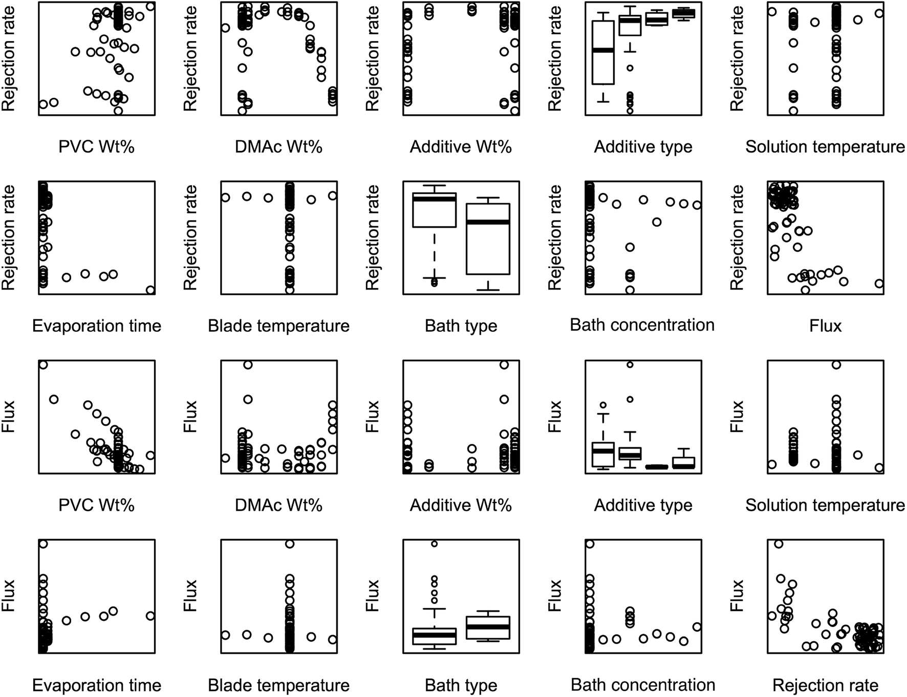 | ||
| Fig. 1 Scatter plots over measurements. | ||
3.2 Supervised learning and data analysis procedures
Furthermore, to estimate the accuracy of each SL algorithm, we apply the Monte Carlo method by repeating the learning processes 50 times on our measurement data. During each learning process, we first randomly split the data into a training set and a testing set, with the ratio 50/18. Next, we train each SL model based on the predictors of the training set with cross-validation and make predictions of responses over the training and testing sets using the trained learning model. Finally, we estimate the accuracy of each model by R-squared over the training and testing sets, computed as:
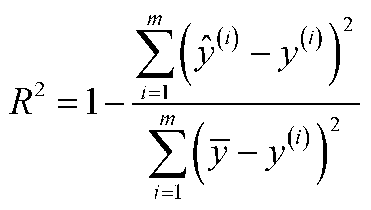 | (5) |
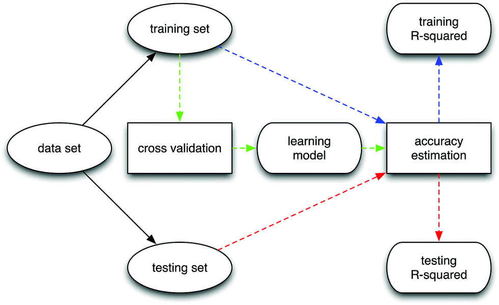 | ||
| Fig. 2 Data analysis procedure for each SL model, where ovals and rounded rectangles denote the input and estimated variables, respectively. | ||
3.2.2.1 Analysis of predictors' significance. According to LR analysis, the coefficients of PVC wt% and evaporation time, those of DMAc wt% and additive wt%, and those of additive and bath types are statistically significant at level 0, level 0.01, and level 0.05 for the rejection rate. However, there are only two statistically significant coefficients: one of PVC wt% at level 0 and another of DMAc wt% at level 0.1 for the flux. In other words, only a few processing parameters can provide significant information on the predictions; especially for the flux, PVC wt% and DMAc wt% are the two that carry the most amount of information. The low statistical significances are partially due to the small number of measurements. The linearity assumption on the relationship can be tested with R-squared values, which we will discuss later. In addition, the identical and independent distribution assumption on the noise can be tested by residual versus predicted response plots, which are shown in Fig. 3. Although the mean of residuals is indeed zero, the variance does not follow the null plot; this may be because our data is collected via a controlled parameter method.
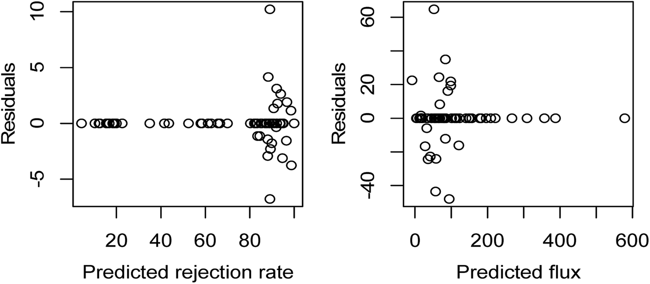 | ||
| Fig. 3 Residuals versus predicted values plots for rejection rate (%) and flux (L (m2 h)−1). | ||
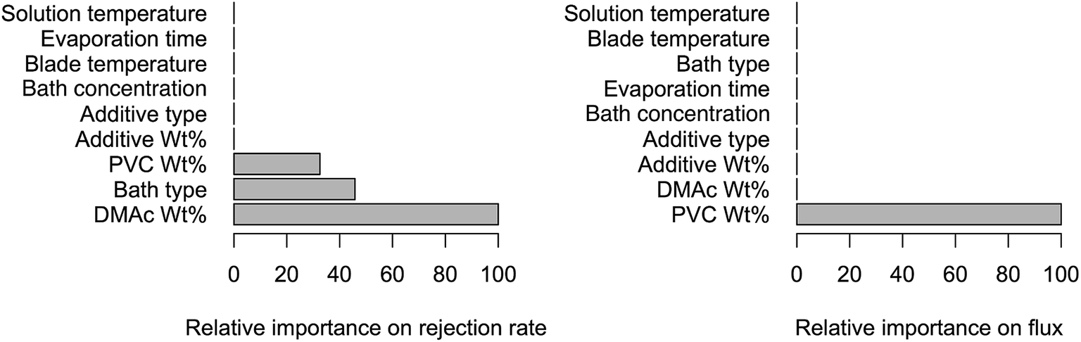
In case of MART analysis, the resulting importance rankings of each predictor for predictions are shown in Fig. 4. We can see that the number of significant predictors is even fewer than that in LR for each indicator. The importance order is DMAc wt% > bath type > PVC wt% for rejection rate, and only PVC wt% determines the regression tree for flux.
 | ||
| Fig. 4 Importance plots of predictors on each indicator. | ||
In summary, LR suggests that PVC wt% and DMAc wt% are the two most significant predictors. MART claims that the importance order of predictors is DMAc wt% > bath type > PVC wt% for rejection rate, while only PVC wt% determines the regression tree for flux. Based on the results of LR and MART, we remove the insignificant predictors (solution temperature) and then train NN and SVM with the appropriate controlling parameters determined by cross validation.
3.2.2.2 Selection of appropriate controlling parameters for NN and SVM. As shown in Fig. 1, the responses in our data are correlated, so NN is more appropriate than any other SL model, which can only predict the rejection rate and the flux separately. To apply NN, we should first assume that the categorical predictors (additive type and bath type) are numerical. In addition, we remove the unimportant predicator (solution temperature) and normalize all input predictors to zero-mean and one-standard-deviation.
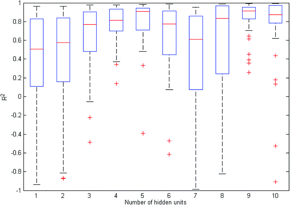
Furthermore, we select appropriate controlling parameters. Usually, one hidden layer is sufficient for a small training set. To select the optimal number of hidden units, we repeat the learning processes 50 times for each, and then select the one with a high mean and a low variance of testing R-squared values. During each process, we randomly split the data into a training set, a validation set, and a testing set, with the ratio 51/10/7, and then select the best number of epochs through cross-validation. The resulting box-plots are shown in Fig. 5. We can see the optimal number of hidden units is 9, with both the highest mean (0.8218) and the lowest variance of testing R-squared values.
 | ||
| Fig. 5 Box-plots of testing R-squared values over 50 training processes with different hidden layer sizes. | ||
As regard to SVM, since our data size is small, we select only the statistically significant 6 predictors in LR and MART to avoid overfitting. Furthermore, we choose the appropriate controlling parameters with five-fold cross-validation. The resulting support vectors are from all measurements except the 43rd or 18th measurements for the rejection rate or the flux, implying the risk of over-fitting.
4. Results and discussion
4.1 Performance of SL models and selections
The training and testing R-squared values of all SL models introduced above are listed in Table 1, where Rm and Rn denote the training and testing R-squared values, respectively, and y1 and y2 denote the rejection rate and the flux. We can see NN is the best SL model, with the highest Rm and Rn for both y1 and y2. The second best SL model is SVM, which performs considerably worse for y2 and Rn.| MART | NN | LR | SVM | |
|---|---|---|---|---|
| Rm(y1) | 0.2122 | 0.8897 | 0.6577 | 0.8065 |
| Rm(y2) | 0.0725 | 0.9175 | 0.6887 | 0.6583 |
| Rn(y1) | 0.0784 | 0.6344 | 0.3104 | 0.4344 |
| Rn(y2) | −0.0329 | 0.8093 | 0.1800 | 0.6583 |
By combining the performance results in Table 1 and the properties of each SL model, we can reveal some interesting underlying characteristics of the data. We begin with the worst SL model, MART, which has very low R-squared values for all conditions. In other words, the piecewise constant approximation does not work on this data, partially due to the small number of controlled measurements. However, we find that both the bias and variance are lower for the rejection rate. Thus, compared to the flux, the rejection rate has relatively high order interactions with processing parameters. This argument can be verified with the performance of LR. Both training R-squared values are relatively high. Especially for the flux, this value is even higher than that of SVM. Furthermore, SVM has much higher training R-squared of the rejection rate, and testing R-squared of both rejection and flux than those of LR. Therefore, the relationship between the flux and the processing parameters is approximately linear, but the rejection rate may have more complex and higher order interactions between the processing parameters. In addition, the noise of the measurement data is relatively high. Finally, although the testing R-squared values of SVM are much higher than LR due to the noise reduction in the higher dimensional feature space, they are still much lower than those of NN. This verifies the overfitting of SVM on small data, even when the regularization cost is set as high as 2.5
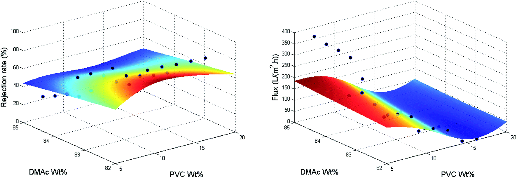
NN beats all other SL models in all aspects, and if the whole data is used for training, it has training R-squared values as high as 0.8992 and 0.9559 for the rejection rate and the flux. Thus, compared to the numerical approximation on categorical predictors, the correlation between the rejection rate and the flux is much more important in our predictions. To visualize the performance of NN, we plot the prediction versus the true response in Fig. 6. The performance is considered perfect if the point lies on the line with intersection 0 and slope 1. Furthermore, we plot the training data points and fitting curves of SVM and NN inside the predictor subspace of PVC wt% and DMAc wt% in Fig. 7 and 8 by fixing all other predictors as additive wt% = 0%, additive type = none, evaporation time = 5 s, blade temperature = 60 °C, bath type = water, and volume concentration of solute in gelation bath = 0 mg L−1. We can see that the fitting curves of NN are smoother and fit the training data better. In summary, because our data set is very small and noisy, the complex relationship between the rejection rate and the processing parameters is hard to fit with a good trade-off between bias and variance. Fortunately, we have the helpful information that tells us that it is correlated with the flux, which has a much simpler linear relationship, so we can apply NN to fit these two indicators.
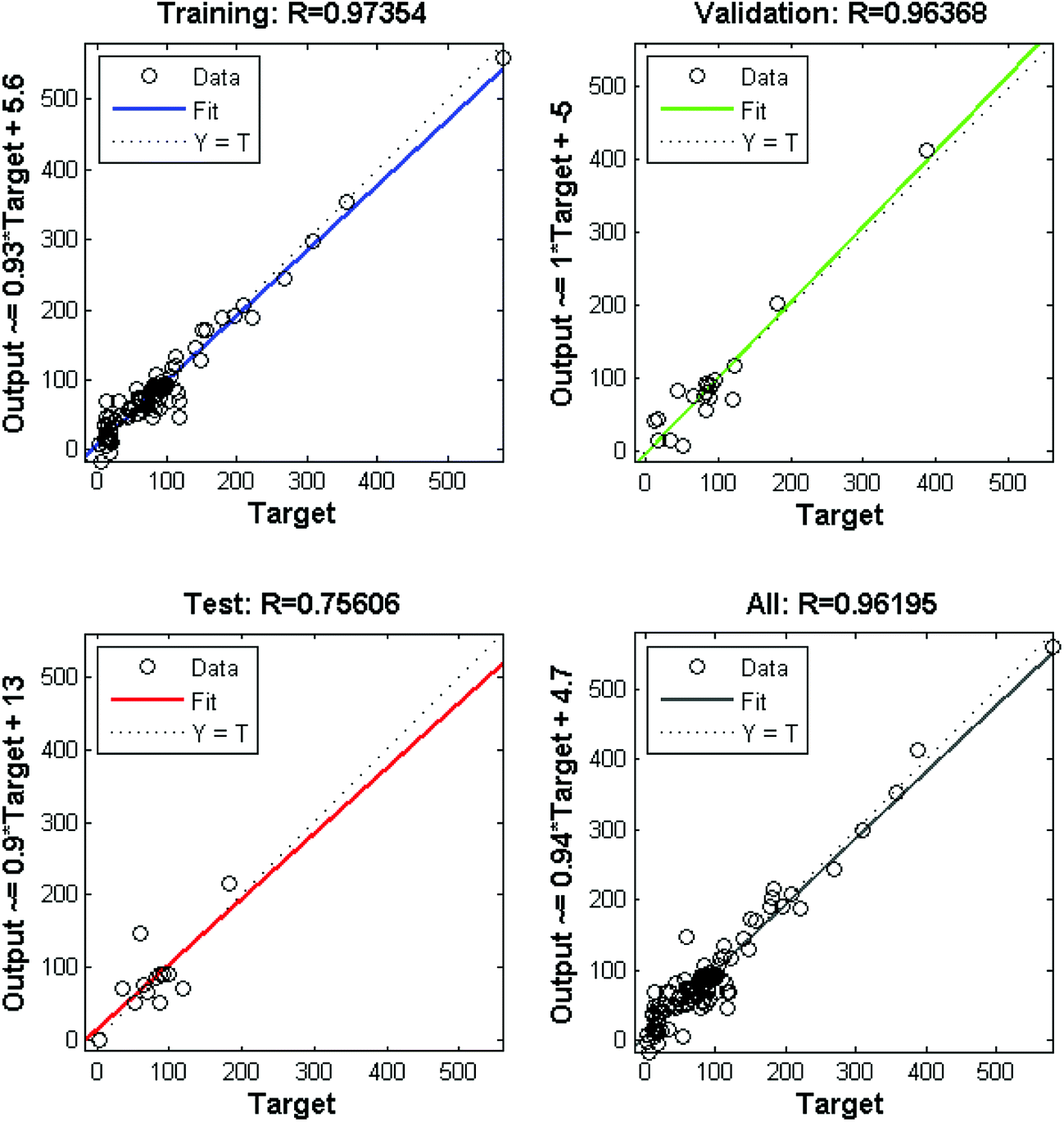 | ||
| Fig. 6 Prediction versus response plots for training, validation, testing, and the whole data set; target and output denote the true response and the predicted response by NN, respectively. | ||
 | ||
| Fig. 7 Training data and fitting curves of rejection rate and flux in the subspace of PVC wt% and DMAc wt% using SVM. | ||
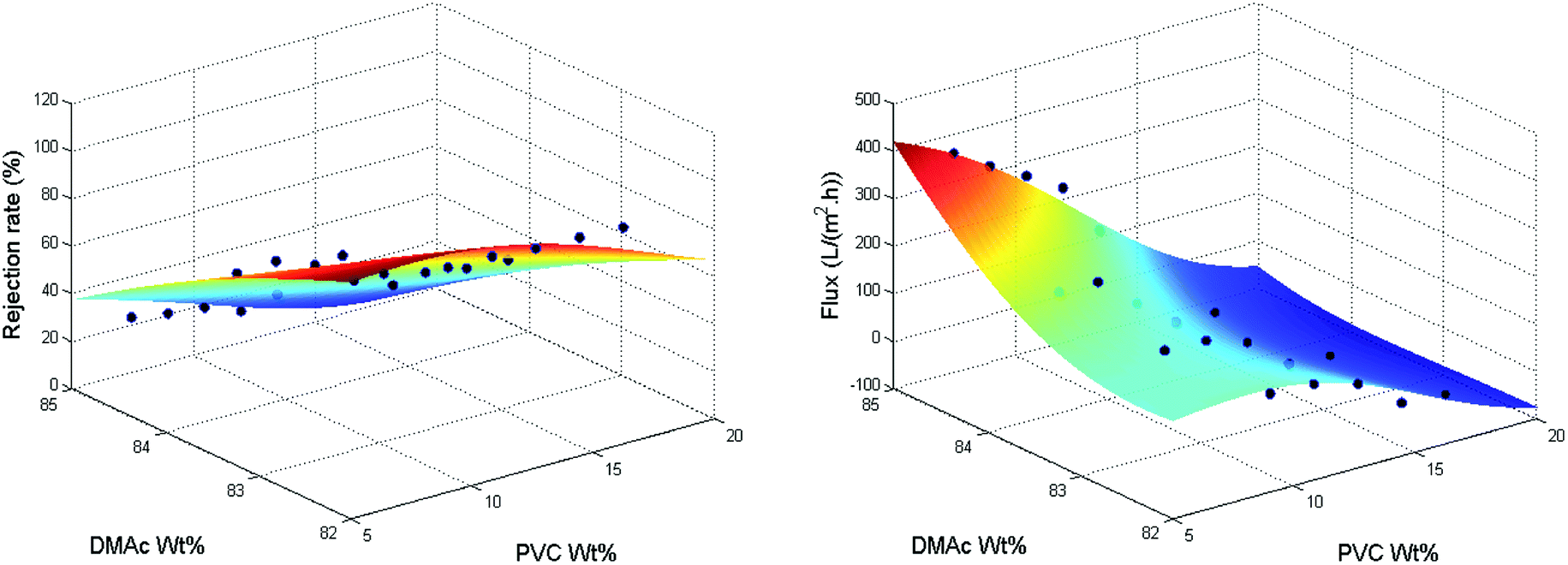 | ||
| Fig. 8 Training data and fitting curves of rejection rate and flux in the subspace of PVC wt% and DMAc wt% using NN. | ||
4.2 Optimization with NN
In this section, we use NN model to find the optimal combinations of processing parameters to maximize the flux under the constraint that the rejection rate of BSA should be no less than 80%. The idea is very simple: we search over the predictor space to find certain combinations that achieve the maximum predicted flux under the constraint regarding the predicted rejection rate by NN. For example, when we fix additive wt% = 1%, additive type = PEG600, evaporation time = 35 s, blade temperature = 70 °C, bath type = water, and bath concentration = 0 mg L−1, the possible combinations of PVC wt% and DMAc wt% satisfying rejection rate ≥ 80%, flux ≥ 200 L (m2 h)−1 are scattered in Fig. 9. It is noticed that the combinations are almost impossible in reality in the case of DMAc wt% < 40% or DMAc wt% > 85%. Therefore, a question is raised here on how to perform an efficient and reliable search. As a matter of fact, regarding to the problem, there exist two main difficulties: (1) when searching over a high-dimensional predictor space, the computation cost is very high; and (2) the predictions have high variance since the size of the training data is small. To overcome these difficulties, we first narrow down the search space by utilizing additional knowledge about the experiments and constraints on predictors. There are several obvious constraints, such as if additive type = none, then additive wt% = 0%; if bath type = water, then bath concentration = 0 mg L−1. In addition, our focus is on estimating how the addition of PVB into PVC improves the performance of membranes, so we introduce k as the ratio of PVC wt%/polymer wt%, giving us 0 < k < 1. Furthermore, we should keep the polymer wt% at no greater than 21%. Note that DMAc wt% can be easily calculated using eqn (3) and (4).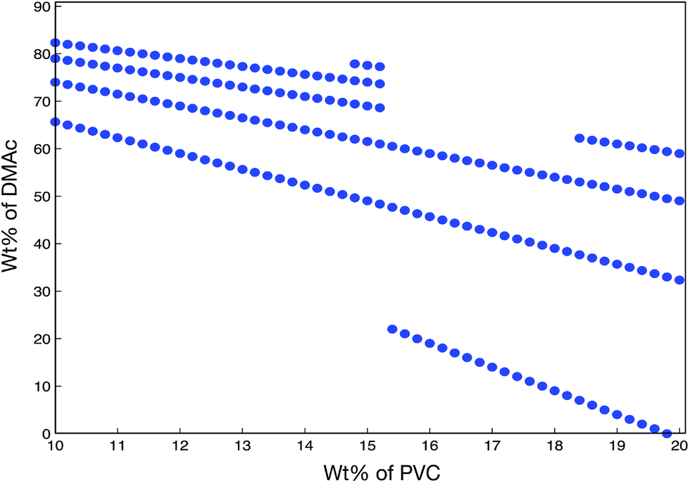 | ||
| Fig. 9 Possible combinations of PVC wt% and DMAc wt% for specific constraints on indicators fixing all other processing parameters. | ||
So we can use k instead of DMAc wt%. On the other hand, although the prediction accuracy is not guaranteed over the whole predictor space, both training and testing R-squared are very high within the data set. This means that if the search points are not too far away from the measurement points, the corresponding predictions are reliable. In particular, we have the search space PVC wt% = 7.5:0.5:18 (%), k = (PVC wt%/21), 0.05:0.9, and additive wt% = 1:1:5 (%) if additive type is not none, evaporation time = 5:15:110 (s), blade temperature = 30:10:80 (°C), and bath concentration = 10:10:80 (mg L−1).
Finally, we select the combination of processing parameters that have the maximum flux under the constraint 80% ≤ rejection rate ≤ 100%. We find with the water bath that the optimal combination of processing parameters is PVC wt% = 7.5%, DMAc wt% = 84%, additive wt% = 1%, k = 0.5 (PVB wt% = 7.5%), additive type = PEG600, evaporation time = 5 (s), and blade temperature = 30 (°C), leading to the rejection rate = 80.03% and the flux = 329.88 (L (m2 h)−1). Similarly, in the DMAc bath, we find that when PVC wt% = 16%, DMAc wt% = 78%, additive wt% = 2%, k = 0.8 (PVB wt% = 4%), additive type = PVP K90, evaporation time = 5 (s), blade temperature = 30 (°C), and bath concentration = 80 (mg L−1), we have the rejection rate = 81.39% and the maximum flux = 271.61 L (m2 h)−1. Although our results are not guaranteed to be globally optimal, they are much robust than the best measurement, which has the rejection rate = 82.07% and the flux = 122.70 L (m2 h)−1 (with the processing parameters PVC wt% = 12.6%, DMAc wt% = 77%, additive wt% = 5%, k = 0.7 (PVB wt% = 5.4%), additive type = PEG600, evaporation time = 10 s, blade temperature = 60 °C, bath type = DMAc, and bath concentration = 80 mg L−1). To check the accuracy of the models used to optimize membrane performance, we fabricated PVC/PVB flat sheet membranes strictly under the above optimized parameters. Fig. 10 shows the surface and cross-section morphology and the contact angle of the as-prepared membranes. In the case of pure water gelation bath, the rejection rate of the as-prepared membrane was 80.2% and the flux was 318.27 L (m2 h)−1, while in the case of DMAc as the solute of gelation bath, the as-prepared membrane has the rejection rate of 86.2% and the flux of 298.5 L (m2 h)−1. The results showed that there was a very good agreement between the model predictions and experimental data.
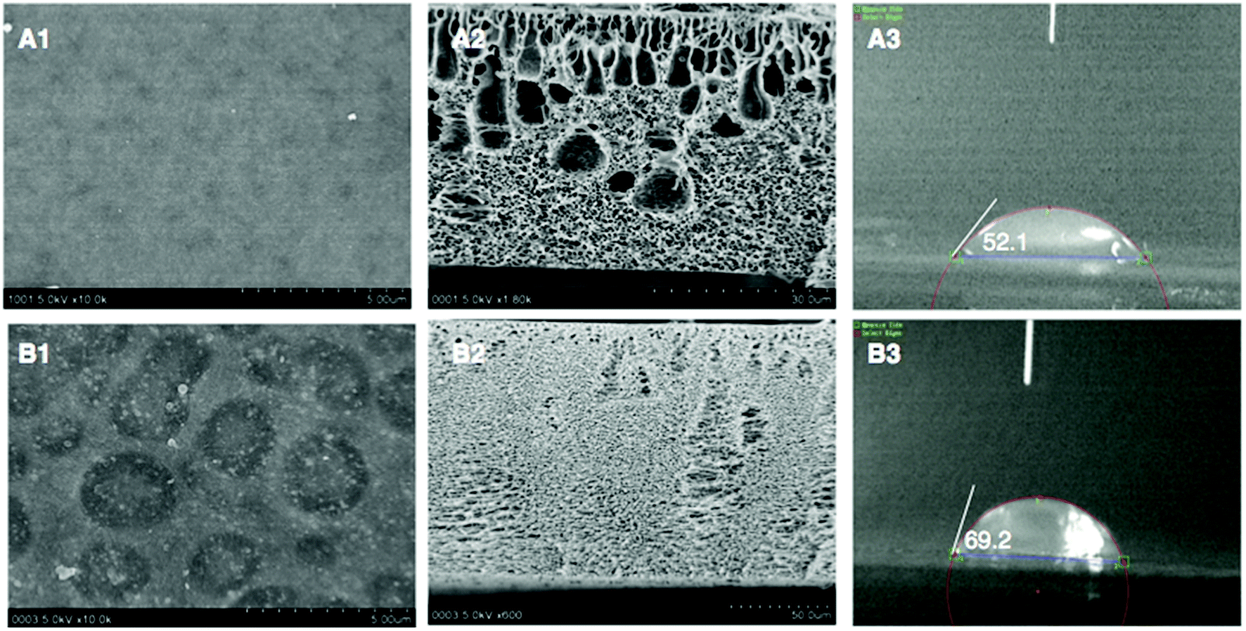 | ||
| Fig. 10 Morphology and the contact angle of PVC/PVB composite membranes ((A) the membrane prepared under optimized parameters in the case of using pure water as gelation bath, (B) the membrane prepared under optimized parameters in the case of using DMAc as the solute of gelation bath. (1) Surface structure (2) cross-section structure (3) contact angle). | ||
5. Conclusions
In this paper, we provide a systematical approach, namely, an SL-based framework for experimental data analytics, for modeling and optimizing membrane responses for complex combinations of membrane features during fabrication. This approach consists of the following procedures. First, control experiments are established to get various membranes with differing performances by combining various fabrication conditions. Second, the characteristics of the feature variables are analyzed in order to ascertain the quality of the data, as well as the data dependencies among the variables. Third, four SL approaches (MART, NN, LR, SVM) are employed to systematically analyze membrane performance and fabrication conditions in a rigorous fashion. Finally, the most reliable and trustful SL model is selected to optimize the fabrication conditions and predict the most favorable performance of PVC/PVB ultrafiltration membranes. During this last step, we analyze multiple responses simultaneously with multiple input feature variables. In this way, we eliminate most unnecessary assumptions that are traditionally proposed by other methods. In addition, this approach simplifies the analysis process by using a unified SL framework that has been thoroughly investigated by machine learning communities.24 This advantage surpasses previously reported DOE approaches in that these standard SL approaches provide smaller biases and variances for data analysis. Thus, the SL approaches offer us a more standard method not only in procedure but also with more rigorous results.Additionally, we glean several interesting findings from this research. One is how to find the optimal mixture of feature compounds for the fabrication processes more effectively and efficiently. Another is that among the tested SL approaches, the NN method provides the most reliable and trusted results. In the future, we will investigate how to develop a recursive and automated data-driven experimental analytics approach to design performance-specific membranes more effectively and efficiently.
Acknowledgements
We acknowledge financial support from the Division of International Cooperation & Exchange of Shanghai Jiao Tong University, China and the Newton Research Collaboration Award from Royal Academy of Engineering, UK (Reference: NRCP/1415/261). In addition, we are grateful to sponsors of the Center for Sustainable Development & Global Competitiveness (CSDGC) at Stanford University for additional financial support. Special thanks are given to the researchers at CSDGC for their technical support. Additionally, we thank Weimin Wu and Ting Wang for their valuable discussion.References
- S. Ramesh, A. H. Yahaya and A. K. Arof, Solid State Ionics, 2002, 148, 483–486 CrossRef CAS.
- Z. Yu, X. Liu, F. Zhao, X. Liang and Y. Tian, J. Appl. Polym. Sci., 2015, 132, 41267 Search PubMed.
- N. Wang, A. Raza, Y. Si, J. Yu, G. Sun and B. Ding, J. Colloid Interface Sci., 2013, 398, 240–246 CrossRef CAS PubMed.
- S. Chuayjuljit, R. Thongraar and O. Saravari, J. Reinf. Plast. Compos., 2008, 27, 431–442 CrossRef CAS.
- M. Jakic, N. S. Vrandecic and I. Klaric, Polym. Degrad. Stab., 2013, 98, 1738–1743 CrossRef CAS.
- X. Zhao and N. Zhang, Journal of Tianjin University Science and Technology, 2007, 22, 36–39 Search PubMed.
- J. zhu, L. Chi, Y. Zhang, A. Saddat and Z. Zhang, Water Purif. Technol., 2012, 31, 46–54 CAS.
- Y. Peng and Y. Sui, Desalination, 2006, 196, 13–21 CrossRef CAS.
- Y. Sui, Thesis for Master Degree, Beijing University of Technology, Beijing, China, 2004, pp. 24–26.
- X. Zhao and K. Xu, Plast. Sci. Technol., 2010, 1–6 Search PubMed.
- E. Corradini, A. F. Rubira and E. C. Muniz, Eur. Polym. J., 1997, 33, 1651–1658 CrossRef CAS.
- S. Y. L. Leung, W. H. Chan and C. H. Luk, Chemom. Intell. Lab. Syst., 2000, 53, 21–35 CrossRef CAS.
- S. Y. Lam Leung, W. H. Chan, C. H. Leung and C. H. Luk, Chemom. Intell. Lab. Syst., 1998, 40, 203–213 CrossRef CAS.
- W. H. Chan and S. C. Tsao, Chemom. Intell. Lab. Syst., 2003, 65, 241–256 CrossRef CAS.
- M. Khayet, C. Cojocaru, M. Essalhi, M. C. García-Payo, P. Arribas and L. García-Fernández, DES, 2012, 287, 146–158 CrossRef CAS.
- L. Wenjau and O. Soonchuan, Computer and Automation Engineering (ICCAE), 2010 The 2nd International Conference, 2010, vol. 2, pp. 50–54 Search PubMed.
- P. W. Araujo and R. G. Brereton, Trends Anal. Chem., 1996, 15, 63–70 CAS.
- K. I. Wong, P. K. Wong, C. S. Cheung and C. M. Vong, Energy, 2013, 55, 519–528 CrossRef.
- Y. Reich and S. V. Barai, Artif. Intell. Eng., 1999, 13, 257–272 CrossRef.
- B. L. Whitehall, S.-Y. Lu and R. E. Stepp, Artif. Intell. Eng., 1990, 5, 189–198 CrossRef.
- F. J. Alexander and T. Lookman, Novel Approaches to StatisticalLearning in Materials Science, Informatics for Materials Science and Engineering, 2013 Search PubMed.
- S. S. Madaeni, N. T. Hasankiadeh, A. R. Kurdian and A. Rahimpour, Sep. Purif. Technol., 2010, 76, 33–43 CrossRef CAS.
- X. Xi, Z. Wang, J. Zhang, Y. Zhou, N. Chen, L. Shi, D. Wenyue, L. Cheng and W. Yang, Desalin. Water Treat., 2013, 51, 3970–3978 CrossRef CAS.
- C. M. Bishop, Pattern Recognition and Machine Learning, Springer Verlag, 2006 Search PubMed.
Footnote |
| † Electronic supplementary information (ESI) available. See DOI: 10.1039/c5ra24654g |
| This journal is © The Royal Society of Chemistry 2016 |