Modeling the atomistic growth behavior of gold nanoparticles in solution

Abstract

The properties of gold nanoparticles strongly depend on their three-dimensional atomic structure, leading to an increased emphasis on controlling and predicting nanoparticle structural evolution during the synthesis process. In order to provide this atomistic-level insight and establish a link to the experimentally-observed growth behavior, a kinetic Monte Carlo simulation (KMC) approach is developed for capturing Au nanoparticle growth characteristics. The advantage of this approach is that, compared to traditional molecular dynamics simulations, the atomistic nanoparticle structural evolution can be tracked on time scales that approach the actual experiments. This has enabled several different comparisons against experimental benchmarks, and it has helped transition the KMC simulations from a hypothetical toy model into a more experimentally-relevant test-bed. The model is initially parameterized by performing a series of automated comparisons of Au nanoparticle growth curves versus the experimental observations, and then the refined model allows for detailed structural analysis of the nanoparticle growth behavior. Although the Au nanoparticles are roughly spherical, the maximum/minimum dimensions deviate from the average by approximately 12.5%, which is consistent with the corresponding experiments. Also, a surface texture analysis highlights the changes in the surface structure as a function of time. While the nanoparticles show similar surface structures throughout the growth process, there can be some significant differences during the initial growth at different synthesis conditions.

---

1. Introduction

The current applications of gold nanoparticles span a broad variety of technical platforms, ranging from optical and catalytic systems^1–6 to data storage and biomedical applications.^7–11 As the applications for nanomaterials continue to steadily expand, there has been an increased emphasis on controlling and predicting nanoparticle formation (size, morphology, and composition). This fundamental interest is motivated by the fact that many of the unique nanomaterial properties are strongly correlated to subtle changes in the nanoparticle structure and surface termination.¹² Thus, there is much to be gained by developing experimental protocols for reliably producing specific nanoparticle morphologies. Moreover, developing larger-scale processes for generating the same quality of nanomaterials is particularly important for translating these laboratory discoveries to commercial applications. Here, we specifically focus on modeling the solution-phase growth of Au nanoparticles, due to their diverse applications and the availability of relevant experimental synthesis details.

In order to accelerate the field of Au nanoparticle production and shape control, many experimental and modeling studies have been performed to help clarify the underlying nanoparticle formation mechanisms^13–18 and expected material properties.^10,19,20 With a deeper fundamental understanding of these issues, progress in this field can be accelerated and more rational synthesis recipes can be devised. In terms of the modeling work, a diverse set of theoretical approaches have been taken in the past, ranging in scale from quantum mechanical investigations of detailed reaction steps and energetics^{16,17,21–25} to continuum models^18,26–30 for predicting dynamic growth behavior (consistent with laboratory time and length scales). As with any modeling approach, these examples from the literature represent tradeoffs between model resolution and computational efficiency. Studies conducted with density functional theory (DFT) can provide quantitative estimates of isolated values, such as Au–ligand surface binding or the relative thermodynamic stability of small Au clusters.^31,32 On the other hand, continuum level models can be parameterized to fit experimental growth behavior and rationalize different trends, but this is obtained by sacrificing atomistic resolution. Overall, one of the most daunting, yet critically important, challenges is to model nanoparticle growth behavior with atomistic resolution on time scales that approach the experimental observations. This is a gap in the modeling hierarchy that has not been adequately addressed.

In many examples from the literature, molecular dynamics (MD) simulations are able to capture the necessary atomistic features, but their inherently short timescales can limit their range of applicability. In some situations, advanced sampling methods can enhance the exploration of phase space in traditional MD simulations, and this includes methods such as parallel tempering,³³ umbrella sampling,³⁴ or metadynamics.^35,36 For instance, Rossi and Baletto³⁷ provide an example of applying metadynamics to explore the structural transitions of monometallic (Ag, Pt) and bimetallic (Ag/Pt) clusters, and other MD-based examples have helped identify the low-lying energy configurations of various metal clusters.³⁸ However, the inability to track long-time kinetic behavior is still a challenge.

In order to provide additional atomistic-level insight and establish a link to the experimentally-observed growth behavior, we have implemented a kinetic Monte Carlo (KMC)^39–43 approach for capturing Au nanoparticle growth characteristics. There have been many previous applications of KMC to model the kinetics of nanoscale phenomena, including crystal growth of urea from solution,⁴⁴ nanoparticle coalescence,⁴⁵ electrochemical systems,^46–50 and several examples in the area of thin film deposition^51–56 and heterogeneous catalysis.^57–60 In brief, the KMC method can provide an estimate of the time evolution of Markovian processes,⁴⁰ as long as there is an accurate set of transition rates characterizing the simulated processes, which are assumed to obey Poisson statistics.⁶¹ While additional modeling details are provided in the next section, our current KMC implementation should be viewed as semi-quantitative, due to the inherent uncertainty of several of the system parameters and ambiguity about the exact steps in the underlying Au nanoparticle growth mechanism. With additional applications of the model and further experimental benchmarking, it is expected that more quantitative reliability can be obtained and more fundamental insight can be gained.

There have only been a few previous attempts to use KMC to model nanoparticle growth. Haldar and Chatterjee⁶² provide a very recent example of modeling the dynamics of a small Ag cluster on an Ag(001) surface, and their model was built around a rigorous KMC rate database that was generated with basin-constrained MD simulations.⁶³ Also, Gorshkov et al.^64,65 have previously used KMC to model the general growth behavior of colloids, nanoparticles, and core–shell nanoparticles. A range of different nanoparticle shapes were generated, and interesting surface features were predicted (such as surface clustering on core–shell systems). However, these examples are referred to by the authors as “cartoons”, since arbitrary system parameters were used (not intended to mimic a real system). Regardless of some uncertainty in the parameterization details, the KMC approach can provide an improvable modeling framework that can be used to directly connect the experimental synthesis conditions (temperature, precursor concentration, growth time, etc.) to the atomistic features of the final nanoparticle structures.

Here, our goal is to extend the KMC technique to simulate the growth dynamics of the solution-phase synthesis of Au metal nanoparticles. Such a model can provide direct information about the impact of individual system events on the final atomic-scale structural features of the Au nanoparticles, and this can help guide the experimental synthesis process. In order to develop a reasonable set of model parameters, several experimental benchmarks are taken from the literature and used to train the KMC model, and this is followed by a sensitivity analysis of the growth behavior on the underlying kinetic parameters. While quantitative predictability is not expected at this stage, we provide the first example of applying atomistic KMC to mimic the experimental behavior of Au nanoparticle growth from solution. With this model, we provide detailed information about the Au nanoparticle structure as a function of synthesis conditions, and this analysis includes an evaluation of the nanoparticle geometry and atomic-level surface features. Due to the inherent computational efficiency of our approach, there are future opportunities to extend the KMC model to include many other reaction steps or events in the formation mechanism to capture additional experimental influences on the final nanoparticle structure. Here, we report the effects of synthesis temperature and precursor concentration on the Au nanoparticle growth behavior, and we find that our model can be trained to adequately reproduce the experimental growth curves at the same conditions. With detailed computational analysis of the nanoparticles, we are able to track their morphological evolution as a function of time, including max/min dimensions, surface area/volume, and surface structural characteristics.

2. Computational methods and model

In our KMC simulations, the conditions have been chosen to follow a previous experimental study.¹⁴ Thus, the initial Au⁺ salt concentration is specified, and the reducing agent R (t-butylamineborane) is initially present in the solution at a concentration of 10× the Au⁺ concentration. In the experiments, the synthesis temperature ranges from 23 to 45 °C, and the solvent is toluene with a dodecanethiol stabilizer. According to these conditions, the reduction of Au⁺ is assumed to occur in the bulk solution, followed by deposition to the nanocluster surface. The total amount of Au⁰ available for deposition is dictated by the initial concentration of Au⁺ and the volume of the effective bulk solvent bath. During the course of the simulation, the total number of atoms is conserved: Au⁺(bulk) + Au⁰(bulk) + Au_N(nanoparticle). The bath volume is assumed to be correlated to the average nanoparticle–nanoparticle separation distance in the experimental system, which determines the local availability of adsorbates. In our systems, the bath volume (corresponding to one Au cluster) ranges from ∼8 to 13 × 10⁶ nm³, or a box length of 94 to 115 nm.

With such a complex experimental system, involving many steps and sophisticated mechanisms, it is unrealistic to expect that the experimental growth process will be fully captured in our model. For instance, we do not explicitly model features such as the nanoparticle nucleation events, concentration gradients in the solution, pH, or stabilizing ligands. While all of these factors can have a strong influence on the nanoparticle growth process, these factors often translate into contributions to the growth kinetics. Thus, in the absence of a comprehensive set of benchmark data over a wide range of different conditions, we have adopted a minimal event database for modeling the mechanism of the Au nanoparticle growth. As a result, the individual rate parameters should be interpreted as semi-empirical average values for a particular event (which encompass the influence of the specific system conditions mentioned above). Currently, the following events and rate expressions shown in Table 1 are included in the KMC growth mechanism, where the brackets indicate molar concentration.

Table 1 Summary of events and event rates included in the Au growth mechanism

Event	Rate expression
Au^0 surface diffusion on nanoparticle	r diff = kdiff·exp((−Ea,diff − (Ei − Ef))/(2kBT))
Au^0 desorption from nanoparticle	r des = kdiff·exp((−Ea,diff − Ei)/(2kBT))
Au^0 adsorption on nanoparticle	r ads = kads[Au^0]
R consumption in bulk	d[R]/dt = −kred[Au^+][R]
Au^+ reduction to Au^0 in bulk	d[Au^+]/dt = −kred[Au^+][R]
Au^0 concentration in bulk	d[Au^0]/dt = kred[Au^+][R] + rads − rdes

---

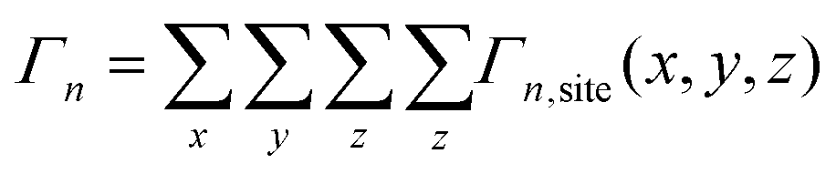
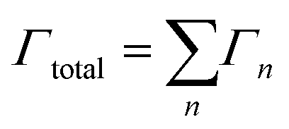
Starting from an isolated Au nanoparticle seed and a given set of simulation conditions (temperature, precursor concentration, etc.), the system is propagated through time by implementing a KMC algorithm, along with the pre-specified database of energetic and rate information (Table 1). Thus, starting from the initial system configuration on an FCC lattice, the rate (Γ_n,site) of each event (n) is calculated at each lattice site (x, y, z), which gives a net event rate of Γ_n, and the total rate of all events in the system is Γ_total.

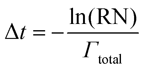
After the system configuration has been defined and the initial rates have been calculated, the system clock is then advanced according to the following equation, where Δt is the time step and RN is a random number, evenly distributed between 0 and 1.

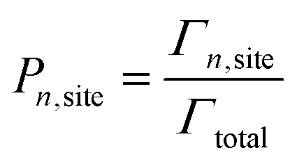
After the clock has been incremented, the system configuration is then updated by stochastically choosing an event to occur, according to the probability shown in eqn (4). Once an event is identified to occur, the system configuration is updated, and the list of event rates is updated (according to the new configuration). At each time step, an event is always performed.

The dimensions of the simulation box are large enough to prevent self-interactions during the growth of the Au nanoparticles generated in our study. Thus, our simulations do not allow for particle–particle interactions, which may ultimately lead to clustering behavior or ripening phenomenon. At the growth conditions chosen, the corresponding experiments have indicated that these interactions are insignificant,¹⁴ so only isolated Au nanoparticles are considered in our current modeling work.

In the simulations, several different basic KMC moves are allowed (adsorption, surface diffusion, desorption), and the moves on the growing cluster will depend upon the local energetics. The energy of different configurations is approximated by counting the local coordination of each atom (first-neighbor and next-nearest-neighbor), and each neighbor contributes a value of −4 kcal mol⁻¹ to the total energy. While these energy values are simple approximations, the total energy values in the KMC simulations fall within typical ranges of Au binding energies (∼48 kcal mol⁻¹ in small clusters³² to ∼80 kcal mol⁻¹ for Au on periodic Au(110) and Au(100) surfaces⁶⁶). In future work, our energy values could be made more quantitative by introducing a many-body potential energy function,⁶⁷ or more accurately, by performing dedicated electronic structure calculations specific to our system. In fact, previous reports have indicated that many-body potentials (often fit to bulk metal behavior) can produce significant errors, especially when modeling nanoparticles or surfaces.⁶⁸ Thus, due to the highly corrugated surface of small nanoparticles, electronic structure calculations would be the preferred route for generating reliable improvements to our estimated energy value. In addition, this would potentially allow for a clearer accounting of the role of surface ligands on the energetics.

As the nanoparticle grows and as the Au atoms redistribute on the nanoparticle surface, the local event rates are continually recalculated and updated. For diffusion events, the change in total energy resulting from a move is used to calculate the event rate, as well as a baseline activation barrier. According to the expressions in Table 1, E_i is the energy at the initial position, E_f is the energy at the final position, and E_a,diff is the baseline activation energy. The value for E_a,diff is estimated at 35 kcal mol⁻¹. Previous calculations had estimated the activation barrier to be ∼5 to 20 kcal mol⁻¹ on smooth Au surfaces,^66,69 so in the present work, the barrier was increased to reflect the significant increase in roughness corresponding to the dynamic nanoparticle surface. Consistent with many previous modeling studies,^69–71 the pre-exponential factor for the Au⁰ diffusion is estimated to be 10¹³ s⁻¹.

The KMC adsorption/desorption of the Au atoms are coupled to an implicit solution bath, which changes composition with time by synchronizing the differential equations describing the reaction events in the bath (shown in Table 1) with the KMC system clock. At each KMC step, the system clock is incremented, and this small time step is used to numerically integrate the differential equations forward in time from the previous state. While the time steps in KMC are variable, they are small enough that the integration is stable and accurate. In the simulation, the implementation is a simple accounting of the number of free Au atoms in the solution bath. According to the total size of the simulation box and the initial Au concentration in the bulk solution, the time-dependent number of Au atoms present in the bulk increases/decreases with respect to each desorption/adsorption move from/to the Au nanoparticle surface, and the bulk Au concentration increases as the Au⁺ precursor is reduced (according to the pre-defined rate equation). By coupling the composition of the bulk solution to the Au nanoparticle growth kinetics, the nanoparticle growth naturally attenuates as the bulk solution becomes depleted of precursor species. Desorption of Au⁰ atoms occurs when an Au⁰ atom of the nanocluster is displaced away from the nanocluster, resulting in the absence of any nearest-neighbors. If an Au atom is detached from the nanoparticle by a displacement move, its explicit identity and location are lost and it is absorbed into the bulk fluid (with the analytical bulk concentration adjusted accordingly).

3. Results and discussion

The overall mechanism adopted here is similar to the analytical model recently developed by Chen et al.,¹⁴ who compiled theirs from various sources of experimental data. However, a number of simplifications have been imposed (i.e., neglecting an accounting of the solid–fluid interfacial tension, the initial nucleation process, bulk diffusion limitations, etc.), and the explicit treatment of Au atom diffusion on the nanoparticle surface has been introduced in our model. As a result, in contrast to the previous study, our model is not limited to smooth spherical Au nanoparticles. Instead, we preserve the atomistic features of the Au nanoparticle growth (edges, corners, etc.), including an accounting of individual Au atom displacements and restructuring on the growing nanoparticle surface. While not encountered in this work, this allows us to potentially model the anisotropic growth of nanorods, tetrapods, cubes, etc.

In the Au formation mechanism adopted, the values of the rate parameters corresponding to the reactions in Table 1 have been adjusted from previous analytical models,¹⁴ in order to match the available experimental growth data. As such, the transferability of these parameters to different growth conditions (solvent, pH, precursors, etc.) will certainly result in quantitative errors, and likely, qualitative discrepancies. While this is undesirable, the ability to make such comparisons is important. By exploring additional experimental conditions, there are excellent opportunities for expanding and improving upon the basic mechanistic steps in the KMC simulations. Thus, as additional experimental benchmarks become available, this allows a progressive and deeper fundamental understanding of the connections between experimental phenomena and atomic-level nanoparticle synthesis.

3.1 Experimental benchmarking

In order to refine the rate constants adopted in our KMC model, we performed simulations of nanoparticle growth rate versus time and compared our results to the corresponding experimental data.¹⁴ Several different sets of conditions were explored (shown in Table 2), and the rate constants were adjusted to minimize the error between the predicted and experimental curves. Since the initial nanoparticle nucleation process was not captured in our model, the size of the initial Au nanopaticle seed was chosen to best match the experimental data at the various conditions. Due to the inherent computational efficiency of our KMC simulations, the Au nanoparticle growth process and simultaneous shape analysis can typically be completed within a few minutes on a single computer processor core. This allows for a wide range of conditions and parameters to be rapidly explored, and in particular, it highlights the opportunity for an automated feedback comparison loop with respect to the experimentally-observed nanoparticle growth data. Thus, these simulations were fed the experimental growth curves as the target, and the simulations automatically iterated through a process of nanoparticle growth, error analysis, and parameter adjustment until satisfactory convergence was obtained.

Table 2 Optimized parameter values corresponding to different experimental conditions

Reaction conditions	k ads [L (mol s)^−1]	k red [L^2 (mol^2 s)^−1]	Volume [nm^3]
T = 23 °C, [Au^+]0 = 12.5 mM	0.272	2.822 × 10^−3	8.329 × 10^5
T = 33 °C, [Au^+]0 = 12.5 mM	1.108	3.586 × 10^−3	1.096 × 10^6
T = 45 °C, [Au^+]0 = 12.5 mM	3.529	4.729 × 10^−3	1.540 × 10^6
T = 23 °C, [Au^+]0 = 10.0 mM	0.272	2.822 × 10^−3	8.254 × 10^5
T = 23 °C, [Au^+]0 = 7.5 mM	0.382	4.220 × 10^−3	8.403 × 10^5
T = 23 °C, [Au^+]0 = 5.5 mM	0.302	2.323 × 10^−3	1.368 × 10^6

---

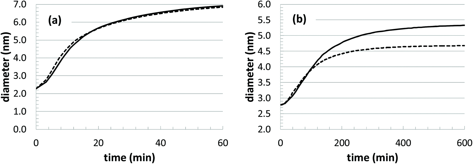
During our optimization procedure, three different parameters (k_ads, k_red, and solvent volume) were adjusted, in order to minimize the standard deviation between the experimental and computed nanoparticle growth curves at different conditions. Although the final solutions may not be unique, the parameter values are well-bounded, and multiple optimization attempts led to similar convergence after approximately 10–20 individual perturbations of each parameter. The growth curves resulting from the optimization are shown in Fig. 1 and 2, with the corresponding parameter values listed in Table 2.

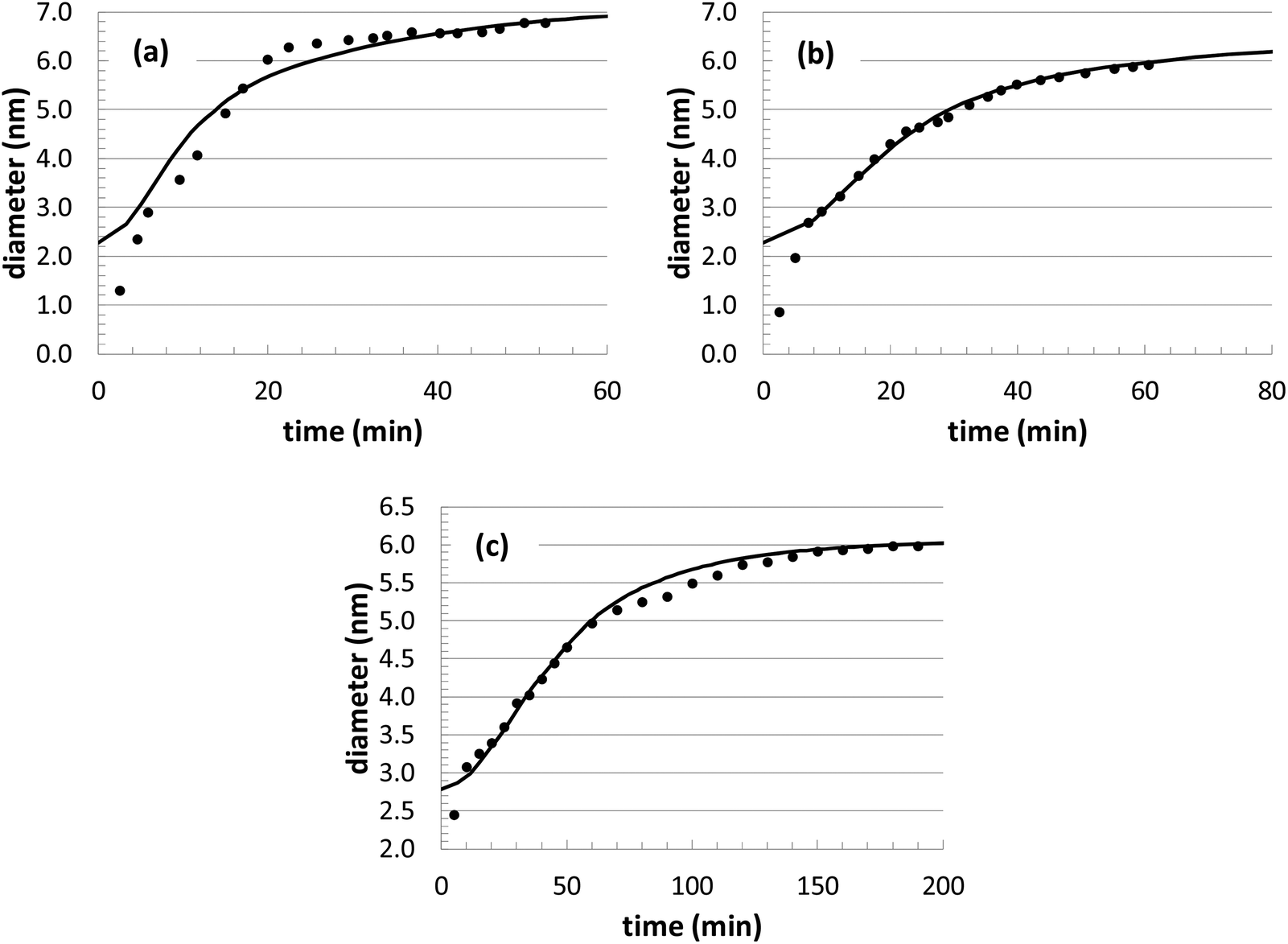Fig. 1 Comparison of KMC simulation of Au nanoparticle growth with previous experiments at three different temperatures: (a) T = 45 °C; (b) T = 33 °C; (c) T = 23 °C. In all cases, the [Au⁺]₀ precursor concentration is 12.5 mM. The solid curves are the simulations and the black circles are the experiments.

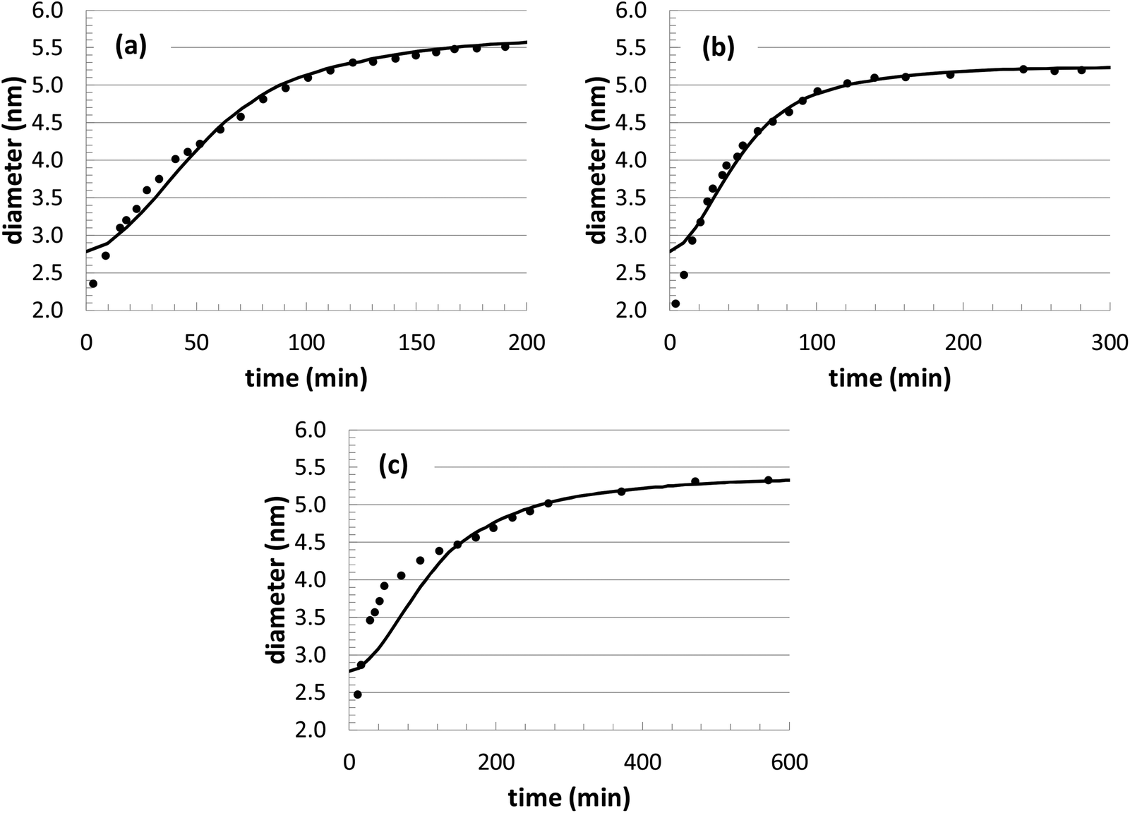Fig. 2 Comparison of KMC simulation of Au nanoparticle growth with previous experiments at three different [Au⁺]₀ precursor concentrations: (a) 10.0 mM; (b) 7.5 mM; (c) 5.0 mM. In all cases, the temperature is 23 °C. The solid curves are the simulations and the black circles are the experiments.

In theory, it would be ideal to obtain a unique set of parameters that can capture the Au nanoparticle growth behavior over a wide range of conditions. However, with our current model, the parameters adopt different values at different conditions. This variability was also found when an analytical model was used to describe the growth behavior of this same system.¹⁴ With respect to the growth behavior at different temperatures (Fig. 1), the model results are actually very consistent. As expected, the reaction rate values increase significantly with respect to temperature, leading to a general Arrhenius expression for the rate constant. Although only 3 different temperatures are explored, both rate constants (k_ads and k_red) can be fit to an Arrhenius plot, with a correlation coefficient of over 0.99. This leads to predicted activation energies of 21.7 kcal mol⁻¹ for k_ads and 4.4 kcal mol⁻¹ for k_red. The value of k_ads is in very good agreement with the previous analytical modeling result of 20.3 kcal mol⁻¹. Also, it is consistent with the binding energy of long-chain thiols to Au nanoparticles of 20.4 kcal mol⁻¹,⁷² which is assumed to correspond to the energetics of nanoparticle growth. The value of k_red is somewhat lower than other related literature values for the reduction of Au³⁺ with a borohydride BH₄⁻ complex (12.4 kcal mol⁻¹),⁷³ dimethylamine borane (9.5 kcal mol⁻¹),⁷⁴ or NaHSO₃ (7.4–9.1 kcal mol⁻¹).⁷⁵

The nanoparticle growth curves with the different initial precursor concentrations (Fig. 2) demonstrate more unpredictability. The rate parameter values are all within 10% of each other over this range of conditions, except for the experiments performed at an [Au⁺]₀ value of 7.5 mM. There are several different possible sources for the anomalous behavior, given the complex reaction environment in the experiments and the simplified mechanism adopted in our model. At different concentrations, there can be shifts in the competition between nanoparticle growth and nucleation events, there can be inherent changes in the mechanism (i.e., promoting Au⁺ reduction at the nanoparticle surface versus in the bulk solvent), and there could be unexpected nanoparticle aggregation or dissolution events. While the interplay of these different factors is currently unknown for our particular system, these steps could be explicitly included in our future KMC modeling work in order to identify the roles of these competing mechanisms.

3.2 Geometrical analysis

During the course of the simulation, several different instantaneous metrics are evaluated, in order to quantify the geometric details of the Au nanoparticle shape evolution. Although we do not have experimental benchmarks with which to compare, these features can play important roles in the final material performance (catalytic, optical, etc.). In our analysis, we track the time evolution of the maximum/minimum particle dimensions, total volume, surface area, and the local coordination of the surface atoms.

In Fig. 3, we illustrate the maximum and minimum shape dimensions relative to the average diameter, as a function of time. The average diameter value is simply calculated by using the total nanoparticle volume and assuming a spherical shaped particle. In the graph, three different temperatures are shown, and all three reach the same average value after approximately 20 minutes of growth. The higher temperature converges more quickly than the lower temperatures, but when the [Au⁺]₀ precursor concentration is varied, there is no noticeable change in convergence (data not shown). Interestingly, the final average value of ∼12.5% in the KMC simulations is very close to the range of polydispersity observed in the experiments of ∼10–13%.¹⁴

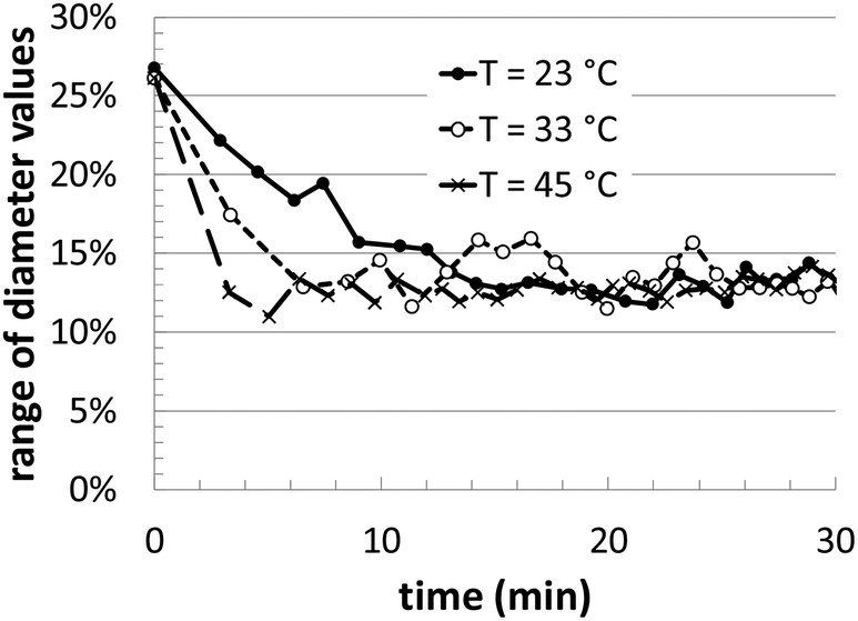Fig. 3 Range of diameter values calculated from simulation, taken as the deviation of the maximum and minimum shape dimensions relative to the average diameter. The lines correspond to three different temperatures, as indicated, all with a [Au⁺]₀ of 12.5 mM.

Fig. 4 presents related structural information. In the plot, we compare the surface area/volume ratio of one of the Au nanoparticles (T = 23 °C and [Au⁺]₀ = 12.5 mM) to an ideal sphere of the same volume. This provides an estimate of deviations in the surface structure, which might include asphericity, surface roughness, etc. Although our Au nanoparticles are approximately spherical, this analysis highlights the presence of geometrical deviations, which are also reflected in Fig. 3. In particular, this analysis can be especially useful for computationally searching for growth conditions that produce branched nanoparticles (possessing very high surface to volume ratios).

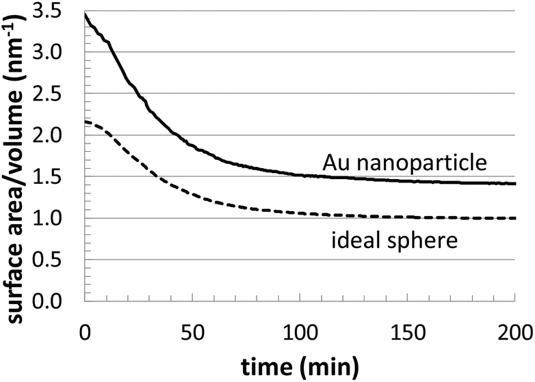Fig. 4 Comparison of the evolution of the surface/volume ratio for a simulated Au nanoparticle (T = 23 °C and [Au⁺]₀ = 12.5 mM) versus and ideal sphere of the same volume.

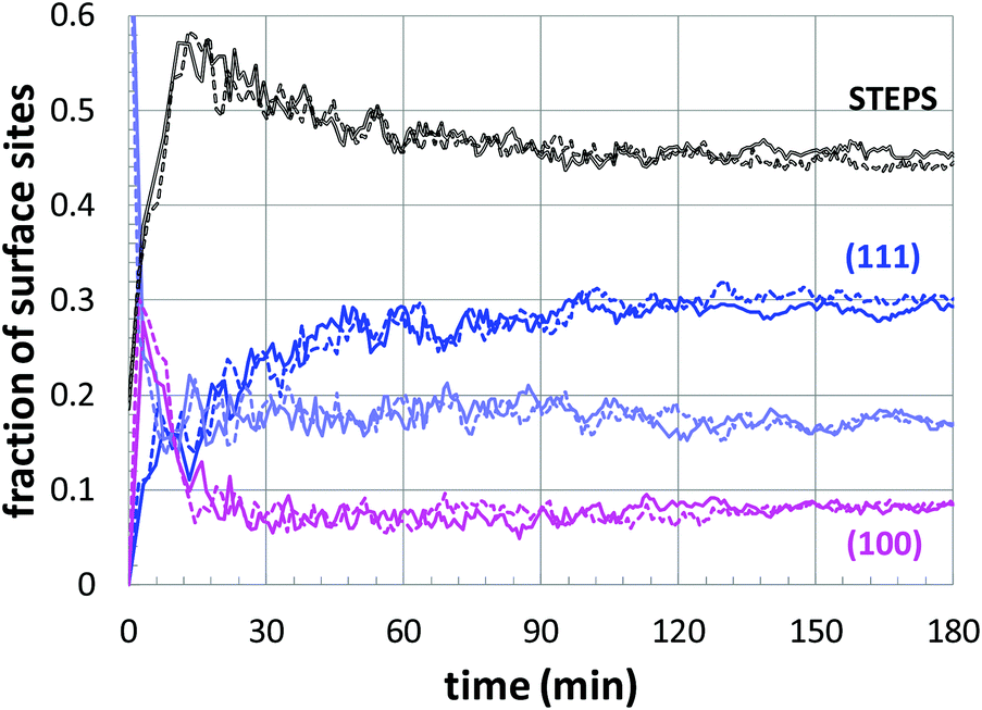
Next, a more detailed analysis of the nanoparticle surface was performed, in order to develop a more quantitative description of the surface structure. In the KMC simulations, the instantaneous nanoparticle configurations were analyzed by performing a neighbor analysis of each surface atoms, and each atom was classified according to its local coordination. The primary classifications identified are (100) sites, (111) sites, and steps/edges. This analysis is illustrated in Fig. 5, which shows an instantaneous snapshot of one of the growing Au nanoparticles corresponding to a synthesis temperature of 23 °C and an initial [Au⁺]₀ of 12.5 mM. In Fig. 6, the time evolution of the surface sites is illustrated. While different synthesis conditions lead to similar site populations, there are some clear distinctions at early stages in the synthesis process. For instance, Fig. 7 compares the results at two different synthesis conditions (45 °C and 12.5 mM of [Au⁺]₀versus 23 °C and 5.0 mM of [Au⁺]₀). Near the end of the synthesis process, the surface characteristics of these two nanoparticles begin to converge. However, in the first 60 minutes, there are significant differences in the surface coordination, and these differences are repeatable when comparing multiple simulation runs.

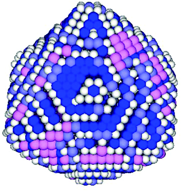Fig. 5 Illustration of the local coordination analysis of the Au nanoparticles. This nanoparticle corresponds to a temperature of 23 °C and an initial [Au⁺]₀ of 12.5 mM. The Au sites are colored according to their classification as: blue (111), pink (100), white (steps/edges), and lavender (indeterminate).

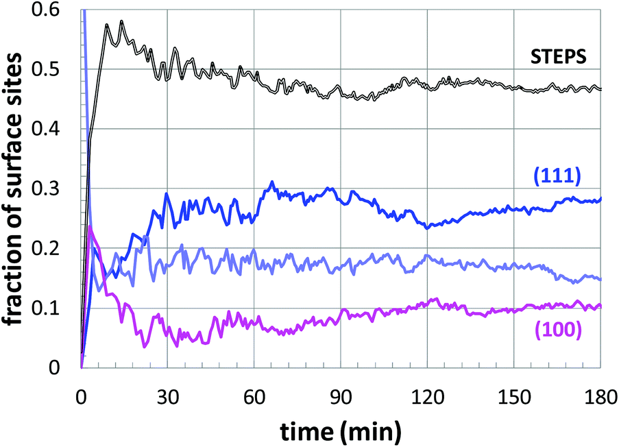Fig. 6 The time evolution of the surface structure of a growing Au nanoparticle, corresponding to a temperature of 23 °C and an initial [Au⁺]₀ of 12.5 mM. The curves correspond to the different classifications (as shown), with lavender indicating indeterminate sites.

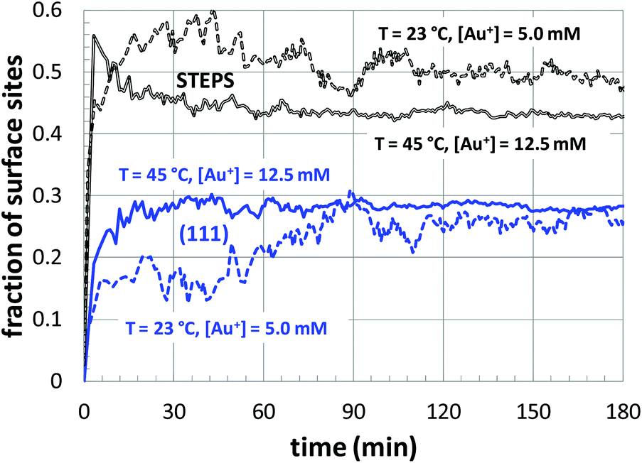Fig. 7 The temporal evolution of the surface sites corresponding to growth conditions of 45 °C and 12.5 mM of [Au⁺]₀versus 23 °C and 5.0 mM of [Au⁺]₀. The colors of the curves are consistent with those of Fig. 6.

3.3 Sensitivity and model analysis

As mentioned earlier, while the parameter optimization is stable and converges to reasonable values, it is unlikely that the values are truly unique. In lieu of obtaining the exact underlying mechanism and a wide range of experimental benchmarks, this uncertainty will always remain. However, our KMC simulations serve as an excellent test-bed for making progress towards a robust and predictive nanoparticle growth model, especially as more comparisons are made with experiments. At this point, we can gage the sensitivity of the growth predictions with respect to uncertainty in the kinetic rate parameters. Thus, a sensitivity analysis was performed by changing the rate constants in the model (k_ads and k_red) by ±20% and comparing the resulting growth curves to the curve corresponding to the default parameters.

From the results in Fig. 8, it is apparent that there is some flexibility in the parameter fitting. For instance, in Fig. 8(c) a change of k_ads −20% and k_red +20% leads to very similar growth behavior. While this reveals some of the uncertainty in these parameters, the optimization is aided by the availability of multiple sets of experimental growth curves. The different conditions (temperature and initial Au⁺ precursor concentration) allow for a more methodical optimization, such that the rate constants should follow Arrhenius-like behavior as a function of temperature and there should be some consistency maintained when different precursor concentrations are used. This added some soft constraints to the optimization, and future comparisons at other conditions are expected to provide additional value to the fitting procedure.

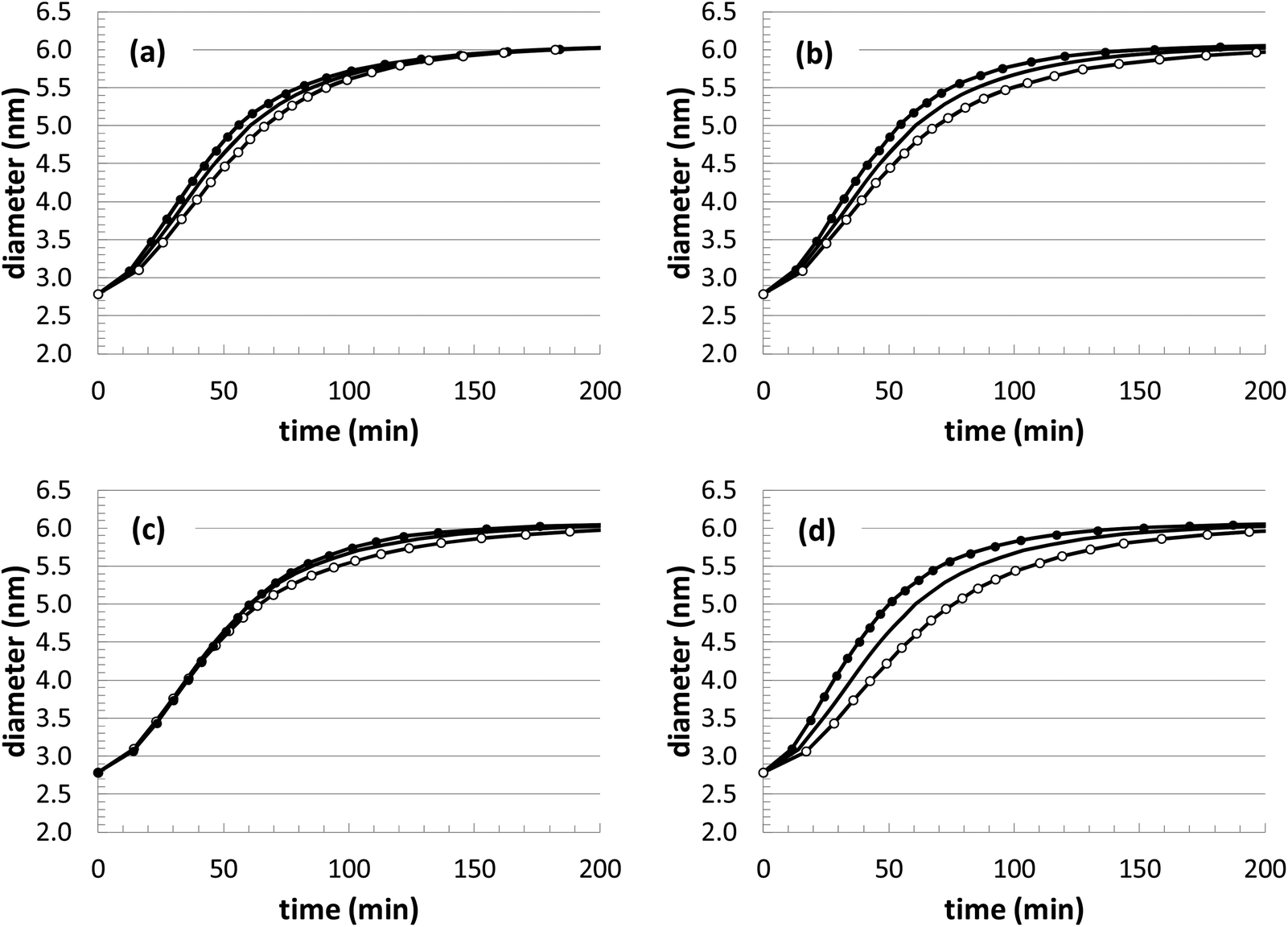Fig. 8 Deviations in the simulated Au nanoparticle growth behavior with respect to variations in the kinetic parameters. The solid black line represents the default parameters. (a) k_ads = ±20% (filled circles/hollow circles); (b) k_red = ±20% (filled circles/hollow circles); (c) k_ads = −20% and k_red = +20% (filled circles), k_ads = +20% and k_red = −20% (hollow circles); (d) k_ads = +20% and k_red = +20% (filled circles), k_ads = −20% and k_red = −20% (hollow circles).

Since there is obviously some flexibility in the parameter fitting, it is important to evaluate the impact on the predicted structural properties. Thus, the surface structure was evaluated when an essentially interchangeable parameter set is used: k_ads = −20% and k_red = +20%, as shown in Fig. 8(c). The structural comparison is shown in Fig. 9, which includes results using the original fitting and using the alternate parameter set. Although there is some inherent uncertainty in the data, the results are very similar (and distinct from the other growth conditions), indicating that moderate uncertainty in the parameter fitting should still yield consistent structural predictions.

Fig. 9 Comparison of nanoparticle surface structure predictions: (solid lines) fitted parameters (Table 2); and (dashed lines) perturbed parameters of k_ads = −20% and k_red = +20% (corresponding to the filled circles in Fig. 8(c)).

With any modeling approach, it is valuable to be able to make predictions at unknown conditions. In our model, the thermal behavior seems to be accurately captured. For instance, we can use the parameter fits at the two lowest temperatures to make a prediction at the highest temperature by assuming Arrhenius-type scaling behavior. Results from the optimized parameter set (Table 2) and the predicted parameter set are show in Fig. 10(a), and the comparison is excellent. However, if we attempt the same comparison with respect to changes in the initial precursor concentration, there are large deviations observed (Fig. 10(b)). In this comparison, we simply assume that the underlying rate constants should not be significantly affected by the different initial precursor concentrations. Thus, we use the average parameter values at the highest three concentrations to predict the growth at the lowest concentration.

Fig. 10 Estimated growth curves based on model parameter values predicted from other growth conditions. (a) T = 45 °C, [Au⁺]₀ = 12.5 mM; and (b) T = 23 °C, [Au⁺]₀ = 5.0 mM.

While the discrepancy is unfortunate, it raises several important issues. First, the experimental growth behavior at the lowest two concentrations displays some anomalous features. There is a noticeable dip in the growth curve corresponding to the lowest concentration ([Au⁺]₀ = 5.0 mM), and the two lowest concentration growth curves merge after approximately 250 min. Along with this behavior, these two growth conditions also have particularly high polydispersity in the experiments. Thus, it is possible that there are some deviations in the growth mechanism that are occurring at the lower concentrations. For instance, there could be deviations in the relative amount of precursors that are feeding nanoparticle growth versus leading to the nucleation of new nanoparticles. However, without further experimental investigation, the underlying cause for the behavior is unknown.

These initial sensitivity tests indicate that some of the free parameter fitting may be reduced, especially with respect to the behavior at the different temperatures. In terms of the growth at the different initial precursor concentrations, the parameters are almost identical at the highest concentrations, but then deviate by up to 40% at the lower concentrations. If more information about the behavior at the lower two concentrations can be obtained, it may be possible to incorporate additional events in the KMC database, providing more robust predictions with a minimal amount of parameter fitting.

A sensitivity analysis to the value of E_a,diff has also been explored, since there is definitely some uncertainty in the exact value of this parameter. We have probed values of 35 ± 10 kcal mol⁻¹. As expected, there is no difference in the predicted growth curves (since the growth is primarily controlled by k_ads and k_red). With respect to the structure, lower values of E_a,diff tend to reduce scatter in the data (surface features can more easily relax), while larger values increase scatter in the data (enabling longer-lived defect structures). More specifically, values from 30–40 kcal mol⁻¹ result in standard deviations of ±10%, while values nearing 45 kcal mol⁻¹ and above can yield standard deviations of almost 50%. Values lower than 30 kcal mol⁻¹ do not have much additional influence on the surface features, as the diffusion rates become so large that almost all of the moves are diffusion events. The surface atoms just fluctuate among different (yet essentially identical) surface structures, as additional atoms attach to the surface.

Our default value of 35 kcal mol⁻¹ was judged to be a reasonable estimate based on other known values in the literature, and this specific value also demonstrated a good tradeoff in the predicted structural relaxation. In other words, the surfaces are never able to completely relax, but at the same time, significant structural defects are not artificially preserved.

4. Summary

In this work, we have adopted a KMC simulation approach for modeling the atomistic growth behavior of Au nanoparticles. The advantage of our approach is that, compared to traditional MD simulations or DFT calculations, we can track the atomistic nanoparticle structural evolution on time scales that approach the actual experiments. This has allowed us to perform several different comparisons against experimental benchmarks, and it has helped transition our KMC simulations from a hypothetical toy model into a more experimentally-relevant test-bed. In addition, while previous theoretical models have been used for predicting nanoparticle growth, the KMC approach can track atomistic-scale details and account for neighbor–neighbor interactions, structural defects, and structural heterogeneity. These aspects can be particularly influential during nanoparticle growth, leading to a wide variety of interesting nanoparticle geometries.

Our KMC model was refined by performing a series of automated comparisons of Au nanoparticle growth curves versus the experimental observations at different temperatures and initial [Au⁺]₀ seed concentrations. The fitting procedure results in reasonable parameter values, including activation energy barriers that are consistent with related experimental measurements. While the nanoparticle formation mechanism in the KMC simulations is simple, there are opportunities for adding more steps in the future and for testing against different experimental conditions.

Since our KMC simulations preserve the atomistic details of our growing Au nanoparticle, this allows for detailed structural analyses. Although our nanoparticles are roughly spherical, the maximum/minimum dimensions deviate from the average by approximately 12.5%, which is consistent with the corresponding experiments. Also, our surface texture analysis highlights the changes in the surface structure as a function of time. While the nanoparticles show similar surface structures throughout the growth process, there can be some significant differences during the initial growth at different synthesis conditions. In the future, we intend to perform additional benchmarking of more atomistic growth features, including an extension of our model to capture anisotropic nanoparticle growth.

Acknowledgements

CHT an YL acknowledge partial financial support from the National Science Foundation (CBET-1510485, CBET-1511820) and a UA System Collaboration Grant, and CHT acknowledges support from the National Science Foundation (CMMI-1229049).

References

1. A. S. K. Hashmi and G. J. Hutchings, Gold catalysis, Angew. Chem., Int. Ed., 2006, 45, 7896–7936.
2. K. L. Kelly, E. Coronado, L. L. Zhao and G. C. Schatz, The optical properties of metal nanoparticles: The influence of size, shape, and dielectric environment, J. Phys. Chem. B, 2003, 107, 668–677.
3. M. Turner, V. B. Golovko, O. P. H. Vaughan, P. Abdulkin, A. Berenguer-Murcia, M. S. Tikhov, B. F. G. Johnson and R. M. Lambert, Selective oxidation with dioxygen by gold nanoparticle catalysts derived from 55-atom clusters, Nature, 2008, 454, 981–U931.
4. M. Haruta, Gold as a novel catalyst in the 21st century: Preparation, working mechanism and applications, Gold Bull., 2004, 37, 27–36.
5. M. Haruta and M. Date, Advances in the catalysis of Au nanoparticles, Appl. Catal., A, 2001, 222, 427–437.
6. M. Haruta, B. S. Uphade, S. Tsubota and A. Miyamoto, Selective oxidation of propylene over gold deposited on titanium-based oxides, Res. Chem. Intermed., 1998, 24, 329–336.
7. Y. P. Bao, H. Calderon and K. M. Krishnan, Synthesis and characterization of magnetic-optical Co-Au core–shell nanoparticles, J. Phys. Chem. C, 2007, 111, 1941–1944.
8. Y. P. Bao, T. L. Wen, A. C. S. Samia, A. Khandhar and K. M. Krishnan, Magnetic nanoparticles: material engineering and emerging applications in lithography and biomedicine, J. Mater. Sci., 2016, 51, 513–553.
9. D. C. Baiu, C. S. Brazel, Y. P. Bao and M. Otto, Interactions of Iron Oxide Nanoparticles with the Immune System: Challenges and Opportunities for their Use in Nano-oncology, Curr. Pharm. Des., 2013, 19, 6606–6621.
10. P. K. Jain, K. S. Lee, I. H. El-Sayed and M. A. El-Sayed, Calculated absorption and scattering properties of gold nanoparticles of different size, shape, and composition: Applications in biological imaging and biomedicine, J. Phys. Chem. B, 2006, 110, 7238–7248.
11. E. C. Dreaden, A. M. Alkilany, X. Huang, C. J. Murphy and M. A. El-Sayed, The golden age: gold nanoparticles for biomedicine, Chem. Soc. Rev., 2012, 41, 2740–2779.
12. N. D. Burrows, A. M. Vartanian, N. S. Abadeer, E. M. Grzincic, L. M. Jacob, W. Lin, J. Li, J. M. Dennison, J. G. Hinman and C. J. Murphy, Anisotropic nanoparticles and anisotropic surface chemistry, J. Phys. Chem. Lett., 2016, 7, 632–641.
13. N. Thao and H. Yang, Toward Ending the Guessing Game: Study of the Formation of Nanostructures Using In Situ Liquid Transmission Electron Microscopy, J. Phys. Chem. Lett., 2015, 6, 5051–5061.
14. X. Chen, J. Schroeder, S. Hauschild, S. Rosenfeldt, M. Dulle and S. Foerster, Simultaneous SAXS/WAXS/UV-Vis Study of the Nucleation and Growth of Nanoparticles: A Test of Classical Nucleation Theory, Langmuir, 2015, 31, 11678–11691.
15. G. Grochola, S. P. Russo and I. K. Snook, On the formation mechanism of the “pancake” decahedron gold nanoparticle, J. Chem. Phys., 2007, 127, 224705.
16. A. Loubat, L.-M. Lacroix, A. Robert, M. Imperor-Clerc, R. Poteau, L. Maron, R. Arenal, B. Pansu and G. Viau, Ultrathin Gold Nanowires: Soft-Templating versus Liquid Phase Synthesis, a Quantitative Study, J. Phys. Chem. C, 2015, 119, 4422–4430.
17. G. Mpourmpakis, S. Caratzoulas and D. G. Vlachos, What Controls Au Nanoparticle Dispersity during Growth?, Nano Lett., 2010, 10, 3408–3413.
18. D. V. Talapin, A. L. Rogach, M. Haase and H. Weller, Evolution of an ensemble of nanoparticles in a colloidal solution: Theoretical study, J. Phys. Chem. B, 2001, 105, 12278–12285.
19. M. A. El-Sayed, Some interesting properties of metals confined in time and nanometer space of different shapes, Acc. Chem. Res., 2001, 34, 257–264.
20. C. J. Murphy, A. M. Gole, J. W. Stone, P. N. Sisco, A. M. Alkilany, E. C. Goldsmith and S. C. Baxter, Gold Nanoparticles in Biology: Beyond Toxicity to Cellular Imaging, Acc. Chem. Res., 2008, 41, 1721–1730.
21. C. Y. Liu, Y. Pei, H. Sun and J. Ma, The Nucleation and Growth Mechanism of Thiolate-Protected Au Nanoclusters, J. Am. Chem. Soc., 2015, 137, 15809–15816.
22. S. M. Neidhart, B. M. Barngrover and C. M. Aikens, Theoretical examination of solvent and R group dependence in gold thiolate nanoparticle synthesis, Phys. Chem. Chem. Phys., 2015, 17, 7676–7680.
23. B. M. Barngrover, T. J. Manges and C. M. Aikens, Prediction of Nonradical Au0-Containing Precursors in Nanoparticle Growth Processes, J. Phys. Chem. A, 2015, 119, 889–895.
24. D. E. Jiang, M. L. Tiago, W. D. Luo and S. Dai, The “Staple” motif: A key to stability of thiolate-protected gold nanoclusters, J. Am. Chem. Soc., 2008, 130, 2777–2779.
25. L. Xiao, B. Tollberg, X. K. Hu and L. C. Wang, Structural study of gold clusters, J. Chem. Phys., 2006, 124, 114309.
26. R. G. Shimmin, A. B. Schoch and P. V. Braun, Polymer size and concentration effects on the size of gold nanoparticles capped by polymeric thiols, Langmuir, 2004, 20, 5613–5620.
27. B. Abecassis, F. Testard, Q. Y. Kong, B. Francois and O. Spalla, Influence of Monomer Feeding on a Fast Cold Nanoparticles Synthesis: Time-Resolved XANES and SAXS Experiments, Langmuir, 2010, 26, 13847–13854.
28. A. Henkel, O. Schubert, A. Plech and C. Sonnichsen, Growth Kinetic of a Rod-Shaped Metal Nanocrystal, J. Phys. Chem. C, 2009, 113, 10390–10394.
29. S. R. K. Perala and S. Kumar, On the Mechanism of Metal Nanoparticle Synthesis in the Brust-Schiffrin Method, Langmuir, 2013, 29, 9863–9873.
30. P. J. Skrdla, Use of Dispersive Kinetic Models for Nucleation and Denucleation to Predict Steady-State Nanoparticle Size Distributions and the Role of Ostwald Ripening, J. Phys. Chem. C, 2012, 116, 214–225.
31. A. Bruma, U. Santiago, D. Alducin, G. Plascencia Villa, R. L. Whetten, A. Ponce, M. Mariscal and M. José-Yacamán, Structure Determination of Superatom Metallic Clusters Using Rapid Scanning Electron Diffraction, J. Phys. Chem. C, 2016, 120, 1902–1908.
32. D. F. Mukhamedzyanova, N. K. Ratmanova, D. A. Pichugina and N. E. Kuz'menko, A Structural and Stability Evaluation of Au-12 from an Isolated Cluster to the Deposited Material, J. Phys. Chem. C, 2012, 116, 11507–11518.
33. D. J. Earl and M. W. Deem, Parallel tempering: Theory, applications, and new perspectives, Phys. Chem. Chem. Phys., 2005, 7, 3910–3916.
34. G. M. Torrie and J. P. Valleau, Non-physical sampling distributions in Monte-Carlo free-energy estimation - umbrella sampling, J. Comput. Phys., 1977, 23, 187–199.
35. A. Laio and F. L. Gervasio, Metadynamics: a method to simulate rare events and reconstruct the free energy in biophysics, chemistry and material science, Rep. Prog. Phys., 2008, 71, 126601.
36. A. Laio and M. Parrinello, Escaping free-energy minima, Proc. Natl. Acad. Sci. U. S. A., 2002, 99, 12562–12566.
37. L. Pavan, K. Rossi and F. Baletto, Metallic nanoparticles meet metadynamics, J. Chem. Phys., 2015, 143, 184304.
38. F. Baletto, C. Mottet, A. Rapallo, G. Rossi and R. Ferrando, Growth and energetic stability of AgNi core-shell clusters, Surf. Sci., 2004, 566, 192–196.
39. A. B. Bortz, M. H. Kalos and J. L. Lebowitz, New algorithm for Monte-Carlo simulation of Ising systems, J. Comput. Phys., 1975, 17, 10–18.
40. D. P. Landau and K. Binder, A Guide to Monte Carlo Simulations in Statistical Physics, Cambridge, United Kingdom, 2005.
41. D. T. Gillespie, General method for numerically simulating stochastic time evolution of coupled chemical-reactions, J. Comput. Phys., 1976, 22, 403–434.
42. A. F. Voter, Classically exact overlayer dynamics - diffusion of rhodium clusters on Rh100, Phys. Rev. B: Condens. Matter, 1986, 34, 6819–6829.
43. K. A. Fichthorn and W. H. Weinberg, Theoretical foundations of dynamic Monte-Carlo simulations, J. Chem. Phys., 1991, 95, 1090–1096.
44. S. Piana, M. Reyhani and J. D. Gale, Simulating micrometre-scale crystal growth from solution, Nature, 2005, 438, 70–73.
45. R. Theissmann, M. Fendrich, R. Zinetullin, G. Guenther, G. Schierning and D. E. Wolf, Crystallographic reorientation and nanoparticle coalescence, Phys. Rev. B: Condens. Matter, 2008, 78, 205413.
46. X. Wang, K. C. Lau, C. H. Turner and B. I. Dunlap, Kinetic Monte Carlo simulation of the elementary electrochemistry in a hydrogen-powered solid oxide fuel cell, J. Power Sources, 2010, 195, 4177–4184.
47. K. C. Lau, C. H. Turner and B. I. Dunlap, Kinetic Monte Carlo simulation of O2- incorporation in the yttria stabilized zirconia YSZ fuel cell, Chem. Phys. Lett., 2009, 471, 326–330.
48. K. C. Lau, C. H. Turner and B. I. Dunlap, Kinetic Monte Carlo simulation of the Yttria Stabilized Zirconia YSZ fuel cell cathode, Solid State Ionics, 2008, 179, 1912–1920.
49. R. Pornprasertsuk, J. Cheng, H. Huang and F. B. Prinz, Electrochemical impedance analysis of solid oxide fuel cell electrolyte using kinetic Monte Carlo technique, Solid State Ionics, 2007, 178, 195–205.
50. R. Pornprasertsuk, P. Ramanarayanan, C. B. Musgrave and F. B. Prinz, Predicting ionic conductivity of solid oxide fuel cell electrolyte from first principles, J. Appl. Phys., 2005, 98, 103513.
51. L. G. Wang and P. Clancy, Kinetic Monte Carlo simulation of the growth of polycrystalline Cu films, Surf. Sci., 2001, 473, 25–38.
52. J. G. Amar and F. Family, Effects of crystalline microstructure on epitaxial growth, Phys. Rev. B: Condens. Matter, 1996, 54, 14742–14753.
53. C. C. Battaile, D. J. Srolovitz and J. E. Butler, A kinetic Monte Carlo method for the atomic-scale simulation of chemical vapor deposition: Application to diamond, J. Appl. Phys., 1997, 82, 6293–6300.
54. H. N. G. Wadley, A. X. Zhou, R. A. Johnson and M. Neurock, Mechanisms, models and methods of vapor deposition, Prog. Mater. Sci., 2001, 46, 329–377.
55. H. Jiang and Z. Hou, Large-scale epitaxial growth kinetics of graphene: A kinetic Monte Carlo study, J. Chem. Phys., 2015, 143, 084109.
56. W. J. Rodgers, P. W. May, N. L. Allan and J. N. Harvey, Three-dimensional kinetic Monte Carlo simulations of diamond chemical vapor deposition, J. Chem. Phys., 2015, 142, 214707.
57. D. Mei, J. Du and M. Neurock, First-Principles-Based Kinetic Monte Carlo Simulation of Nitric Oxide Reduction over Platinum Nanoparticles under Lean-Burn Conditions, Ind. Eng. Chem. Res., 2010, 49, 10364–10373.
58. D. Mei, P. A. Sheth, M. Neurock and C. M. Smith, First-principles-based kinetic Monte Carlo simulation of the selective hydrogenation of acetylene over Pd111, J. Catal., 2006, 242, 1–15.
59. L. D. Kieken, M. Neurock and D. H. Mei, Screening by kinetic Monte Carlo simulation of Pt-Au100 surfaces for the steady-state decomposition of nitric oxide in excess dioxygen, J. Phys. Chem. B, 2005, 109, 2234–2244.
60. E. W. Hansen and M. Neurock, First-principles-based Monte Carlo simulation of ethylene hydrogenation kinetics on Pd, J. Catal., 2000, 196, 241–252.
61. E. Martinez, J. Marian, M. H. Kalos and J. M. Perlado, Synchronous parallel kinetic Monte Carlo for continuum diffusion-reaction systems, J. Comput. Phys., 2008, 227, 3804–3823.
62. P. Haldar and A. Chatterjee, Seeking kinetic pathways relevant to the structural evolution of metal nanoparticles, Modell. Simul. Mater. Sci. Eng., 2015, 23, 025002.
63. M. R. Sorensen and A. F. Voter, Temperature-accelerated dynamics for simulation of infrequent events, J. Chem. Phys., 2000, 112, 9599–9606.
64. V. Gorshkov, V. Kuzmenko and V. Privman, Modeling of Growth Morphology of Core-Shell Nanoparticles, J. Phys. Chem. C, 2014, 118, 24959–24966.
65. V. Gorshkov, A. Zavalov and V. Privman, Shape Selection in Diffusive Growth of Colloids and Nanoparticles, Langmuir, 2009, 25, 7940–7953.
66. E. Elkoraychy, K. Sbiaai, M. Mazroui, Y. Boughaleb and R. Ferrando, Numerical study of hetero-adsorption and diffusion on 100 and 110 surfaces of Cu, Ag and Au, Surf. Sci., 2015, 635, 64–69.
67. S. M. Foiles, M. I. Baskes and M. S. Daw, Embedded-atom-method functions for the FCC metals Cu, Ag, Au, Ni, Pd, Pt, and their alloys, Phys. Rev. B: Condens. Matter, 1986, 33, 7983–7991.
68. M. R. LaBrosse, J. K. Johnson and A. C. T. van Duin, Development of a Transferable Reactive Force Field for Cobalt, J. Phys. Chem. A, 2010, 114, 5855–5861.
69. C. L. Liu, J. M. Cohen, J. B. Adams and A. F. Voter, EAM study of surface self-diffusion of single adatoms of FCC metals Ni, Cu, Al, Ag, Au, Pd, and Pt, Surf. Sci., 1991, 253, 334–344.
70. C. H. Claassens, J. J. Terblans, M. J. H. Hoffman and H. C. Swart, Kinetic Monte Carlo simulation of monolayer gold film growth on a graphite substrate, Surf. Interface Anal., 2005, 37, 1021–1026.
71. L. G. Wang and P. Clancy, Kinetic Monte Carlo simulation of the growth of polycrystalline Cu films, Surf. Sci., 2001, 473, 25–38.
72. F. Li, H. Zhang, B. Dever, X.-F. Li and X. C. Le, Thermal Stability of DNA Functionalized Gold Nanoparticles, Bioconjugate Chem., 2013, 24, 1790–1797.
73. B. Abecassis, F. Testard, O. Spalla and P. Barboux, Probing in situ the nucleation and growth of gold nanoparticles by small-angle x-ray scattering, Nano Lett., 2007, 7, 1723–1727.
74. M. Wojnicki, E. Rudnik, M. Luty-Blocho, K. Paclawski and K. Fitzner, Kinetic studies of gold(III) chloride complex reduction and solid phase precipitation in acidic aqueous system using dimethylamine borane as reducing agent, Hydrometallurgy, 2012, 127, 43–53.
75. K. Paclawski and K. Fitzner, Kinetics of gold(III) chloride complex reduction using sulfurIV, Metall. Mater. Trans. B, 2004, 35, 1071–1085.

---