Interfacing digital microfluidics with high-field nuclear magnetic resonance spectroscopy

Abstract

Nuclear magnetic resonance (NMR) spectroscopy is extremely powerful for chemical analysis but it suffers from lower mass sensitivity compared to many other analytical detection methods. NMR microcoils have been developed in response to this limitation, but interfacing these coils with small sample volumes is a challenge. We introduce here the first digital microfluidic system capable of interfacing droplets of analyte with microcoils in a high-field NMR spectrometer. A finite element simulation was performed to assist in determining appropriate system parameters. After optimization, droplets inside the spectrometer could be controlled remotely, permitting the observation of processes such as xylose–borate complexation and glucose oxidase catalysis. We propose that the combination of DMF and NMR will be a useful new tool for a wide range of applications in chemical analysis.

---

Introduction

Nuclear magnetic resonance (NMR) spectroscopy is a non-destructive analytical technique that allows the user to probe the chemical environment of nuclei that have non-zero spin (including ¹H and ¹³C, among others). NMR is thus capable of providing more information about chemical structure than can be found when using many other analysis techniques. This has made NMR a popular tool for studying environmental contaminants,¹ protein conformation dynamics,² diffusion kinetics,³ and many other applications.

A key limitation of NMR is its low mass sensitivity,⁴ a disadvantage for applications involving analytes present at low concentrations or for those involving compounds that are difficult or expensive to synthesize. Several strategies have been developed to address this challenge, the most common being the use of increased static magnetic field strengths (which generates a larger population of spins aligned with the field); this has led to the trend of ever-increasing sizes and costs of cutting-edge NMR spectrometers. A second strategy to solve low mass sensitivities in NMR is hyperpolarization, a technique in which the nuclear spin polarization state is brought to a level far higher than the equilibrium value, prior to analysis. For example, dynamic nuclear polarization⁵ (DNP) is now a common technique in NMR imaging, useful for studying metabolic flux in complex biological samples (e.g., perfused model-organ systems⁶). Finally, a third strategy is to reduce the size of the receiver coil, which has led to the development of so-called microcoils (i.e., coils with sub-mm diameters). This approach leverages the fact that the magnetic flux density induced by a unit current (and therefore the voltage induced in the coil by nuclear spins) increases at a greater rate than the resistive noise, leading to improved signal-to-noise ratios.^7,8

The growing interest in the use of microcoils for NMR spectroscopy has triggered a related movement to develop micro-volume systems that can position samples of interest near the coil and ensure appropriate filling factors.⁹ A number of groups have described innovative microchannel/microcoil NMR systems employing solenoid microcoils,^10–12 planar microcoils,^13–18 microstriplines,¹⁹ and microslots²⁰ that have proven useful for a variety of applications. But the most common paradigm of enclosed microchannels with continuous flow has two limitations for combination with NMR spectroscopy. First, while microcoils have small detection volumes (i.e., the volume of solution adjacent to the microcoil), most microchannel-based systems suffer from large dead volumes associated with the pumps and tubing used to flow the samples through the channels (note that when microcoils are used to study solids^21,22 they are immune from this issue). Second, if one wishes to study time-resolved reaction phenomena in microchannels, it is necessary to continuously flow reagents through the system, which results in increased reagent use. For example, one study which employed solenoid microcoils¹² evaluated protein unfolding dynamics after reaction-times ranging from 3.8 s to 114 s, by varying the flow rate from 60 μL min⁻¹ to 2 μL min⁻¹, respectively. This increased reagent use is exacerbated by the fact that microcoils often have detection volumes in range of microliters; thus, depending on kinetics and acquisition parameters, microfluidic systems can require the use of hundreds to thousands of microliters of sample per experiment. A second paradigm for microscale NMR uses plugs or droplets within channels or tubes to study reactions. For example, Kautz et al.¹¹ interfaced a droplet microfluidic system with a custom solenoid microcoil and highlighted the promise of the technique in an automated analysis of a library of compounds for pharmaceutical research. The advantage of this system is the elimination of dead volume issues found in continuous-flow microfluidics. Further, one could potentially use this type of system to de-couple reaction time from flow; however, the initiation of reactions inside the spectrometer for this type of system has not been demonstrated, and precise positioning of sample droplets relative to the microcoil is challenging.¹⁰ There is thus a need for a new technique that allows for complete user-control over micro-scale volumes of reagents and analytes in microcoil-NMR spectroscopy.

Digital microfluidics (DMF) is a third microfluidic paradigm which may be able to fill the need described above. In digital microfluidics, droplets of fluid are precisely manipulated on an insulated, hydrophobic electrode array by applying appropriate voltages to sequences of electrodes in the array.²³ DMF has previously been interfaced with analytical techniques such as mass spectrometry,²⁴ electrochemistry,²⁵ and immunoassays.²⁶ Very recently, Lei et al.^27,28 reported the first interface between DMF and magnetic resonance using planar microcoils. In this work, a low-field (0.46 T) magnetic relaxometer was used to detect changes in the T2 relaxation of water droplets as iron particles distributed therein became aggregated. This system represents an exciting step forward for portable NMR analysis, but the weak magnetic field makes it inappropriate for conventional NMR spectroscopy of chemical analytes.

Here we report the first system interfacing digital microfluidics with high-field NMR spectroscopy, appropriate for chemical characterization (i.e. identification of chemical shifts and chemical shift changes associated with reactions). DMF devices were developed to interface with a 920 μm outer-diameter planar microcoil, such that discrete μL-volume droplets could be manipulated onto and off of the coil surface, permitting the observation of processes such as xylose–borate complexation and glucose oxidase catalysis. We propose that this work represents an important first step for using DMF to characterize reaction dynamics with NMR, as well as breaking new ground for applications combining digital microfluidics with high magnetic fields.

Theory and simulations

When nuclei are placed in an external magnetic field, their magnetic moments precess about the direction of the field at a frequency that is proportional to the magnitude of the field. This is known as Larmor precession and its frequency ω is given by eqn (1),

ω = γB (1)

where γ is the gyromagnetic ratio of the nuclei, B is the flux density of the external magnetic field, and the direction of precession is given by the right-hand rule. A critical goal in NMR spectrometer design is to ensure that all chemically equivalent nuclei precess at the same frequency regardless of where they are found within the sample volume. The degree to which this is accomplished determines the ultimate resolution of the spectra. Achieving uniform precession frequency requires a uniform magnetic flux density, which is in turn controlled by the uniformity of the magnetic field. Thus, the most expensive (and most carefully designed) part of an NMR spectrometer is the superconducting coil assembly that surrounds the sample used to generate the static magnetic field.

The initial magnetic flux density is altered as the magnetic moments of the sample align to the applied field to either enhance or reduce the original flux density. This is formally expressed in the constitutive relation (2) which gives the static field B₀,

B₀ = μ₀(H + M) (2)

where μ₀ is the permeability of vacuum with a value of 4π × 10⁻⁷ H m⁻¹, H is the applied magnetic field, and M is the magnetization vector. Depending on the geometry and composition of the sample and surroundings, the contribution from sample magnetization can cause the magnetic flux density to vary significantly within the sample volume. For magnetically linear materials, the induced magnetization vector has a relatively simple form (3),

M = χ_iH (3)

where χ_i is the magnetic susceptibility of diamagnetic material i. In this work the materials of interest are air (χ_air = 3.6 × 10⁻⁷), water (χ_H2O = −9.0 × 10⁻⁶), silicon dioxide (χ_SiO2 = −1.6 × 10⁻⁶), and copper (χ_Cu = −9.6 × 10⁻⁶). The susceptibility difference between air and water (at the edge of a droplet on a device) is one cause of varying magnetic flux (and therefore non-uniform Larmor frequencies) within the sample volume.

To approximate magnetic flux intensity variations in droplets on a DMF device, we note that in the sample volume the magnetic field H is given by the following form of Ampère's law (as there is no external current flowing in this region).

∇ × H = 0 (4)

Therefore, the field is conservative in this volume, and can be expressed in terms of the gradient of a scalar magnetic potential V_m. Thus, recognizing the fact that the magnetic flux density has zero divergence, eqn (2) can be rewritten as eqn (5).

−∇·(μ₀∇V_m + μ₀M) = 0 (5)

Eqn (5) was used here to simulate B₀ within droplets in digital microfluidic devices. Corrections for the Lorenz cavity field^29,30 were not included in this model; in the future they might be added for greater accuracy.

To get a complete picture of how the induced magnetization will affect the signal from the spins of interest it is necessary to also have information on the magnetic flux density produced by the microcoil, known as the B₁ field. The electromotive force (emf) generated within the microcoil after the excitation pulse by a particular spin is proportional to the magnitude of the magnetic flux density generated by the coil at that spin's location. The B₁ field generated by a particular microcoil geometry carrying an applied current density J_e can be solved using the general form of Ampère's Law.

∇ × H = J_e (6)

We used 3D COMSOL Multiphysics (COMSOL Inc., Burlington, MA, accessed via license obtained through CMC microsystems, Kingston, ON), using the “magnetic fields, no current” module to solve for the B₀ field expected from eqn (5). Cylindrical droplet geometries were used with the ends of the cylinder having a radius of curvature, R, approximated using eqn (7),³¹

where h = 450 μm is the distance between the DMF device and microcoil surface and θ = 110° is the contact angle of water on a Teflon-AF coated device surface. To simplify the simulation, the device coatings (i.e., the 0.7–3 μm thick dielectric plus ∼0.1 μm thick Teflon-AF) were not included, such that the droplet was sandwiched between two glass surfaces, where the distance between the two surfaces was 450 μm. The size of the domain was reduced by simulating half of a droplet (recognizing the symmetry along the vertical axis); thus, the domain measured 5 × 5 × 10 mm. To simulate the magnetic field of a 500 MHz spectrometer, an 11.74 T magnetic flux density was applied to the bottom boundary and a zero magnetic scalar potential was specified at the top boundary. The remaining boundaries were given the magnetic insulation boundary condition. The droplet domain employed a free tetrahedral mesh with a minimum element size of 0.0002 mm, a maximum element size of 0.005 mm, an element growth rate of 1.1, a resolution of curvature of 0.1, and a resolution of narrow regions of 1. The remaining domains also employed a free tetrahedral mesh but the maximum element size was 0.4 mm, the minimum element size was 0.0001 mm, and the maximum growth rate was 1.07.

The COMSOL Multiphysics “magnetic fields” module was used to calculate the B₁ field (according to eqn 6) produced by a microcoil designed to approximate that of the experimental setup. That is, the coil is located 23 μm below the droplet, has an outer diameter of 920 μm, with 4 turns and 30 μm spacing between turns, and has a wire height and width of 20 μm and 30 μm, respectively. An external current density of 1 A mm⁻² was applied to each coil domain and all exterior boundaries were given the magnetic insulation boundary condition. The resulting fields from both simulations were then exported to generate histograms of the magnetic flux density variation within the droplet using custom Python routines. To calculate the weighted signal, each element was scaled according to the element's size and the magnitude of the B₁ field generated by the microcoil at that element from the “magnetic fields” module. This information was then used to scale the histogram of the magnetic flux density from the “magnetic fields, no current” module.

Experimental

Materials and reagents

Unless otherwise indicated, reagents were purchased from Sigma-Aldrich (Oakville, ON). Glass slides coated with chromium (100 nm) and AZ1500 photoresist (530 nm) were from Telic Inc. (Santa Clarita, CA). AP7156E Pyralux double-sided copper-clad polyimide films were obtained from DuPont Electronic Materials (Research Triangle Park, NC). Parylene-C was from Specialty Coating Systems (Indianapolis, IN), and Teflon-AF 1600 was from DuPont Canada (Mississauga, ON). Microposit MF-312 developer and S1811 positive photoresist were from Rohm and Haas (Marlborough, MA), AZ 300T stripper was from AZ Electronic Materials (Somerville, NJ), and CR-4 Cr etchant was from Cyantek (Freemont, CA). All solutions used to obtain NMR spectra were prepared in 99.9% deuterium oxide.

NMR spectrometer and microcoil

All NMR experiments were performed on a Bruker Avance III spectrometer operating at the ¹H frequency of 499.98 MHz. The NMR microcoils were fabricated by Bruker Biospin (Billerica, MA and Fällanden Switzerland) and mounted to a PEEK coil-holder that was interfaced to a micro-05 Broadband 2-channel H-X NMR probe (Bruker GMBH, Rheinstetten Germany). The probe was operated with a 90° pulse determined through a nutation curve at 0.1 W, which is within the specifications of the coil. The pulse duration at this power level is ∼5–8 μs depending on sample salinity and composition. See the online ESI† for coil layout, dimensions and nutation experiment.

DMF device fabrication and operation

Masks for DMF device top-plates were printed using a Heidelberg uPG 501 mask writer (Heidelberg Instruments Mikrotechnik GmbH, Germany) in the Center for Microfluidic Systems at the University of Toronto, and the top-plates were fabricated in the Toronto Nanofabrication Centre cleanroom at the University of Toronto. Chromium and photoresist-coated glass substrates were exposed for 10 seconds in a mask aligner and then developed in Microposit MF-312 for 30 seconds. They were then rinsed in water and immersed in CR-4 chromium enchant until the electrode patterns developed. After a final rinse, the devices were dried using nitrogen, and the substrate was diced to yield eight 19 mm × 25 mm devices. Each device featured one of two designs: device A comprises six electrodes in a “line” pattern (five 1.5 mm × 1.5 mm electrodes adjacent to a 7.6 mm × 1.35 mm electrode). Device B features eight electrodes in an “H” pattern [three electrodes on each side of the “H” (one 1.5 mm × 7.5 mm electrode and two 1.5 mm × 3.75 mm electrodes) and two 3 mm × 1.5 mm electrodes in the center of the “H”]. All electrodes were spaced 30 μm from each other, and each was connected to a contact pad on the edge of the substrate.

After forming the electrode patterns, device top-plates were coated with a dielectric layer (either parylene C or silicon nitride). Parylene C films (3 μm) were deposited on device A substrates using a SCS 2010 Parylene Coater (Specialty Coating Systems) using 7 grams of parylene. Silicon nitride films (700 nm) were deposited on device B substrates via plasma enhanced chemical vapor deposition using an Oxford Instruments PlasmaLab System 100 PECVD (Oxford Instruments, UK). After dielectric layer deposition, a hydrophobic layer was applied by spin coating (2000 rpm, 30 s) a 1% w/w solution of Teflon AF in FC-40 and post-baking at 160 °C on a hot-plate for 10 minutes.

Electrical connections were made to the contact pads on DMF top plates using custom manifolds formed by laser printing/etching (using techniques similar to those described previously^32,33). Briefly, each manifold was formed by printing laser toner in a pattern of eight circular electrodes (radius of 0.75 mm) connected to eight square contact pads (1.5 mm × 1.5 mm) onto an AP7156E Pyralux film using a Xerox Phaser 6700 printer (Norwalk, CT). When needed, pinholes in the patterns were filled in by tracing with a permanent marker. The printed sheet was then immersed in a 1 : 2 solution of hydrochloric acid and 3% hydrogen peroxide until the patterns developed. After rinsing and drying, the circular electrodes were soldered to individual leads in a custom ∼4 m-long CAT5 ethernet cable. The other end of the manifold was affixed to the edge of a DMF top-plate (such that the square pads on the manifold made electrical contact with the contact pads on the device) using 3M970312 conductive adhesive (3M, St. Paul, MN).

DMF device top plates (as above) were assembled with a bottom plate bearing an NMR coil (as per below), with droplets sandwiched between the two plates. Droplet position was controlled by applying potentials (260–300 V_RMS, 10 kHz for parylene-coated devices and 140–200 V_RMS, 1 kHz for silicon nitride coated devices) between the driving and counter electrodes on the top plate. The potentials were programmed and managed using the open-source DropBot³⁴ DMF control system via the CAT5 ethernet cable.

DMF–NMR interface and operation

DMF device bottom-plates were formed from a custom Bruker planar microcoil covered by a 10 mm × 10 mm × 10 μm coating of SU-8 photoresist (forming a “working surface”); see the online ESI† for details. A 1 μL droplet of FC-40 oil was deposited on the working surface. A 10 cm × 30 cm × 12.5 μm thick fluorinated ethylene propylene (FEP) film (CS Hyde Company, Lake Villa, IL) was positioned on top of the oil-laden working surface. Excess oil was removed with a Q-Tip and the film was affixed with labeling tape. Immediately prior to use, another 1 μL droplet of FC-40 oil was spread over the surface of the FEP film using a Q-Tip. Droplets of reagents were loaded onto the bottom-plate, and a stack of 8–10 pieces of double-sided tape (3M, St. Paul, MN) were placed on either side of the working surface. The top-plate was then positioned above the bottom-plate (with the coil aligned to the center of the array of DMF driving electrodes) such that the space between the FEP film (on the microcoil assembly) and the Teflon-AF coating (on the DMF top-plate) was approximately 350–450 μm. Labeling tape (Fisher Scientific, Waltham, MA) was wrapped around the integrated DMF device/microcoil assembly; in long-duration experiments, the assembly was also wrapped in Teflon tape (Home Depot, Toronto, ON).

At the start of each DMF–NMR experiment, an integrated device/assembly was loaded into the central bore of the spectrometer so that the DMF device was oriented vertically. Briefly, the integrated device/assembly was pulled up the bore (from bottom to top), and the CAT5 ethernet cable was fed out of the top of the bore to connect with a DropBot.³⁴ In a typical experiment, the sample was shimmed, and 1D ¹H spectra were acquired using an 8 μs 90° pulse and an 8 kHz spectrum window, 16 000 data points, averaging over 16 scans with a recycle delay of 1 second. In some cases, ¹H–¹H total correlation spectroscopy (TOCSY) spectra (generated from standard mixing sequences^35,36) were acquired using phase sensitive (states-tppi) mode, a 5.5 μs 90° pulse, an 8 kHz spectrum window, a TOCSY mixing time of 120 ms, and a 7 KHz spin lock field strength, averaging over 8 scans with a recycle delay of 1 s. In the latter experiments, 16 000 data points were collected for each of the 128 increments in the F1 indirect dimension.

Volume response and droplet movement

Replicates of device A with inter-plate spacing of 350 μm were used to evaluate volume-response by generating spectra from a series of droplets with varying volumes (1.2–10 μL) of 0.1 M sucrose. Replicates of device B with inter-plate spacing of 450 μm were used to evaluate droplet movements. The latter was accomplished by first loading two reagents onto either side of a device: a 5 μL droplet of D₂O and a 5 μL droplet of 0.1 M sucrose. After loading into the spectrometer, each droplet was cycled onto and off of the microcoil, collecting spectra after each operation.

Xylose–borate reaction

Replicates of device A with inter-plate spacing of 450 μm were used to evaluate the xylose–borate reaction. In a series of experiments, two reagents were loaded on either side of a device: a 1.8 μL droplet of 15 mg mL⁻¹ xylose in D₂O and a 1.8 μL droplet of 3 mg mL⁻¹ borate in D₂O. After loading into the instrument, the borate droplet was actuated onto the microcoil and a spectrum was collected. The borate and xylose droplets were then merged and mixed for approximately 1 minute by actuating the droplet back and forth across the device, and a second spectrum was collected. The shimming and data acquisition took sufficient time such that the total time elapsed between spectra was approximately 10 min.

Glucose-oxidase reaction

Replicates of device A with inter-plate spacing of 450 μm were used to evaluate the glucose-oxidase reaction. In a series of experiments, two reagents were loaded onto either side of a device: a 1.8 μL droplet containing 3.2 mg mL⁻¹ glucose oxidase, and a 1.8 μL droplet containing 25 mg mL⁻¹ of glucose and 1.6 mg mL⁻¹ of horse radish peroxidase (HRP). The reaction was initiated by merging the two droplets and actuating them across the array for approximately 1.5 minutes. Upon completion of the mixing procedure the resultant droplet was driven onto the microcoil. The assembly was then loaded into the spectrometer and spectra were collected after 6, 18, 36, or 44 min incubation.

Results and discussion

Interfacing NMR and DMF

NMR spectroscopy with microcoils is becoming increasingly popular, which has necessitated the development of microfluidic tools to deliver samples into the appropriate detection volume. All microfluidic methods reported previously for use with high-field NMR spectroscopy have relied on enclosed microchannels or tubes.^{7,9–16,18–20} Many of these systems have limitations, which include large sample dead volumes and temporal resolution that is based on flow rate and residence time (for continuous format) or an inability to initiate reactions and challenges with analyte positioning (for droplet format). We hypothesized that these limitations might be overcome using digital microfluidics, which allows for precise positioning of droplets with no dead-volume, and allows the user to de-couple reaction-time from flow. While these advantages make the integration of DMF with NMR appealing, there were significant challenges that impeded the integration of the two techniques, including DMF-microcoil limitations, DMF-spectrometer limitations, and magnetic field homogeneity questions. Each of these challenges required significant design innovation/optimization and trial-and-error to overcome, as described below.

The first challenge for integrating DMF and NMR is determining how to interface droplet handling with an NMR microcoil. The Bruker planar microcoil used here (Fig. 1a) is a 920 μm outer-diameter four-turn copper coil buried under a 10 × 10 mm insulating coating (see Fig. S1 and S2 in the online ESI† for details). This geometry poses three key constraints for DMF: working area, droplet manipulation, and microcoil re-use. For the first constraint, the 10 × 10 mm active area is small relative to conventional DMF devices (which often cover several square centimeters of active area). Thus, the DMF devices used here were uncharacteristically small, comprising just six (Fig. 1b) or eight driving electrodes. For the second constraint, the standard “two plate” DMF mode²³ (in which droplets are sandwiched between driving electrodes on one plate and a counter-electrode on the other plate) was not accessible for this technique – one of the “plates” is occupied by the NMR microcoil. Thus, in this work, DMF was operated in single-plate mode,²³ in which droplets are manipulated via electrostatic forces generated by applying potentials between electrodes on the same plate. Finally, for the third constraint: the NMR microcoil was not disposable, which required that it be protected under a removable film (in this case 12.5 μm-thick FEP) that could be replaced after each use (this strategy has been reported previously for single-plate DMF³⁷). The final DMF-microcoil assembly used here (accounting for each of the constraints described above) is shown in Fig. 1c. The distances between the microcoil and DMF device were chosen such that viscous forces were high enough to help keep the droplet in place as it was being loaded into the spectrometer but not so great such that they prevented the droplet from moving. This arrangement was found to be suitable for proof-of-principle, but for future work, we are working to generate custom microcoil assemblies that address the limitations described above.

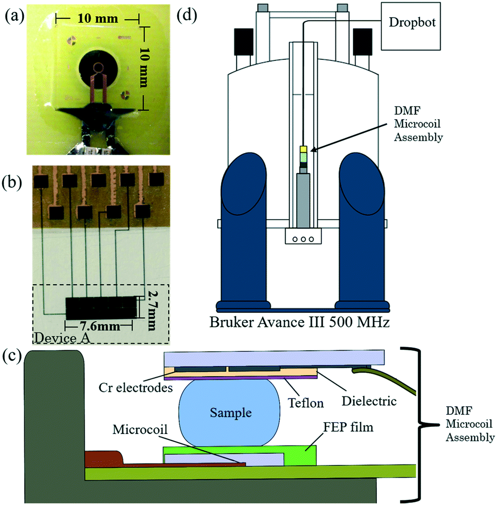Fig. 1 Digital microfluidics for nuclear magnetic resonance spectroscopy (DMF–NMR). (a) Picture of Bruker planar microcoil (outer-diameter 920 μm) used in this work. The working area for droplet actuation is defined by a flat 10 mm × 10 mm coating. (b) Picture of DMF top-plate (device A) showing the electrical contacts (top) and the actuation electrodes (bottom). When an appropriate electric potential is applied between electrodes on the substrate, droplets will move until they are centered between the electrode pair. (c) Schematic of the probe assembly, illustrating how a sample droplet is sandwiched between the DMF device (top) and microcoil (bottom). (d) Schematic showing position of probe and DMF-microcoil in the spectrometer as well as the connection to the Dropbot automation system.

The second challenge for integrating DMF and NMR is determining how to interface the DMF-microcoil assembly with the spectrometer (the instrument used here was a Bruker Avance III 500 MHz system). DMF devices are typically operated horizontally (where gravity is not a force that must be overcome), and in a system that allows for convenient tracking of droplet position by eye or camera. In contrast, in the new system reported here, the device is oriented vertically (inside the bore of the NMR magnet) and is located several meters away from the operator (Fig. 1d). A custom interface/cable was developed to allow for remote actuation (with no visual feedback), and it was determined that actuation electrodes must always be activated during the loading process to prevent gravity-driven droplet loss. The latter (always-on electrodes) reduces device lifetime, as the dielectric layer becomes irreversibly altered after long-term use.³⁸ In addition, device lifetime appears to be limited by other phenomena, perhaps related to the interaction between the applied magnetic field and the device/cabling/interface (a topic of on-going research). In practice, devices were observed to enable reliable droplet movement (with no differences observed between devices bearing dielectric layers formed from silicon nitride or parylene-C) for several minutes within the spectrometer, which was sufficient for the applications described here. In on-going work, new prototypes are being developed that will allow horizontal (and presumably longer-lifetime) device operation.

The third challenge for integrating DMF and NMR is the necessity of using a geometry that minimizes heterogeneities in the magnetic flux density (see the Theory and simulations section for equations and details). To evaluate the magnetic flux inhomogeneity caused by the susceptibility mismatch between the droplet and the surrounding medium (air), eqn (5) was solved using finite-element numerical methods in COMSOL Multiphysics. Fig. 2a shows a three-dimensional representation of a droplet adjacent to the microcoil. When the 11.74 T-magnetic flux density B₀ is applied along the z-axis, the magnetic moments of the molecules in the droplet align, inducing a secondary field that either opposes or enhances B₀. Because water is diamagnetic, the induced secondary field in this case opposes B₀, reducing the magnetic flux density within the droplet. This effect can be quantified in terms of a ratio relative to the applied field, ΔB/B₀, measured in parts per million (ppm). This ratio is plotted as a heat-map for a zy-slice of the system for a 2 μL and a 4 μL droplet in Fig. 2b and c, respectively. As shown, the fields experienced by molecules in the different droplets vary from −3.8 ppm to −7 ppm below the applied field strength of 11.74 T. An alternate view of the system (featuring an xy-slice) is shown in Fig. 2c, with simulations of the flux density variation (as heat maps) in that plane for a 2 μL and a 4 μL droplet in Fig. 2d and e, respectively. As shown, the maximum variation in the different droplets in these dimensions range from −5.9 ppm to −7 ppm below the applied 11.74 T field.

Fig. 2 DMF–NMR – simulations of magnetic field homogeneity. (a) Three-dimensional plot of a 2 μL droplet adjacent to the microcoil, highlighting a zx-cut plane. Simulations of (b) a 2 μL and (c) a 4 μL droplet at the zx plane, featuring magnetic field homogeneity B₀ (heat map) and x- and y-components of magnetic flux density B_1xy (contours). (d) Three-dimensional plot of a 2 μL droplet adjacent to the microcoil, highlighting an xy-cut plane. Simulations of (e) a 2 μL and (f) a 4 μL droplet at the xy plane, featuring magnetic field homogeneity B₀ (heat map) and x- and y-components of magnetic flux density B_1xy (contours). In the heat maps, each level (from blue-low to red-high) represents a ratio difference (ΔB/B₀) of 0.1 ppm. In the contour plots, each contour represents a magnitude of normalized magnetic flux density (from 1% to 100%) generated by a 1 A mm⁻² current running through the microcoil.

Magnetic flux density variations within the sample (shown as heat maps in Fig. 2) are only part of the picture when considering spectral resolution. It is also important to consider the distribution of the B₁ field produced by the microcoil. Specifically, according to the theory of reciprocity,²⁹ the NMR signal induced in the coil by each molecule in the sample (that contributes to a feature in a spectrum) is proportional to the B₁ field strength at that molecule's position generated by passing a unit current through the coil.²⁹ Since, more specifically, this signal is proportional to the time rate of change of the dot product between B₁ and the magnetic moment of a specific volume element, only the x- and y-components of the B₁ field (B_1xy,) are important. Thus, B_1xy (modeled according to eqn 6) is shown as contour plots in Fig. 2, with each contour normalized to the maximum B_1xy field strength found within the droplet, as there are no spins located outside this volume to induce a signal in the receiver coil. As expected, the maximum field within the droplet is observed just above the central coil, and the intensity falls to 1% of the maximum for the majority of the droplet volume at 0.5 cm and 1 cm from the center of the coil for the zx and xy planes, respectively. We arbitrarily chose 1% as a “cutoff,” assuming that molecules found outside of the 1% contour contribute negligibly to the overall measured signal. Applying this assumption, we determined that the meaningful variation in magnetic flux density for a 4 μL droplet (e.g., −6.3 ppm to −7 ppm in the zy plane) should be substantially less than that for a 2 μL droplet (e.g., −5 ppm to −6.8 ppm). Thus, we would expect larger band broadening (and lower overall signal) for the smaller droplet.

To explore the field-heterogeneity differences predicted for different droplet volumes more quantitatively, a histogram (Fig. 3(a)) was generated containing binned chemical shift values within 2 μL and 4 μL droplets, weighted by the volume and B_1xy field intensity. As shown, even though the B_1xy field produced by the coil is the same for the two droplet volumes, the bin containing the maximum signal for the 4 μL case (−6.80 to −6.85 ppm) is around 37% of the maximum, while the comparable bin containing the maximum signal for the 2 μL case (−6.55 to −6.60 ppm) contains only 24% of the maximum. Likewise, a comparison of the signal-containing bins in Fig. 3(a) reveals that the 4 μL case has a markedly narrower excitation distribution than the 2 μL case [a point made more clearly in the inset to Fig. 3(a)]. These simulations highlight the importance of selecting an appropriate droplet size relative to the microcoil geometry; that is, for this coil, a 4 μL droplet is expected to produce higher signal and improved spectral resolution than a 2 μL droplet. This prediction is borne out experimentally – Fig. 3(b) shows representative spectra generated from droplets containing 0.1 M sucrose solution evaluated using the new DMF–NMR interface. As shown, the spectrum originating from the 4 μL droplet has narrower peaks than those observed in the spectrum from the 2 μL droplet. In addition, in the 4 μL case, the signal intensities for peaks assigned to the sucrose protons (∼3.5–4.3 ppm & ∼5.5 ppm) are enhanced relative to those of the solvent (∼4.8 ppm). The differences between the spectra are also likely influenced by better shimming, as the shimming coils more efficiently compensate for the magnetic field inhomogeneity in larger droplets as they have smaller variations in the magnetic field per unit volume. Finally, as is apparent from the geometries in Fig. 2, less precision is needed to position droplets in regions with strong (and relatively homogeneous) fields. Thus, in all of the data described below (when feasible), a ∼4 μL unit volume was used for each analysis. In the future, if smaller volume or greater spectral resolution is desired, smaller microcoils might be considered.

Fig. 3 DMF–NMR – magnetic field homogeneity in action. (a) Histogram (from simulations) representing the relative importance for the contribution of spins located at a particular magnetic flux density to the signal induced in the microcoil for a 2 μL (blue) or 4 μL (green) droplet. The inset shows the same data with magnetic homogeneity ratio (ΔB/B₀) shifted such that the maxima overlap. Each bin width is 0.05 ppm. (b) Representative DMF–NMR spectra (from experiments) generated from a 2 μL (blue) and a 4 μL (green) aqueous droplet containing 0.1 M sucrose.

DMF–NMR for chemical analysis

After optimizing the conditions for the new system (as above), attention was turned to validating DMF–NMR as a method for microscale chemical analysis. As a first test, a simple droplet exchange operation was attempted. Droplets containing D₂O and 0.1 M sucrose were initially placed on either side of the coil as depicted in the inset of Fig. 4(a) and no peak in the resulting spectrum was observed. Next, the D₂O droplet was actuated onto the center of the microcoil and the HDO solvent peak from is clearly visible in Fig. 4(b), as well as a poorly resolved set of peaks from sucrose protons (upfield of the solvent peak). The sucrose peaks are detected because the two droplets were often observed to touch (a function of limited working area), as illustrated in the inset of Fig. 4(b). The low intensities of the sucrose peaks indicates that the analytes in the merged droplet diffuse but do not mix (without active mixing by repeatedly moving the droplet around the surface³⁹), which is expected given viscous forces domination over inertial forces at this length scale. Indeed, it is not until the merged droplet is actuated such that the sucrose-half of the droplet is centered over the microcoil [as shown in Fig. 4(c) inset], that a clearly resolved sucrose spectrum is observed in Fig. 4(c). Finally, when the droplet was moved off of the microcoil to obtain a blank spectrum (Fig. 4(d)), a faint signal from residual HDO over the top of the coil is observed. As far as we are aware, the data in Fig. 4 represent the first example of droplet movement driven by electromotive forces within high magnetic fields. In a series of experiments, spectra were reproducibly generated in both one-dimensional (1D) mode [as in Fig. 4(a–d)] and two-dimensional (2D) mode (Fig. 4(e)). These data and observations indicate that more complex DMF–NMR spectroscopic analyses maybe possible in future iterations of the microcoil assembly.

Fig. 4 DMF–NMR with reagent exchange. Representative NMR spectra of droplets manipulated remotely such that there were (a) no droplets over the coil, (b) a droplet of D₂O over the coil, (c) a droplet of 0.1 M sucrose in D₂O over the coil, (d) no droplets over the coil, and (e) the same condition as (c) collected as a TOCSY spectrum. Photographs illustrating the droplet positions for each operation are shown in the insets; blue and red dye were added to the droplets of D₂O and sucrose, respectively (to enhance visibility), and the position of the microcoil is indicated with a yellow circle.

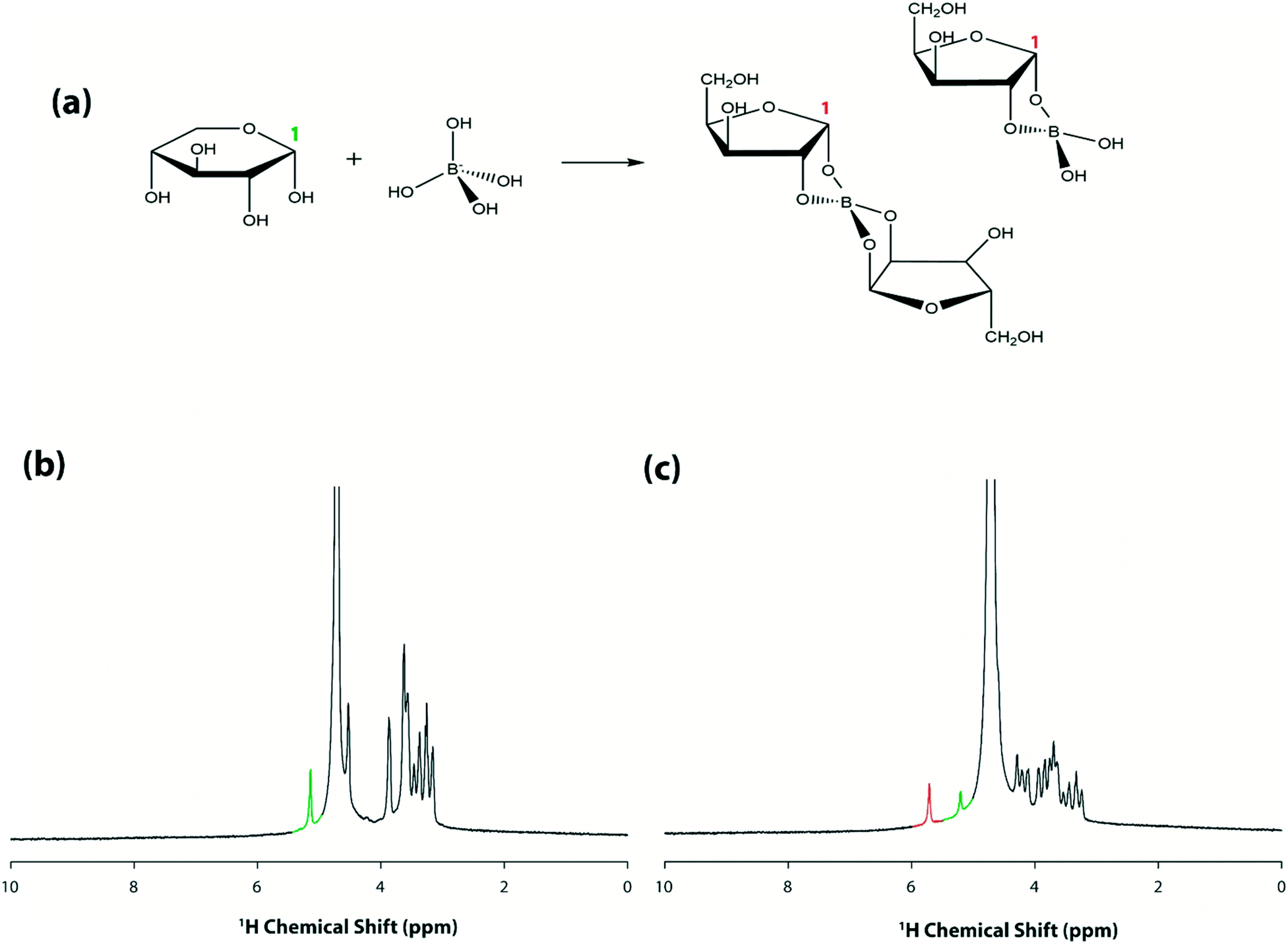
After demonstrating proof-of-concept for remote, in-spectrometer droplet movement, the next goal was to test whether the system could be programmed to initiate and observe a reaction within the spectrometer. A borate–xylose reaction was chosen for this test, in which aqueous borate complexes with the sugar as illustrated in Fig. 5(a). This system is particularly interesting, as it represents a class of reactions that is being explored for applications in saccharide sensors and carbohydrate separations.⁴⁰ As described in the experimental section, separate droplets containing xylose and borate were loaded onto a device and then inserted into the spectrometer. Working remotely, the droplet containing xylose was made to move over the microcoil surface to obtain a spectrum before the reaction was initiated (Fig. 5(b)). As shown, spectra generated under this condition have only one peak (highlighted in green) downfield of the solvent peak, corresponding to the proton at position 1 (5.2 ppm). The two reagents were then mixed by merging the droplet and repeatedly cycling the merged droplet around the device³⁹ for 30 s. A representative spectrum generated from the mixed droplet is shown in Fig. 5(c). As shown, the peak intensity of the non-complexed proton (highlighted in green) is reduced, and a new peak at around 5.7 ppm corresponding to the borate–xylose complex is observed (highlighted in red). This downfield shift in resonance for the proton at carbon 1 is consistent with previous studies,⁴⁰ reflecting the change in the chemical environment upon complexation. The process represented by the data in Fig. 5 was repeated several times (on different devices), and represents the first example (to our knowledge) of a micro-volume reaction initiated within a spectrometer in a batch reactor-fashion (i.e., with no flow).

Fig. 5 DMF–NMR for in-spectrometer reactions. (a) Reaction scheme for borate–xylose complexation, which induces a downfield shift for the proton at carbon 1. Representative DMF–NMR spectra for (b) a droplet of 15 mg mL⁻¹ xylose solution prior to reaction and (c) a merged droplet containing 7.5 mg mL⁻¹ xylose and 1.5 mg mL⁻¹ borate after mixing inside the spectrometer. The peaks highlighted in green and red are assigned to the proton at xylose carbon-1 before and after complexation, respectively.

Finally, the capacity for the new system to follow a reaction time-course was probed using a glucose oxidase reaction, a system that is important in health and diagnostics, and one that has also been studied in microchannel-NMR devices.⁴¹ The scheme for this reaction is shown in Fig. 6(a); note that horseradish peroxidase was also included in the mixture to catalyze the breakdown of H₂O₂ into O₂ (removing products and supplying more reagents to improve the kinetics of the reaction). A reaction time course generated using the new method is shown in Fig. 6(b). The downfield shift for the proton at carbon 1 (from ∼3.25 ppm to ∼4.25 ppm) indicates the expected production of D-glucono-1,5-lactone. Note that because this reaction was carried out in batch mode (with reaction time de-coupled from flow rate), the reagent volume required to collect these data (∼4 μL per reaction) was minimal.

Fig. 6 DMF–NMR for time-resolved reaction monitoring. (a) Reaction scheme for the oxidation of glucose mediated by glucose oxidase, which induces a downfield shift for the proton at carbon 1. (b) Representative NMR spectra collected during a DMF–NMR time-course for glucose oxidation, highlighting the downfield shift at carbon 1 as the reaction progresses.

Conclusion

We introduced a method for interfacing digital microfluidics with an NMR microcoil, and described how the system can be used to manipulate droplets within a high-field NMR spectrometer. As proof-of-concept, reactions in microliter volumes were initiated inside the spectrometer, and the time-courses of reactions were followed in a static droplet, de-coupled from flow rate, with no dead volumes. In future work we plan to adapt the microcoil design to allow for larger arrays of DMF driving electrodes, a counter-electrode for two-plate DMF operation, as well as exploring other improvements such as the possibility of working in an oil medium to reduce or eliminate magnetic susceptibility mismatches between the droplet and the surrounding medium. Overall, we propose that the study described here opens the door for a wide range of interesting applications that could be combined with DMF going forward including integrated procedures with on-chip pre-concentration, reaction, cleanup, and product recovery.

Acknowledgements

We thank the National Sciences and Engineering Research Council (NSERC) for funding, and Prof. Marcel Utz (Southampton Univ.) for enlightening discussions. We thank Bruker for the generous donation of the custom microcoils. A. R. W. thanks the Canada Research Chair (CRC) program for a CRC.

References

1. A. J. Simpson, D. J. McNally and M. J. Simpson, Prog. Nucl. Magn. Reson. Spectrosc., 2011, 58, 97.
2. A. K. Mittermaier and L. E. Kay, Trends Biochem. Sci., 2009, 34, 601.
3. Y. Cohen, L. Avram and L. Frish, Angew. Chem., Int. Ed., 2005, 44, 520.
4. M. H. Levitt, Spin Dynamics, John Wiley & Sons Ltd, Chichester, 2nd edn. 2012.
5. J. H. Ardenkjaer-Larsen, B. Fridlund, A. Gram, G. Hansson, L. Hansson, M. H. Lerche, R. Servin, M. Thaning and K. Golman, Proc. Natl. Acad. Sci. U. S. A., 2003, 100, 10158.
6. M. E. Merritt, C. Harrison, C. Storey, F. M. Jeffrey, A. D. Sherry and C. R. Malloy, Proc. Natl. Acad. Sci. U. S. A., 2007, 104, 19773.
7. T. L. Peck, R. L. Magin and P. C. Lauterbur, J. Magn. Reson., Ser. B, 1995, 108, 114.
8. V. Badilita, R. C. Meier, N. Spengler, U. Wallrabe, M. Utz and J. G. Korvink, Soft Matter, 2012, 8, 10583.
9. C. Massin, F. Vincent, A. Homsy, K. Ehrmann, G. Boero, P.-A. Besse, A. Daridon, E. Verpoorte, N. F. de Rooij and R. S. Popovic, J. Magn. Reson., 2003, 164, 242.
10. R. Kautz, P. Wang and R. W. Giese, Chem. Res. Toxicol., 2013, 26, 1424.
11. R. A. Kautz, W. K. Goetzinger and B. L. Karger, J. Comb. Chem., 2005, 7, 14.
12. M. Kakuta, D. A. Jayawickrama, A. M. Wolters, A. Manz and J. V. Sweedler, Anal. Chem., 2003, 75, 956.
13. M. V. Gomez, A. M. Rodriguez, A. de la Hoz, F. Jimenez-Marquez, R. M. Fratila, P. A. Barneveld and A. H. Velders, Anal. Chem., 2015, 87, 10547.
14. R. M. Fratila, M. V. Gomez, S. Sýkora and A. H. Velders, Nat. Commun., 2014, 5, 3025.
15. H. Wensink, F. Benito-Lopez, D. C. Hermes, W. Verboom, H. J. G. E. Gardeniers, D. N. Reinhoudt and A. van den Berg, Lab Chip, 2005, 5, 280.
16. K. Ehrmann, N. Saillen, F. Vincent, M. Stettler, M. Jordan, F. M. Wurm, P.-A. Besse and R. Popovic, Lab Chip, 2007, 7, 373.
17. H. Lee, E. Sun, D. Ham and R. Weissleder, Nat. Med., 2008, 14, 869.
18. H. Ryan, S. H. Song, A. Zaß, J. Korvink and M. Utz, Anal. Chem., 2012, 84, 3696.
19. J. Bart, A. J. Kolkman, A. J. O.-D. Vries, K. Koch, P. J. Nieuwland, H. J. W. G. Janssen, J. P. J. M. van Bentum, K. A. M. Ampt, F. P. J. T. Rutjes, S. S. Wijmenga, H. J. G. E. Gardeniers and A. P. M. Kentgens, J. Am. Chem. Soc., 2009, 131, 5014.
20. Y. Maguire, I. L. Chuang, S. Zhang and N. Gershenfeld, Proc. Natl. Acad. Sci. U. S. A., 2007, 104, 9198.
21. J. A. Tang, L. A. O'Dell, P. M. Aguiar, D. Sakellariou and R. W. Schurko, Chem. Phys. Lett., 2008, 466, 227.
22. H. Janssen, A. Brinkmann, E. R. H. van Eck, P. J. M. van Bentum and A. P. M. Kentgens, J. Am. Chem. Soc., 2006, 128, 8722.
23. K. Choi, A. H. C. Ng, R. Fobel and A. R. Wheeler, Annu. Rev. Anal. Chem., 2012, 5, 413.
24. N. M. Lafrenière, J. M. Mudrik, A. H. C. Ng, B. Seale, N. Spooner and A. R. Wheeler, Anal. Chem., 2015, 87, 3902.
25. M. D. M. Dryden, D. D. G. Rackus, M. H. Shamsi and A. R. Wheeler, Anal. Chem., 2013, 85, 8809.
26. A. H. C. Ng, M. Lee, K. Choi, A. T. Fischer, J. M. Robinson and A. R. Wheeler, Clin. Chem., 2015, 61, 420.
27. K.-M. Lei, P.-I. Mak, M.-K. Law and R. P. Martins, Analyst, 2015, 140, 5129.
28. K.-M. Lei, P.-I. Mak, M.-K. Law and R. P. Martins, Analyst, 2014, 139, 6204.
29. D. I. Hoult and R. E. Richards, J. Magn. Reson., 1976, 24, 71.
30. H. Ryan, A. Smith and M. Utz, Lab Chip, 2014, 14, 1678.
31. J. Berthier, Microdrops and Digital Microfluidics, Willian Andrew Inc., Norwich, NY, 2nd edn, 2008.
32. M. Abdelgawad and A. R. Wheeler, Adv. Mater., 2007, 19, 133.
33. M. Abdelgawad, M. W. L. Watson, E. W. K. Young, J. M. Mudrik, M. D. Ungrin and A. R. Wheeler, Lab Chip, 2008, 8, 1379.
34. R. Fobel, C. Fobel and A. R. Wheeler, Appl. Phys. Lett., 2013, 102, 193513.
35. S. P. Rucker and A. J. Shaka, Mol. Phys., 1989, 68, 509.
36. A. J. Shaka, C. J. Lee and A. Pines, J. Magn. Reson., 1988, 77, 274.
37. H. Yang, V. N. Luk, M. Abelgawad, I. Barbulovic-Nad and A. R. Wheeler, Anal. Chem., 2009, 81, 1061.
38. S. S. Zalesskiy, E. Danieli, B. Blümich and V. P. Ananikov, Chem. Rev., 2014, 114, 5641.
39. P. Paik, V. K. Pamula, M. G. Pollack and R. B. Fair, Lab Chip, 2003, 3, 28–33.
40. P. E. S. Smith, K. J. Donovan, O. Szekely, M. Baias and L. Frydman, ChemPhysChem, 2013, 14, 3138.
41. A. Yilmaz and M. Utz, Lab Chip, 2016, 16, 2079.

---

Footnotes

† Electronic supplementary information (ESI) available. See DOI: 10.1039/c6lc01073c

‡ These authors contributed equally.

---