DOI:
10.1039/C6LC00150E
(Paper)
Lab Chip, 2016,
16, 1178-1188
Continuum modeling of hydrodynamic particle–particle interactions in microfluidic high-concentration suspensions
Received
2nd February 2016
, Accepted 23rd February 2016
First published on 23rd February 2016
Abstract
A continuum model is established for numerical studies of hydrodynamic particle–particle interactions in microfluidic high-concentration suspensions. A suspension of microparticles placed in a microfluidic channel and influenced by an external force, is described by a continuous particle-concentration field coupled to the continuity and Navier–Stokes equation for the solution. The hydrodynamic interactions are accounted for through the concentration dependence of the suspension viscosity, of the single-particle mobility, and of the momentum transfer from the particles to the suspension. The model is applied on a magnetophoretic and an acoustophoretic system, respectively, and based on the results, we illustrate three main points: (1) for relative particle-to-fluid volume fractions greater than 0.01, the hydrodynamic interaction effects become important through a decreased particle mobility and an increased suspension viscosity. (2) At these high particle concentrations, particle-induced flow rolls occur, which can lead to significant deviations of the advective particle transport relative to that of dilute suspensions. (3) Which interaction mechanism that dominates, depends on the specific flow geometry and the specific external force acting on the particles.
1 Introduction
The ability to sort and manipulate biological particles suspended in bio-fluids is a key element in contemporary lab-on-a-chip technology.1–7 Such suspensions often contain bio-particles in concentrations so high that the particle–particle interactions change the flow behavior significantly compared to that of dilute suspensions. The main goal of this paper is to present a continuum model of hydrodynamic interaction effects in particle transport of high-concentration suspensions moving through microchannels in the presence of external forces.
One important example of high-concentration suspensions is full blood in blood vessels with diameters in the cm to sub-millimeter range or in artificial microfluidic channels. State-of-the-art calculations of the detailed hydrodynamics of blood involve direct numerical simulations (DNS).8–11 DNS models can simultaneously resolve the deformation dynamics of the elastic cell membranes of up to several thousand red blood cells (RBCs) as well as the inter-cell hydrodynamics of the fluid plasma, all in full 3D.9 However, such calculations require a steep price in computational efforts, as large computer clusters running thousands of CPUs in parallel may be involved,9 and the computations may take days.8 The computational cost may be reduced significantly by continuum modeling. Lei et al.12 investigated the limit of small ratios a/H of the particle radius a and the container size H. They found that, to a good approximation, continuum descriptions are valid for a/H ≲ 0.02. This is used in the computationally less demanding approach called mixture theory, or theory of interacting continua, where blood flow is modeled as two superimposed continua, representing the plasma and RBCs.13,14 In a recent study, Kim et al.14 used the method to simulate blood flow in a microchannel, and the results compared favorably to experiments. However, it is debated how to correctly calculate the coupling between the two phases, as well as formulate the stress tensor for the solid phase RBCs. This is called the ‘closure problem’ of mixture theory.15
Another important example is the hydrodynamics of macroscopic suspensions of hard particles, such as in gravity-driven sedimentation. These systems have been described by effective-medium theories of the effective viscosity of the suspension and of the effective single-particle mobility. The textbook by Happel and Brenner16 summarizes work from 1920 to 1960, in particular unit-cell modeling and infinite-array modeling, both approaches imposing a regular distribution of particles. Later, Batchelor17 improved the effective-medium models by applying statistical mechanics for irregularly places particles. In 1982, Mazur and Van Saarloos18 developed the induced-force method for explicit calculation of the hydrodynamic interactions between many rigid spheres. A few years later, this method was extended by Ladd19,20 to allow for a higher number of particles to be considered in an efficient manner. In 1990, Ladd21 used the induced-force method in high-concentration suspensions to calculate three central hydrodynamic transport coefficients: the effective suspension viscosity η, the particle diffusivity D, and the particle mobility μ. The obtained results compare well with both experiments and with preceding theoretical work.
While studies of high-density suspensions with active transport are very important in lab-on-a-chip systems, such as in electro-, magneto-, and acoustophoresis,1,3,4,22 they have not been treated by the microfluidic DNS-models mentioned above. On the other hand, while the effective-medium theories do treat active transport, they have rarely been used to analyze microfluidic systems. In this work, we present a continuum model of high-density suspensions in microchannels exposed to an external force causing particle migration. Based on the results of Lei et al.12 mentioned above, we are justified to use the computationally less demanding continuum description in not too small microfluidic channels, a/H ≲ 0.02. Moreover, with the hydrodynamic transport coefficients obtained by Ladd,21 we can fairly easy write down the governing equations for high-density suspensions following the Nernst–Planck-like approach presented by Mikkelsen and Bruus,23 but here extended to include the hydrodynamic particle–particle interactions.
We establish a continuum effective-medium theory, in which the hydrodynamic interactions between particles in a high-density suspension flowing through a microchannel are modeled by including the concentration dependency of the effective suspension viscosity, the particle diffusivity and mobility, and the transfer of momentum from the particles to the suspension. We then illustrate the use of the theory by two examples: The first is strongly inspired by the magnetophoretic device studied by Mikkelsen and Bruus.23 The second is taken from the emerging field of acoustofluidics24,25 and involves an acoustophoretic device, for which the dilute limit is well described,26–28 but where the behavior in the high-concentration limit is still poorly characterized.
2 Theory
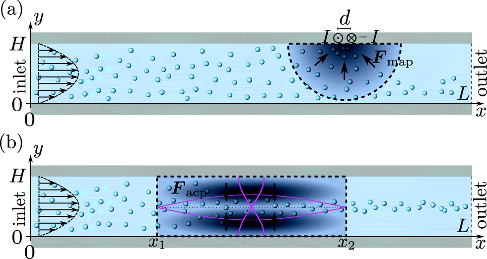
We consider a microchannel at ambient temperature, such as the one sketched in Fig. 1. In a steady-state pressure-driven flow of average inlet velocity v0, an aqueous suspension of microparticles, with the homogeneous concentration c0 (number of particles per volume) at the inlet, is flowing through the microchannel. Only a section of length L is shown. The effects of side-walls, present in actual systems, are negligible for channels with a large width-to-height ratio. Localized in the channel is an active area, where the microparticles are subjected to a transverse single-particle migration force Fmig. This force changes the particle distribution, resulting in an inhomogeneous distribution downstream towards the outlet. In this process, the particles are transported by advection, active migration, and diffusion, all of which are affected by hydrodynamic particle–particle interactions at high concentrations.
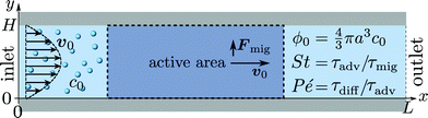 |
| | Fig. 1 Sketch of the model system. Spherical microparticles of diameter 2a are suspended in a Newtonian fluid with a homogeneous number concentration c0, or volume fraction  . The suspension enters from the inlet with velocity v0 and flows towards the localized active area, where the particles experience a transverse migration force Fmig, which redistributes the particles before they leave the channel at the outlet. The resulting particle transport is determined by the relative strength between particle diffusion, advection and migration, which is characterized by three dimensionless numbers: the particle concentration ϕ0, the transient Strouhal number St, and the Péclet number Pé. . The suspension enters from the inlet with velocity v0 and flows towards the localized active area, where the particles experience a transverse migration force Fmig, which redistributes the particles before they leave the channel at the outlet. The resulting particle transport is determined by the relative strength between particle diffusion, advection and migration, which is characterized by three dimensionless numbers: the particle concentration ϕ0, the transient Strouhal number St, and the Péclet number Pé. | |
2.1 Model system
As a simple generic model system, we consider a section of length L of a microchannel with constant rectangular cross-section of height H and width W. In specific calculations we take L = 7H and study for simplicity the flat-channel limit W = 10H, for which the system, in a large part of the center, is reasonably well approximated by a parallel-plate channel. We take the microparticles to be rigid spheres with diameter 2a. Their local concentration (number per volume) is described by the continuous field c(r), but often it is practical to work with the dimensionless concentration (particle volume fraction),| |  | (1) |
We are particularly interested in high inlet concentrations ϕ0 between 0.001 and 0.1, and for this range with the typical values 2a = 2 μm and H = 50 μm, the number of particles in the volume L × W × H is between 104 and 106, which in practice renders direct numerical simulation of the suspension infeasible. We therefore employ continuum modeling in terms of the three continuous fields: the particle concentration c(r), the pressure p(r), and the velocity ν(r) of the suspension.
2.2 Forces and effective particle transport
Our continuum model for the particle current density J includes diffusion (diff), advection (adv), and migration (mig),29 for which we include hydrodynamic particle–particle interactions through c(r),| | | J = Jdiff + Jadv + Jmig | (2a) |
| | | = −D(c)∇c + cν + cμ(c)Fmig | (2b) |
| | | = −χD(ϕ)D0∇c + cν + cχμ(ϕ)μ0Fmig. | (2c) |
Here,| | | D(c) = χD(ϕ)D0 and μ(c) = χμ(ϕ)μ0 | (2d) |
is the effective single-particle diffusivity and mobility, respectively, χD(ϕ) and χμ(ϕ) are concentration-dependent correction factors described in more detail in section 2.5, while μ0 = (6πη0a)−1 and D0 = kBTμ0 is the dilute-limit mobility and diffusivity, respectively, where kB is the Boltzmann constant, T is the temperature, and η0 is the dilute-limit viscosity of the suspension. We do not in this work consider any effects of van der Waals interactions or steric interactions.29 Due to conservation of particles, the particle current density obeys a steady-state continuity equation,
2.3 Effective viscosity and flow of the suspension
The flow of the suspension is governed by the continuity equations for momentum and mass. Treating the suspension as an effective continuum medium with the particle concentration ϕ(r), its density and viscosity are| | | ρ(ϕ) = χρ(ϕ) ρ0 and η(ϕ) = χη(ϕ)−1η0, | (4) |
with the dimensionless correction factors χρ(ϕ) and χη(ϕ)−1 in front of the density ρ0 and viscosity η0 of pure water, respectively. A given particle experiences a drag force, when it is moved relative to the suspension by the migration force Fmig, and in turn, an equal but opposite reaction force is exerted on the suspension. In the continuum limit this is described by the force density cFmig. In steady state, the momentum continuity equation for an incompressible suspension with the stress tensor σ therefore becomes| | | 0 = ∇·[σ(ϕ) − ρ(ϕ)νν] + cFmig, | (5a) |
| | | σ(ϕ) = −1p + χη(ϕ)−1η0[∇ν + (∇ν)T], | (5b) |
where 1 is the unit tensor. Likewise, the steady-state mass continuity equation for an incompressible suspension is written as
2.4 Boundary conditions
We assume a concentration c = c0 and a parabolic flow profile  at the inlet, and vanishing axial gradients ∂xc = 0 and ∂xν = 0 at the outlet. At the walls, we assume a no-slip condition ν = 0, while the condition for c depends on the specific physical system. Lastly, we fix the pressure level to be zero at the lower corner of the outlet p(L, 0) = 0.
2.5 Dimensionless, effective transport coefficients
The dependency of the effective diffusion, mobility, viscosity and density on the particle concentration ϕ is described by the correction factors χD(ϕ), χμ(ϕ), χη(ϕ), and χρ(ϕ), respectively, which can be interpreted as dimensionless effective transport coefficients. The suspension density is a weighted average of the water density ρ0 and the particle density ρp,  . For bio-fluids, particles are often neutrally buoyant, so ρp ≈ ρ0 and χρ ≈ 1. In a comprehensive numerical study of finite-sized, hard spheres suspended in an Newtonian fluid at low Reynolds numbers (the Stokes limit), the remaining transport coefficients χD, χμ, and χη were calculated by Ladd21 at 14 specific values of ϕ between 0.001 and 0.45. For each of the coefficients χ, we have fitted a fourth-order polynomial to the discrete set of values χ−1, while imposing the condition χ(0)−1 = 1 to ensure agreement with the dilute-limit value,
| | χη(ϕ)−1 = 1 + 2.476(7)ϕ + 7.53(2)ϕ2 − 16.34(5)ϕ3 + 83.7(3)ϕ4 + ![[scr O, script letter O]](https://www.rsc.org/images/entities/i_char_e52e.gif) (ϕ5), (ϕ5), | (7a) |
| | | χD(ϕ)−1 = 1 + 1.714(3)ϕ + 6.906(13)ϕ2 − 17.05(3)ϕ3 + 61.2(1)ϕ4 + (ϕ5), | (7b) |
| | | χμ(ϕ)−1 = 1 + 5.55(3)ϕ + 43.4(3)ϕ2 − 149.6(9)ϕ3 + 562(3)ϕ4 + (ϕ5), | (7c) |
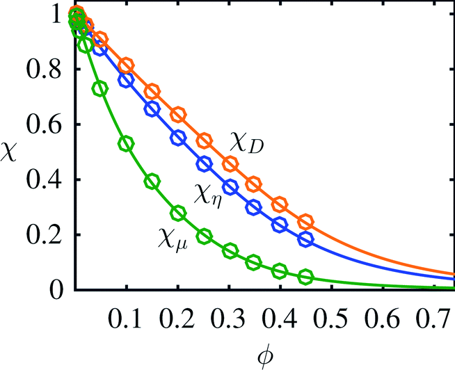
where the uncertainty of the last digit is given in the parentheses. To quantify the quality of the fits χfit compared to the simulated data points χdata, we calculated the relative difference  . We found the standard deviation of Δχ to be 0.003, 0.0019 and 0.0058 for χη, χD and χμ, respectively. Thus, the fourth-order polynomials describe the data points well. The resulting fits from eqn (7) and the original data points21 are plotted in Fig. 2. Note that the mobility χμ is the most rapidly decreasing function of concentration ϕ.
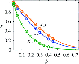 |
| | Fig. 2 Plot of the fitted dimensionless effective transport coefficients χη, χD and χμ as a function of concentration ϕ. The full lines represent the fits from eqn (7), while the circles are the original 14 simulation data points by Ladd.21 | |
We note that the dilute-limit relation  and the definitions μ = χμμ0 and η−1 = χηη0−1 do not imply equality of χμ and χη. In fact, χμ < χη, which highlights the complex nature of the interaction problem at high densities.
2.6 Dimensionless parameters
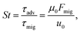
The dynamics of the system can be characterized by three dimensionless numbers. One is the particle concentration ϕ0, which is a measure of the magnitude of the hydrodynamic interactions. The other two are related to the relative magnitude of the diffusion, advection and migration current densities in eqn (2), each characterized by the respective time scales 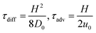 , and
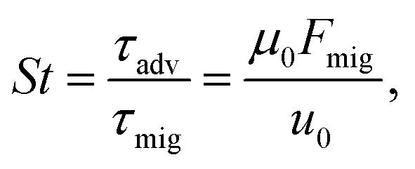
, and  . A small time scale means that the corresponding process is fast and thus dominating. The importance of advection relative to diffusion and of migration relative to advection is characterized by the Péclet number and the transient Strouhal number, respectively,
| | 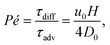 | (8a) |
| |  | (8b) |
| |  | (8c) |
3 Numerical implementation
Following Nielsen and Bruus,30 we implement the governing eqn (2)–(6) in the general weak-form PDE module of the finite element software COMSOL Multiphysics v. 5.0.31 To avoid spurious, numerically induced, negative values of c(r) near vanishing particle concentration, we replace c by the logarithmic variable s = log(c/c0). This variable can assume all real numbers, and it ensures that c = c0![[thin space (1/6-em)]](https://www.rsc.org/images/entities/char_2009.gif) exp(s) is always positive. We implement the weak form using Lagrangian test functions of first order for p and second order for s, vx, and vy.
exp(s) is always positive. We implement the weak form using Lagrangian test functions of first order for p and second order for s, vx, and vy.
A particular numerical problem needs to be taken care of in dealing with the advection in our system. The typical average flow speed is u0 = 200 μm s−1 in our channels of height H = 50 μm, corresponding to a Péclet number Pé = 1.7 × 10⁴. To resolve this flow numerically, a prohibitively fine spatial mesh is needed. However, this problem can be circumvented by artificially increasing the particle diffusivity to χD = 50 instead of using eqn (7b). This decreases the Péclet number to Pé = 2.3 × 10², but since Pé ≫ 1 for both the actual and the artificial diffusivity, advection still dominates in both cases, and as discussed in appendix A, the simulation results for the artificial diffusivity are accurate, but a coarser mesh suffices. In this highly advective regime Pé ≫ 1, the detailed transport in the active area depends on the remaining parameters: the transient Strouhal number St and the inlet concentration ϕ0.
More details on the numerical implementation are given in appendix A.
4 Model results and discussion
To exemplify our continuum effective-medium model, we present two examples using the same channel geometry, but different particle migration mechanisms, namely magnetophoresis (MAP) and acoustophoresis (ACP). The magnetophoresis model is the one introduced by Mikkelsen and Bruus,23 but here extended to include the concentration dependence of the effective transport coefficients χ introduced in section 2.5. This model primarily serves as a model validation. The acoustophoresis model is inspired by the many experimental works reported in Lab on a Chip.24,32–35
4.1 Results for magnetophoresis (MAP)
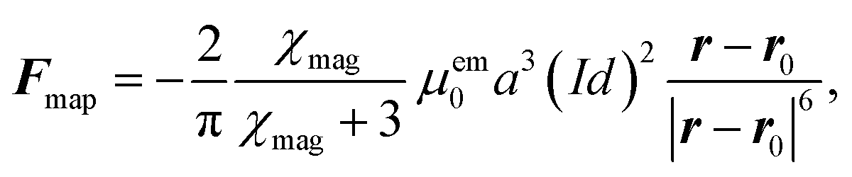
As in Mikkelsen and Bruus,23 we consider the parallel-plate system sketched in Fig. 3(a) of height H = 50 μm, length L = 350 μm, and the boundary conditions of section 2.4. The particles are paramagnetic with magnetic susceptibility χmag = 1 and diameter 2a = 2 μm. A pair of long parallel thin wires is placed perpendicular to the xy-plane with their midpoint at r0 = (x0, y0) = (250, 55) μm, separated by d = dex, and carrying electric currents ±I. The currents lead to a magnetic field, which induces a paramagnetic force Fmap on each particle resulting in magnetophoresis. For a particle at position r, the force is given by23| | 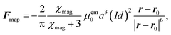 | (9) |
where μem0 is the vacuum permeability. Note how the rapid fifth-power decrease as a function of the wire distance |r − r0|, signals that Fmap is a short-ranged local force. Dipole–dipole interactions are neglected. Using the expression for Fmap, we can determine the migration time τmig for a particle to migrate vertically from the channel center  , directly below the wires, to the wall (x, y) = (x0, H). From this we infer the magnetic transient Strouhal number Stmap,
| |  | (10) |
 |
| | Fig. 3 Specific realizations of the generic system shown in Fig. 1 with height H = 50 μm and length L = 350 μm. The microparticles are rigid spheres of diameter 2a = 2 μm and a paramagnetic susceptibility χmag = 1. A Poiseuille flow with mean velocity u0 is imposed at the inlet. (a) Magnetophoresis: a pair of thin long wires carrying electrical currents ±I is placed at the top of the channel 100 μm upstream from the outlet. The resulting magnetic force Fmap (gray scale) attracts the particles towards the wires. (b) Acoustophoresis: a standing pressure half-wave (magenta) is imposed between x1 and x2. The resulting acoustic force Facp (gray scale) causes the particles to migrate towards the pressure node at  . . | |
Wall boundary conditions for the particles.
Following the simplifying model of Mikkelsen and Bruus,23 we assume that once a particle reaches the wall near the wires, it sticks and is thus removed from the suspension. For the upper wall at y = H, we therefore set the total particle flux in the y-direction equal to the active migration Jy = cμFmap,y, while at the passive bottom wall at y = 0, we choose the standard no-flux condition Jy = 0. For short times, this is a good model, but eventually in a real system, the build-up of particles at the wall is likely to occur, which leads to a dynamically change of the channel geometry.
Particle capture as a function of ϕ0 and Stmap.
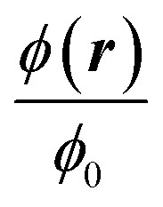
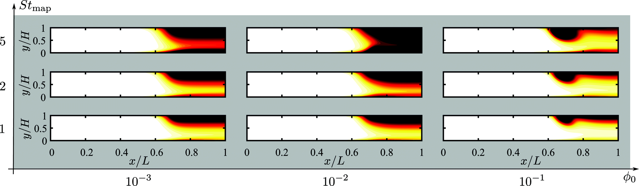
In Fig. 4 we have plotted the normalized steady-state particle concentration  of the system shown in Fig. 3(a) for the nine combinations of ϕ0 = 0.001, 0.01, 0.1 with Stmap = 1, 2, 5. Firstly, it is evident from the figure that for a given fixed ϕ0 and increasing Stmap, an increasing number of particles are captured by the wire-pair, thus decreasing ϕ(r) in a region of increasing size down-stream from the wires. Note also how the slow-moving particles near the bottom wall are pulled upwards by the action of the wires, leaving a decreased particle density there. Secondly, for a fixed Stmap, the particle capture is non-monotonic as a function of ϕ0: it increases going from ϕ0 = 0 via 0.001 to 0.01, but then decreases going from 0.01 to 0.1. Thirdly, for the highest concentration ϕ0 = 0.1, the morphology of the depleted region has changed markedly: a small region depleted of particles forms around the wires at the top wall together with narrow downstream depletion regions along both the top and bottom wall. All three regions increase somewhat in size for increasing Stmap.
 |
| | Fig. 4 Heat color plot of the normalized concentration field  from 1 (white, inlet concentration) to 0 (black, no particles) in the magnetophoretic system Fig. 3(a), for the nine combinations of ϕ0 = 0.001, 0.01, 0.1 with Stmap = 1, 2, 5. from 1 (white, inlet concentration) to 0 (black, no particles) in the magnetophoretic system Fig. 3(a), for the nine combinations of ϕ0 = 0.001, 0.01, 0.1 with Stmap = 1, 2, 5. | |
The normalized capture rate βmap.
We analyze the particle capture quantitatively in terms of the normalized capture rate βmap defined as the ratio between the flux Γtopwall of particles captured on the top wall by the wires, and the flux Γinlet of particles entering through the inlet,23| |  | (11a) |
| |  | (11b) |
where n is the surface normal of a given surface. In Fig. 5(a), we have plotted βmap as a function of ϕ0 for different Stmap values. All of the curves in this plot show the same qualitative behavior: the capture fraction increases with inlet concentration until a certain point, beyond which it declines.
This general behavior is illustrated by the three specific cases ϕ0 = 0.02, 0.045, and 0.1 denoted by the purple bullets A, B and C on the purple “Stmap = 1”-curve. For these three cases, we have in Fig. 5(b1–d1) plotted the magnetically-induced change Δν = ν − ν0 in the suspension velocity, and in Fig. 5(b2–d2) the magnetic force density f = cFmap overlaid by contour lines of c (white). For A in Fig. 5(b1) and (b2) with ϕ0 = 0.02, more particles are captured compared to the dilute case, because cFmap induces a clockwise flow-roll that advects the upstream particles closer to the wires. For B in Fig. 5(c1) and (c2) with ϕ0 = 0.045, cFmap induces two flow rolls, of which the upstream one rotates counter clockwise and advects particles away from the wires, thus lowering the capture compared to A. For C in Fig. 5(d1) and (d2) with ϕ0 = 0.1, cFmap induces a single strong counter-clockwise flow roll that more efficiently advects the upstream particles away from the wires, and βmap decreases further.
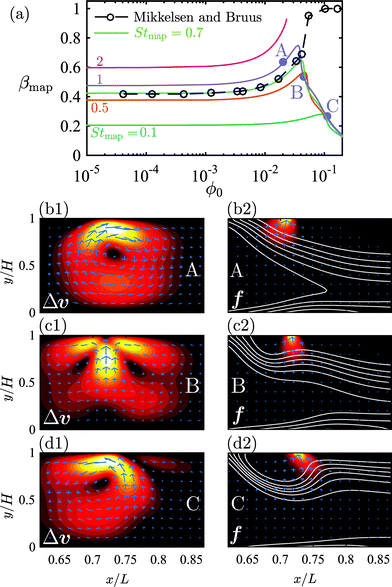 |
| | Fig. 5 (a) Lin–log plot of the capture fraction βmap as a function of the inlet concentration ϕ0 for different transient Strouhal numbers Stmap (full lines). The original results of Mikkelsen and Bruus23 are plotted as circles connected by a dashed line. The purple bullets on the curve for Stmap = 1 mark the three situations A, B, and C plotted in (b)–(d) below. (b1), (c1) and (d1) Color plot from 0 (black) to {1.0, 1.6, 2.0}u0 (white) and vector plot of the particle-induced velocity Δν = ν − ν0 near the wire-pair for situation A, B and C, respectively. (b2), (c2) and (d2) Color plot from 0 (black) to 2 × 10⁵ N m−3 (white) and vector plot of the external force on the suspension f = cFmap. The white lines are contour lines of the concentration field ϕ(r). | |
While the initial increase in βmap for ϕ0 increasing from 0 to 0.03 is in agreement with Mikkelsen and Bruus,23 black circles in Fig. 5(a), the following decrease in βmap for ϕ0 increasing beyond 0.03 was not observed by them. The deviation is not due to our inclusion of the effective transport coefficients χη and χμ, since repeating the simulations23 with χη = χμ = 1 resulted in a curve indistinguishable from the green curve Stmap = 0.7 in Fig. 5(a). We speculate that this deviation is due to our improved mesh resolution.
4.2 Results for acoustophoresis (ACP)
We consider a system identical to the one described in section 4.1, except that the single-particle migration force Fmig now is taken to be the acoustic radiation force Facp arising from the scattering of an imposed standing ultrasound wave on the microparticles. It is given by36| | 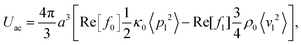 | (12b) |
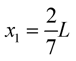
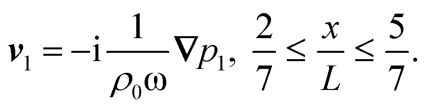
where κ0 and ρ0 is the compressibility and mass density of the carrier fluid, respectively, f0 and f1 are two scattering coefficients, a is the particle radius, and 〈p12〉 and 〈v12〉 is the time-average of the squared acoustic pressure and velocity fields in the suspension, respectively. Inspired by experimentally observed localized fields,26 we take the acoustic field to be a standing half-wave resonance localized in the dashed area for x between  and
and  as indicated by the magenta curves in Fig. 3(b),
| | 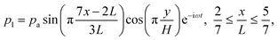 | (13a) |
| | 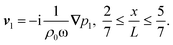 | (13b) |
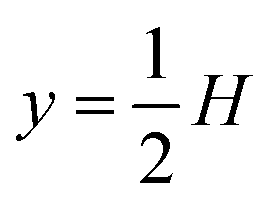
Here, ω = 2πf is the angular actuation frequency with the frequency f typically in the MHz range, and pa is the acoustic pressure amplitude typically in the 0.1 MPa range.26,32 The acoustophoretic force Facp is obtained by inserting the acoustic fields (13) into eqn (12), and the result is a force, which focuses the particles at the pressure node in the channel center at  , see appendix B for details.
Given Facp, we then calculate the transient Strouhal number from the acoustic migration time τmig in the dilute limit (χμ = 1) for a single particle migrating from  to
to  ,26 and from the advection time given by
  ,
,
| | 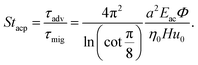 | (14) |
Here,
Eac =
pa2/(4
ρ0cliq2) is the acoustic energy density (typically 1–100 J m
−3),
cliq is the speed of sound in the carrier liquid, and

is the so-called acoustic contrast factor.
37
Wall boundary condition for the particles.
As the particles in this model enter from the inlet, focus towards the channel center  , and leave through the outlet, we choose the simple no-flux boundary condition, n·J|y=0,H = 0, for the bottom and top walls.
Particle capture as a function of ϕ0 and Stacp.
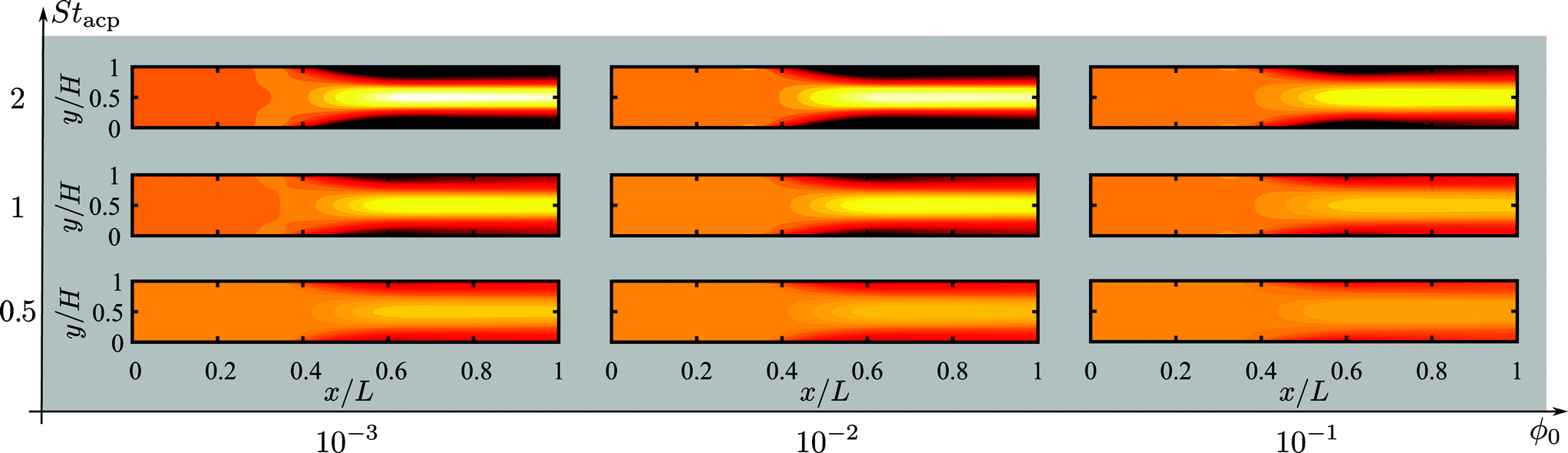
In Fig. 6 is plotted the normalized steady-state particle concentration  of the system shown in Fig. 3(b) for the nine combinations of ϕ0 = 0.001, 0.01, 0.1 to Stacp = 0.5, 1, 2. Clearly, for a given fixed ϕ0 and increasing Stacp, an increasing number of particles are focused in the center region. This is expected since Stacp is proportional to the acoustic energy density Eac. For ϕ0 = 0.001, the center-region concentration (white) is 1.73 times the inlet concentration (orange). Secondly, for a fixed Stacp, the particle focusing is monotonically decreasing as a function of ϕ0 as seen from the decrease in both the width of the particle-free black regions and the magnitude of the downstream center-region concentration. See in particularly the change from ϕ0 = 0.01 to 0.1.
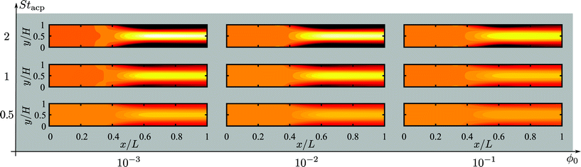 |
| | Fig. 6 Heat color plot of the normalized concentration field  from 1.73 (white, maximum value) to 0 (black, no particles) in the acoustophoretic system Fig. 3(b), for the nine combinations of ϕ0 = 0.001, 0.01, 0.1 with Stacp = 0.5, 1, 2. from 1.73 (white, maximum value) to 0 (black, no particles) in the acoustophoretic system Fig. 3(b), for the nine combinations of ϕ0 = 0.001, 0.01, 0.1 with Stacp = 0.5, 1, 2. | |
To quantify the acoustic focusing for a given inlet concentration, we introduce in analogy with eqn (11) the normalized flux βacp of focused particles leaving through the middle 30% of the outlet,
| |  | (15a) |
| | 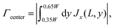 | (15b) |
In the lin–log plot
Fig. 7(a) of
βacpversus ϕ0 for the four Strouhal numbers
Stacp = 0.1, 0.5, 1, and 2, the above-mentioned monotonic decrease in acoustophoretic focusing is clear. Especially for
ϕ0 exceeding 0.01 a dramatic reduction in focusability sets in.
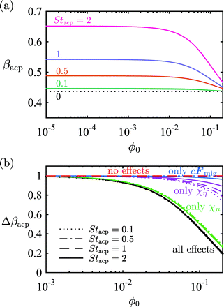 |
| | Fig. 7 (a) Lin–log plot of the acoustic particle focusing fraction βacp (given by eqn (15a)) versus the inlet concentration ϕ0 for four different Stacp values. (b) Lin–log plot of the rescaled particle focusing fraction Δβacp, given by eqn (16), as a function of ϕ0. The line styles denote different Stacp values, and the colors denote the inclusion of one or all hydrodynamic interaction effects, described in section 2. Black: all interaction effects included, green: only effective mobility χμ(ϕ), purple: only effective suspension viscosity χη(ϕ), blue: only momentum transfer from the particles to the suspension cFmig, and red: no interaction effects included. | |
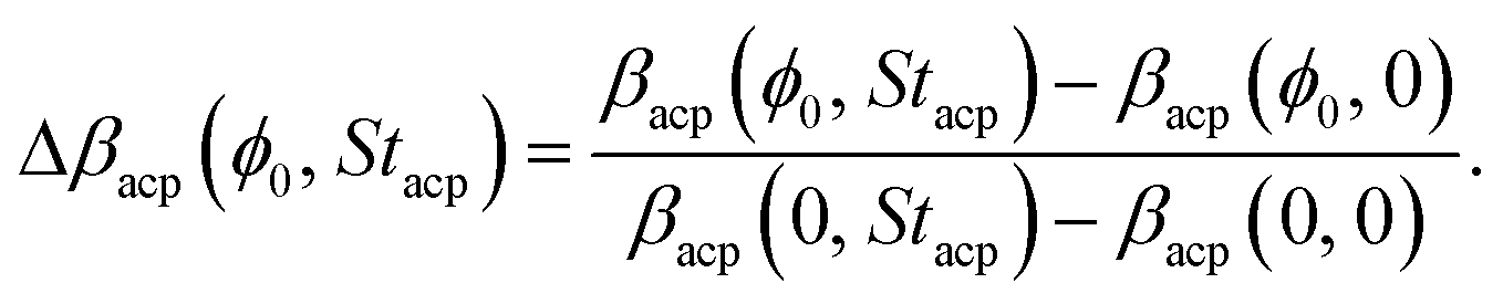
To determine the dominant hydrodynamic interaction mechanism behind this reduction, we introduce the normalized particle focusing fraction Δβacp(ϕ0, Stacp) by the definition,
| |  | (16) |
Here, the difference in normalized center out-flux
βacp at an inlet concentration
ϕ0 between “acoustics on” (
Stacp > 0) and “acoustics off” (
Stacp = 0), is calculated relative to the same difference computed in the dilute limit
cFmig =
0 and
χμ =
χη = 1, which is written as
ϕ0 = 0. We notice that Δ
βacp(
ϕ0,
Stacp) is unity if there is no hydrodynamics interaction effects, and zero if there is no acoustophoretic focusing. In
Fig. 7(b), using the full model (
χμ =
χμ(
ϕ) and
χη =
χη(
ϕ) denoted “all effects”), Δ
βacp is plotted
versus ϕ0 (black lines) for the same four
Stacp values as in
Fig. 7(a). We note that for the full model (black lines), Δ
βacp is almost independent of the strength
Stacp of the acoustophoretic force, which makes it ideal for studying the interaction effects through its
ϕ0 dependency.
To elucidate the origin of the observed reduction in focusability, we also plot the following special cases: “no effects” with χμ = χη = 1 and cFmig = 0 (red lines), “only cFmig” with χμ = χη = 1 (blue lines), “only χη” with χμ = 1 and χη = χη(ϕ) (purple lines), and “only χμ” with χμ = χμ(ϕ) and χη = 1 (green lines). These curves reveal that most of the interaction effect is due to the effective mobility: the green curves “only χμ” are nearly identical to the black curves “all effects”, and both groups of curves show no or little dependence on Stacp. The effective suspension viscosity χη(ϕ) and the particle-induced bulk force cFacp on the suspension only have a minor influence on Δβacp.
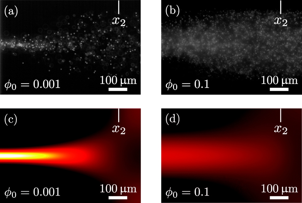
Finally, in Fig. 8 we show the first step towards an experimental validation of our continuum model of hydrodynamic interaction effects. In the figure are seen two micrographs of acoustophoretic focusing of 5.1 μm-diameter polystyrene particles in water in the silicon-glass microchannel setup described in Augustsson et al.26 The micrographs are recorded at Lund University by Kevin Cushing and Thomas Laurell under stop-flow conditions u0 = 0 after 0.43 s of acoustophoresis with the acoustic energy Eac = 102 J m−3. The field of view is near the right edge x2 of the active region sketched in Fig. 3(b). The good focusing obtained at the low density ϕ0 = 0.001 is well reproduced by our model, see Fig. 8(a) and (c). Likewise, the much reduced focusing obtained at the high density ϕ0 = 0.1 is also well reproduced by our model, see Fig. 8(b) and (d). Moreover, which is not shown in the figure, the observed transient behavior of the two cases is also reproduced by simulations: For the low concentration ϕ0 = 0.001, the particles are migrating towards to pressure node directly in straight lines, while for the high concentration ϕ0 = 0.1, pronounced flow rolls are induced, similar to those shown in Fig. 5.
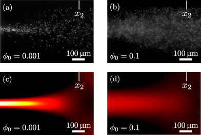 |
| | Fig. 8 Topview near the right edge x2 of the acoustic active region of the particle concentration in a 370 μm-wide microchannel after 0.43 s of acoustophoresis with the acoustic energy Eac = 102 J m−3 on 5.1 μm-diameter polystyrene particles under stop-flow conditions u0 = 0. (a) Experiment with ϕ0 = 0.001. (b) Experiment with ϕ0 = 0.1. (c) Continuum modeling with ϕ0 = 0.001. (d) Continuum modeling with ϕ0 = 0.1. The experimental micrographs courtesy of Kevin Cushing and Thomas Laurell, Lund University. | |
4.3 Discussion
The results of the continuum effective model simulations of the MAP and the ACP models show that the dominating transport mechanisms differ. For the ACP model, the behavior of a suspension in the high-density regime ϕ0 ≳ 0.01 is dominated by the strong decrease in the effective single-particle mobility χμ shown in Fig. 2. Here, the particle–particle interactions are so strong that the suspension moves as a whole with suppressed relative single-particle motion. The response is a steady degradation of the focusing fraction βacp shown in Fig. 7, as it becomes increasingly difficult for a given particle to migrate towards the center line, where the concentration increases and the mobility consequently decreases. In contrast, for the MAP model, the capture fraction βmap increases as ϕ0 increases from 0 to 0.03, confirming the results of Mikkelsen and Bruus.23 The reason for the increased capture is that the particle concentration in the near-wire region is low due to the removal of particles, leaving the single-particle mobility unreduced there, while in the region a little farther away, particles attracted by the wires pull along other particles in a positive feedback due to the high-density “stiffening” of the suspension there. Thus, for the MAP system, the dominating interaction effect is through the particle-induced body force cFmig in eqn (5a).
For ϕ0 increasing beyond 0.03, the observed non-monotonic behavior of βmap and continued monotonic behavior of βacp as a function of increasing ϕ0, depends on whether or not the specific forces and model geometry lead to the formation of flow rolls, such as shown for the MAP model in Fig. 5. The flow-roll-induced decrease observed in the capture efficiency βmap for ϕ0 ≳ 0.03, see Fig. 7(a), was not observed by Mikkelsen and Bruus,23 presumably because of their relatively coarse mesh. For the ACP model, no strong influence from induced flow rolls was observed, and the resulting decrease in focus efficiency was monotonic as a function of ϕ0. This difference in response is caused by differences in spatial symmetry and in the structure of the two migration forces. The MAP model is asymmetric around the horizontal center line, while the ACP model is symmetric, which accentuates the appearance of flow rolls in the former case. Moreover, the rotation of the body force density cFmig can be calculated as ∇ × [cFmig] = c∇ × Fmig − Fmig × ∇c. In the MAP model, both of these rotations are non-zero, while in the ACP model, the first term is zero as Facp is a gradient force, and this feature leads to significant flow rolls in the MAP model and weak ones in the ACP model.
In the above discussion of the results of our model, we have attempted to describe general aspects of hydrodynamic interaction effects, which may be used in future device design considerations. Given the sensitivity on the specific geometry and on the form of external forces, it is clear that detailed design rules are difficult to establish. However, the simplicity of the model allows for relatively easy implementation in numerical simulations of specific device setups.
5 Conclusion
We have presented a continuum effective medium model including hydrodynamic particle–particle interactions, which requires only modest computational resources and time. The results presented in this paper could be obtained in the order of minutes on an ordinary PC. We have validated the model by comparison to previously published models and found quantitative agreement. Moreover, as a first step towards experimental validation, we have found qualitative agreement with experimental observations of acoustophoretic focusing.
Using our numerical model, we have shown that the response of a suspension to a given external migration force depends on the system geometry, the flow, and the specific form of the migration forces. At high densities ϕ0 ≳ 0.01 the suspension “stiffens” and relative single-particle motion is suppressed due to a decreasing effective mobility χμ. However, the detailed response depends on whether or not particle-induced flow rolls appear with sufficient strength to have an impact.
The continuum effective medium model may prove to be a useful and computationally cheap alternative to the vastly more cumbersome direct numerical simulations in the design of lab-on-a-chip systems involving high-density suspensions, for which hydrodynamic particle–particle interactions are expected to play a dominant role.
Appendix A: Numerical implementation, details
The numerical implementation has been carefully checked and validated. To avoid spurious numerical errors, we have performed a mesh convergence analysis as described in details in Muller et al.37 For a continuous field g on a given mesh, we have calculated the relative error 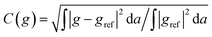 , where gref is the solution obtained for the finest possible mesh. For all fields involved in this study, C falls in the range between 10−5 and 10−3, and it has the desired exponential decrease as function of hmesh−1, where hmesh is the mesh element size. The number of mesh points and degrees of freedom used in our final simulations are listed in Table 1.
Table 1 The number of mesh elements Nmesh, the degrees of freedom DOF, and the mesh Péclet number Pémesh used in the numerical simulations of the MAP and ACP models
| Model |
N
mesh
|
DOFs |
Pémesh |
| MAP |
70000–225000 |
200000–2000000 |
5–10 |
| ACP |
50000–200000 |
400000–2000000 |
5–10 |
We have compared our results with previous work in the literature. Setting χμ = χη = 1, our MAP model in section 4.1 is identical to the one by Mikkelsen and Bruus.23 For this setting, we have calculated the capture fraction βmap as a function of the rescaled quantity (Id)2/u0 (which also appears in the definition (10) for Stmap), and found exact agreement, including the remarkable data collapse, with the results presented in Fig. 3 of Mikkelsen and Bruus.23
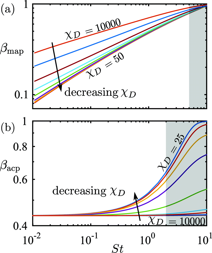
The numerical stability of the finite-element simulation is controlled by the mesh Péclet number Pémesh = hmeshu0/(χDD0) that involves the mesh size hmesh instead of a physical length scale. We found that convergence was ensured for Pémesh ≲ 10, which implies the condition hmesh ≲ 10χDD0/u0 for the mesh size. The higher an advection velocity u0, the finer a mesh is needed. In order to obtain computation times of the order of minutes per variables (Pé, St, ϕ0) on our standard PC, while still keeping Pémesh ≲ 10, we artificially increased χD. In Fig. 9 we have plotted the capture fraction βmap and the focusing fraction βacp as functions of the transient Strouhal number St for χD ranging from 25 to 10000 in the dilute limit with χμ = χη = 1 and cFmig = 0. It is clear from Fig. 9 that the β(St)-curves converge for sufficiently small values of χD. For χD ≤ 50, we determine that acceptable convergence is obtained in both models, and we thus fix χD = 50 for all calculation performed in this work. This choice of χD = 50 allows for acceptable computation times (∼10 min per variable set). In other words, once the Péclet number is sufficiently high, the convergence is ensured by the dominance of advection over diffusion.
 |
| | Fig. 9 Log–log plot of (a) the capture fraction βmap and (b) the focusing fraction βacp, both as a function of the transient Strouhal number St in the dilute limit (χμ = χη = 1 and cFmig = 0) for χD = 25, 50, 100, 200, 500, 100, 2000, 5000, and 10000. Only simulations with St-values outside the gray areas have been included in the analysis of Fig. 4–7. | |
Appendix B: The acoustophoretic force
The acoustophoretic force Facp is found from the gradient of Uac in eqn (12) using the acoustic fields p1 and v1 defined in eqn (13). In Fig. 10 is shown a combined color and vector plot of the resulting force Facp given by the explicit expressions of its components Facp,x and Facp,y,| | 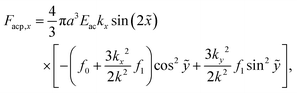 | (17a) |
| | 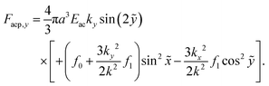 | (17b) |
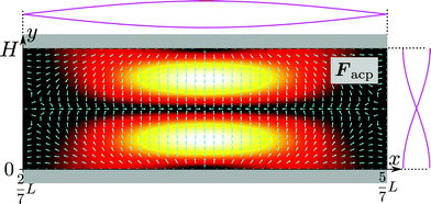 |
| | Fig. 10 The magnitude (heat color plot from zero [black] to maximum [white]) and the direction (vector plot) of the acoustophoretic force Facp given in eqn (17a) and (17b). | |
Here,  and ỹ = kyy are dimensionless coordinates, and kx = 7π/(3L), ky = π/H, and k2 = kx2 + ky2 are wave numbers. For water-suspended polystyrene spheres with radius a ≳ 1 μm, we have f0 = 0.444 and f1 = 0.034.37 The acoustic energy density is set to Eac = 102 J m−3.
Acknowledgements
We thank Kevin Cushing and Thomas Laurell for kindly providing us with the micrographs of Fig. 8(a) and (b). This work was supported by Lund University and the Knut and Alice Wallenberg Foundation (Grant No. KAW 2012.0023).
References
- A. Lenshof, C. Magnusson and T. Laurell, Lab Chip, 2012, 12, 1210–1223, 10.1039/c2lc21256k.
- H. Amini, W. Lee and D. Di Carlo, Lab Chip, 2014, 14, 2739–2761, 10.1039/C4LC00128A.
- T. Z. Jubery, S. K. Srivastava and P. Dutta, Electrophoresis, 2014, 35, 691–713, 10.1039/C4LC01422G.
- M. Hejazian, W. Li and N.-T. Nguyen, Lab Chip, 2015, 15, 959–970, DOI:10.1155/2015/239362.
- W. S. Low and W. A. B. W. Abas, BioMed Res. Int., 2015, 2015, 239362, DOI:10.1155/2015/239362.
- O. Otto, P. Rosendahl, A. Mietke, S. Golfier, C. Herold, D. Klaue, S. Girardo, S. Pagliara, A. Ekpenyong, A. Jacobi, M. Wobus, N. Topfner, U. F. Keyser, J. Mansfeld, E. Fischer-Friedrich and J. Guck, Nat. Methods, 2015, 12, 199–202, DOI:10.1038/nmeth.3281.
- C. W. Shields, C. D. Reyes and G. P. López, Lab Chip, 2015, 15, 1230–1249, 10.1039/c4lc01246a.
- D. A. Reasor, J. R. Clausen and C. K. Aidun, Int. J. Numer. Methods Fluids, 2012, 68, 767–781, DOI:10.1002/fld.2534.
- J. R. Clausen, D. A. Reasor and C. K. Aidun, Comput. Phys. Commun., 2010, 181, 1013–1020, DOI:10.1016/j.cpc.2010.02.005.
- M. Mehrabadi, D. N. Ku and C. K. Aidun, Ann. Biomed. Eng., 2015, 43, 1410–1421, DOI:10.1007/s10439-014-1168-4.
- P. Bagchi, Biophys. J., 2007, 92, 1858–1877, DOI:10.1529/biophysj.106.095042.
- H. Lei, D. A. Fedosov, B. Caswell and G. E. Karniadakis, J. Fluid Mech., 2013, 722, 214–239, DOI:10.1017/jfm.2013.91.
- M. Massoudi, J. Kim and J. F. Antaki, Int. J. Nonlinear Mech., 2012, 47, 506–520, DOI:10.1016/j.ijnonlinmec.2011.09.025.
- J. Kim, J. F. Antaki and M. Massoudi, J. Comput. Appl. Math., 2016, 292, 174–187, DOI:10.1016/j.cam.2015.06.017.
- M. Massoudi, Int. J. Eng. Sci., 2010, 48, 1440–1461, DOI:10.1016/j.ijengsci.2010.08.005.
-
J. Happel and H. Brenner, Low Reynolds number hydrodynamics with special applications to particulate media, Martinus Nijhoff Publishers, The Hague, 1983 Search PubMed.
- G. K. Batchelor, J. Fluid Mech., 1972, 52, 245, DOI:10.1017/S0022112072001399.
- P. Mazur and W. Van Saarloos, Phys. A, 1982, 115, 21–57, DOI:10.1016/0378-4371(82)90127-3.
- A. J. C. Ladd, J. Chem. Phys., 1988, 88, 5051–5063, DOI:10.1063/1.454658.
- A. J. C. Ladd, J. Chem. Phys., 1989, 90, 1149–1157, DOI:10.1063/1.456170.
- A. J. C. Ladd, J. Chem. Phys., 1990, 93, 3484–3494, DOI:10.1063/1.458830.
- B. Cetin, M. B. Ozer and M. E. Solmaz, Biochem. Eng. J., 2014, 92, 63–82, DOI:10.1016/j.bej.2014.07.013.
- C. Mikkelsen and H. Bruus, Lab Chip, 2005, 5, 1293–1297, 10.1039/b507104f.
- H. Bruus, J. Dual, J. Hawkes, M. Hill, T. Laurell, J. Nilsson, S. Radel, S. Sadhal and M. Wiklund, Lab Chip, 2011, 11, 3579–3580, 10.1039/c1lc90058g.
-
T. Laurell and A. Lenshof, Microscale Acoustofluidics, Royal Society of Chemistry, 2014 Search PubMed.
- P. Augustsson, R. Barnkob, S. T. Wereley, H. Bruus and T. Laurell, Lab Chip, 2011, 11, 4152–4164, 10.1039/c1lc20637k.
- R. Barnkob, P. Augustsson, T. Laurell and H. Bruus, Phys. Rev. E: Stat., Nonlinear, Soft Matter Phys., 2012, 86, 056307, DOI:10.1103/PhysRevE.86.056307.
- P. B. Muller, M. Rossi, A. G. Marin, R. Barnkob, P. Augustsson, T. Laurell, C. J. Kähler and H. Bruus, Phys. Rev. E: Stat., Nonlinear, Soft Matter Phys., 2013, 88, 023006, DOI:10.1103/PhysRevE.88.023006.
-
J. K. G. Dhont, An introduction to dynamics of colloids, Elsevier, Amsterdam, 1996 Search PubMed.
- C. P. Nielsen and H. Bruus, Phys. Rev. E: Stat., Nonlinear, Soft Matter Phys., 2014, 90, 043020, DOI:10.1103/PhysRevE.90.043020.
-
COMSOL Multiphysics 5.0, www.comsol.com, 2015 Search PubMed.
- R. Barnkob, P. Augustsson, T. Laurell and H. Bruus, Lab Chip, 2010, 10, 563–570, 10.1039/b920376a.
- M. Wiklund, Lab Chip, 2012, 12, 2018–2028, 10.1039/c2lc40201g.
- M. Nordin and T. Laurell, Lab Chip, 2012, 12, 4610–4616, 10.1039/c2lc40201g.
- M. Antfolk, P. B. Muller, P. Augustsson, H. Bruus and T. Laurell, Lab Chip, 2014, 14, 2791–2799, 10.1039/c4lc00202d.
- M. Settnes and H. Bruus, Phys. Rev. E: Stat., Nonlinear, Soft Matter Phys., 2012, 85, 016327, DOI:10.1103/PhysRevE.85.016327.
- P. B. Muller, R. Barnkob, M. J. H. Jensen and H. Bruus, Lab Chip, 2012, 12, 4617–4627, 10.1039/C2LC40612H.
|
| This journal is © The Royal Society of Chemistry 2016 |
Click here to see how this site uses Cookies. View our privacy policy here. 
 Open Access Article
 This Open Access Article is licensed under a Creative Commons Attribution-Non Commercial 3.0 Unported Licence
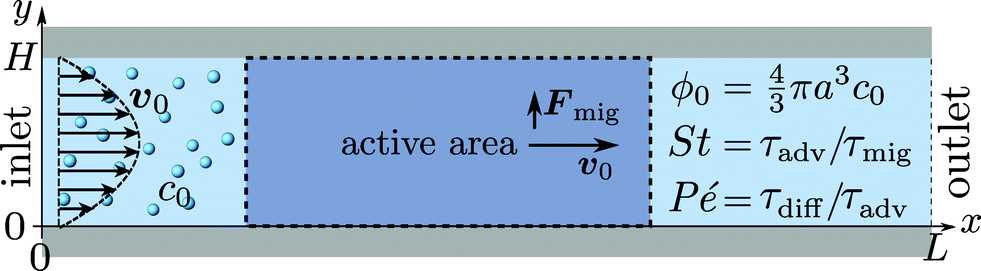
 . The suspension enters from the inlet with velocity v0 and flows towards the localized active area, where the particles experience a transverse migration force Fmig, which redistributes the particles before they leave the channel at the outlet. The resulting particle transport is determined by the relative strength between particle diffusion, advection and migration, which is characterized by three dimensionless numbers: the particle concentration ϕ0, the transient Strouhal number St, and the Péclet number Pé.
 at the inlet, and vanishing axial gradients ∂xc = 0 and ∂xν = 0 at the outlet. At the walls, we assume a no-slip condition ν = 0, while the condition for c depends on the specific physical system. Lastly, we fix the pressure level to be zero at the lower corner of the outlet p(L, 0) = 0.
 . For bio-fluids, particles are often neutrally buoyant, so ρp ≈ ρ0 and χρ ≈ 1. In a comprehensive numerical study of finite-sized, hard spheres suspended in an Newtonian fluid at low Reynolds numbers (the Stokes limit), the remaining transport coefficients χD, χμ, and χη were calculated by Ladd21 at 14 specific values of ϕ between 0.001 and 0.45. For each of the coefficients χ, we have fitted a fourth-order polynomial to the discrete set of values χ−1, while imposing the condition χ(0)−1 = 1 to ensure agreement with the dilute-limit value,
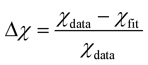 . We found the standard deviation of Δχ to be 0.003, 0.0019 and 0.0058 for χη, χD and χμ, respectively. Thus, the fourth-order polynomials describe the data points well. The resulting fits from eqn (7) and the original data points21 are plotted in Fig. 2. Note that the mobility χμ is the most rapidly decreasing function of concentration ϕ.
 and the definitions μ = χμμ0 and η−1 = χηη0−1 do not imply equality of χμ and χη. In fact, χμ < χη, which highlights the complex nature of the interaction problem at high densities.
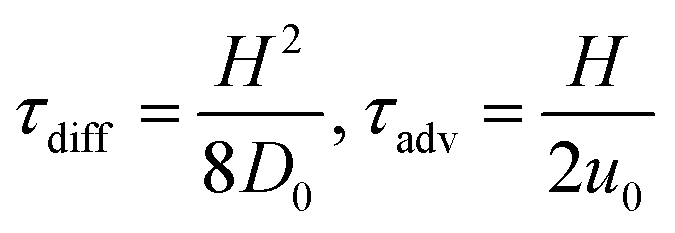 , and
, and 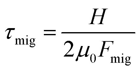 . A small time scale means that the corresponding process is fast and thus dominating. The importance of advection relative to diffusion and of migration relative to advection is characterized by the Péclet number and the transient Strouhal number, respectively,
 , directly below the wires, to the wall (x, y) = (x0, H). From this we infer the magnetic transient Strouhal number Stmap,
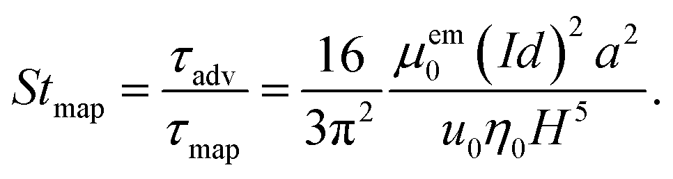
 .
. of the system shown in Fig. 3(a) for the nine combinations of ϕ0 = 0.001, 0.01, 0.1 with Stmap = 1, 2, 5. Firstly, it is evident from the figure that for a given fixed ϕ0 and increasing Stmap, an increasing number of particles are captured by the wire-pair, thus decreasing ϕ(r) in a region of increasing size down-stream from the wires. Note also how the slow-moving particles near the bottom wall are pulled upwards by the action of the wires, leaving a decreased particle density there. Secondly, for a fixed Stmap, the particle capture is non-monotonic as a function of ϕ0: it increases going from ϕ0 = 0 via 0.001 to 0.01, but then decreases going from 0.01 to 0.1. Thirdly, for the highest concentration ϕ0 = 0.1, the morphology of the depleted region has changed markedly: a small region depleted of particles forms around the wires at the top wall together with narrow downstream depletion regions along both the top and bottom wall. All three regions increase somewhat in size for increasing Stmap.
 from 1 (white, inlet concentration) to 0 (black, no particles) in the magnetophoretic system Fig. 3(a), for the nine combinations of ϕ0 = 0.001, 0.01, 0.1 with Stmap = 1, 2, 5.


 and
and  as indicated by the magenta curves in Fig. 3(b),
 , see appendix B for details.
 to
to  ,26 and from the advection time given by
  ,
,
 is the so-called acoustic contrast factor.37
 , and leave through the outlet, we choose the simple no-flux boundary condition, n·J|y=0,H = 0, for the bottom and top walls.
 of the system shown in Fig. 3(b) for the nine combinations of ϕ0 = 0.001, 0.01, 0.1 to Stacp = 0.5, 1, 2. Clearly, for a given fixed ϕ0 and increasing Stacp, an increasing number of particles are focused in the center region. This is expected since Stacp is proportional to the acoustic energy density Eac. For ϕ0 = 0.001, the center-region concentration (white) is 1.73 times the inlet concentration (orange). Secondly, for a fixed Stacp, the particle focusing is monotonically decreasing as a function of ϕ0 as seen from the decrease in both the width of the particle-free black regions and the magnitude of the downstream center-region concentration. See in particularly the change from ϕ0 = 0.01 to 0.1.
 from 1.73 (white, maximum value) to 0 (black, no particles) in the acoustophoretic system Fig. 3(b), for the nine combinations of ϕ0 = 0.001, 0.01, 0.1 with Stacp = 0.5, 1, 2.

 , where gref is the solution obtained for the finest possible mesh. For all fields involved in this study, C falls in the range between 10−5 and 10−3, and it has the desired exponential decrease as function of hmesh−1, where hmesh is the mesh element size. The number of mesh points and degrees of freedom used in our final simulations are listed in Table 1.


 and ỹ = kyy are dimensionless coordinates, and kx = 7π/(3L), ky = π/H, and k2 = kx2 + ky2 are wave numbers. For water-suspended polystyrene spheres with radius a ≳ 1 μm, we have f0 = 0.444 and f1 = 0.034.37 The acoustic energy density is set to Eac = 102 J m−3.