
 Open Access Article
 This Open Access Article is licensed under a
 Creative Commons Attribution 3.0 Unported Licence
Characterization of a series of absolute isotope reference materials for magnesium: ab initio calibration of the mass spectrometers, and determination of isotopic compositions and relative atomic weights†
Jochen
Vogl
*a,
Björn
Brandt
a,
Janine
Noordmann
b,
Olaf
Rienitz
b and
Dmitriy
Malinovskiy
c
aBundesanstalt für Materialforschung und -prüfung (BAM), Richard-Willstätter-Straße 11, 12489 Berlin, Germany. E-mail: jochen.vogl@bam.de
bPhysikalisch-Technische Bundesanstalt (PTB), Bundesallee 100, 38116 Braunschweig, Germany. E-mail: olaf.rienitz@ptb.de
cLGC Limited, Queens Road, Teddington, Middlesex TW11 0LY, UK. E-mail: dmitriy.malinovskiy@lgcgroup.com
First published on 14th April 2016
Abstract
For the first time, an ab initio calibration for absolute Mg isotope ratios was carried out, without making any a priori assumptions. All quantities influencing the calibration such as the purity of the enriched isotopes or liquid and solid densities were carefully analysed and their associated uncertainties were considered. A second unique aspect was the preparation of three sets of calibration solutions, which were applied to calibrate three multicollector ICPMS instruments by quantifying the correction factors for instrumental mass discrimination. Those fully calibrated mass spectrometers were then used to determine the absolute Mg isotope ratios in three candidate European Reference Materials (ERM)-AE143, -AE144 and -AE145, with ERM-AE143 becoming the new primary isotopic reference material for absolute isotope ratio and delta measurements. The isotope amount ratios of ERM-AE143 are n(25Mg)/n(24Mg) = 0.126590(20) mol mol−1 and n(26Mg)/n(24Mg) = 0.139362(43) mol mol−1, with the resulting isotope amount fractions of x(24Mg) = 0.789920(46) mol mol−1, x(25Mg) = 0.099996(14) mol mol−1 and x(26Mg) = 0.110085(28) mol mol−1 and an atomic weight of Ar(Mg) = 24.305017(73); all uncertainties were stated for k = 2. This isotopic composition is identical within uncertainties to those stated on the NIST SRM 980 certificate. The candidate materials ERM-AE144 and -AE145 are isotopically lighter than ERM-AE143 by −1.6‰ and −1.3‰, respectively, concerning their n(26Mg)/n(24Mg) ratio. The relative combined standard uncertainties are ≤0.1‰ for the isotope ratio n(25Mg)/n(24Mg) and ≤0.15‰ for the isotope ratio n(26Mg)/n(24Mg). In addition to characterizing the new isotopic reference materials, it was demonstrated that commonly used fractionation laws are invalid for correcting Mg isotope ratios in multicollector ICPMS as they result in a bias which is not covered by its associated uncertainty. Depending on their type, fractionation laws create a bias up to several per mil, with the exponential law showing the smallest bias between 0.1‰ and 0.7‰.
1. Introduction
Measuring the isotopic composition of an element requires mass spectrometry, and – due to the specifics of mass spectrometers – always requires calibration, e.g. using a suitable reference material, since mass spectrometers in principle do not provide absolute isotope ratios out of themselves. For most cases, it is sufficient that isotopic compositions or isotope ratios be described in terms of the difference between the respective isotope ratio in a standard and the sample relative to the ratio in the standard; those relative values are known as “delta values” – often expressed in per mil (“‰”). For most applications such as authenticity studies,1 or geological surveys,2,3 such relative values are sufficient. Whenever possible, however, the basis of isotope ratio measurements should be absolute isotope ratios, which are invariant in space and time and expressed by the international system of units, SI.Measuring absolute isotopic compositions, however, requires the calibration of mass spectrometers by primary isotopic reference materials, which in turn requires the certification of such a material. Since mass spectrometers suffer from a number of effects that influence their absolute sensitivity, the isotopic composition is usually measured and described in terms of ratios of signals of two isotopes, since those ratios are typically more stable than one signal alone, and thus is more meaningful in day-to-day comparison. In ICP instruments, the instability of the plasma ionization source results in large signal variations; as a result, measuring isotope signals on one detector and switching between isotopes in the measurement sequence can result in a large bias and uncertainties. To overcome these drawbacks, the isotopes are measured simultaneously using two or more Faraday cups (collectors); this allows removal of the influence of plasma intensity fluctuations since all signals are measured at the same time, and are thus influenced by the same variation.
The typical mass spectrometers used for experimental determinations of the isotopic composition are thus multi-collector instruments (TIMS and ICPMS), but as any other mass spectrometer they suffer from a number of bias effects that result in a varying skew of isotopic signal ratios measured over the mass range; until today, it is impossible to describe this skew with sufficient detail that would allow us to model, to accurately predict and thus to correct the value for a specific isotope. Consequently, it is until today impossible to transfer the calibration for one isotope to another isotope, even if it immediately neighbours a calibrated isotope. Thus, the relative instrumental response needs to be calibrated for all simultaneously collected ion beams.4 For elements of multiple stable isotopes, a number of isotope ratios need to be calibrated for. This requires a complex measurement strategy, in which the sample(s) are compared with the standards (calibration solutions); time-dependent instabilities of the instruments can quickly impact the accuracy of the calibration in this case, since adequate sequences can easily last a number of hours. Since isotopically enriched samples are used in this sequence, changes of blank values can influence the overall results significantly, and further complicate the sequences. The full requirements of such an absolute calibration, and the basic measurement concept used in this case (the synthetic isotope calibration approach by Alfred O. C. Nier5) have been described in more detail in a prior publication.4
Alternatively, measuring delta values is much simpler, since it usually only requires comparing intensity ratios with respect to a standard, which is usually a natural sample with no isotopic enrichment (thus not resulting in significant changes of the blank values due to isotopically enriched samples). Since the sample can be completely characterized in just one measurement (using the known bracketing approach6) – instead of measuring a number of standards for each relevant isotope ratio (as in the case of absolute calibration) – such measurements are usually easier conducted, and do not suffer from the same type of signal drift and instrument instability. However, absolute values can only be obtained from delta values if the standard has been characterized with respect to its absolute isotopic composition – which most standards have not been. Consequently, such measurements are not an option themselves to determine absolute isotopic compositions.
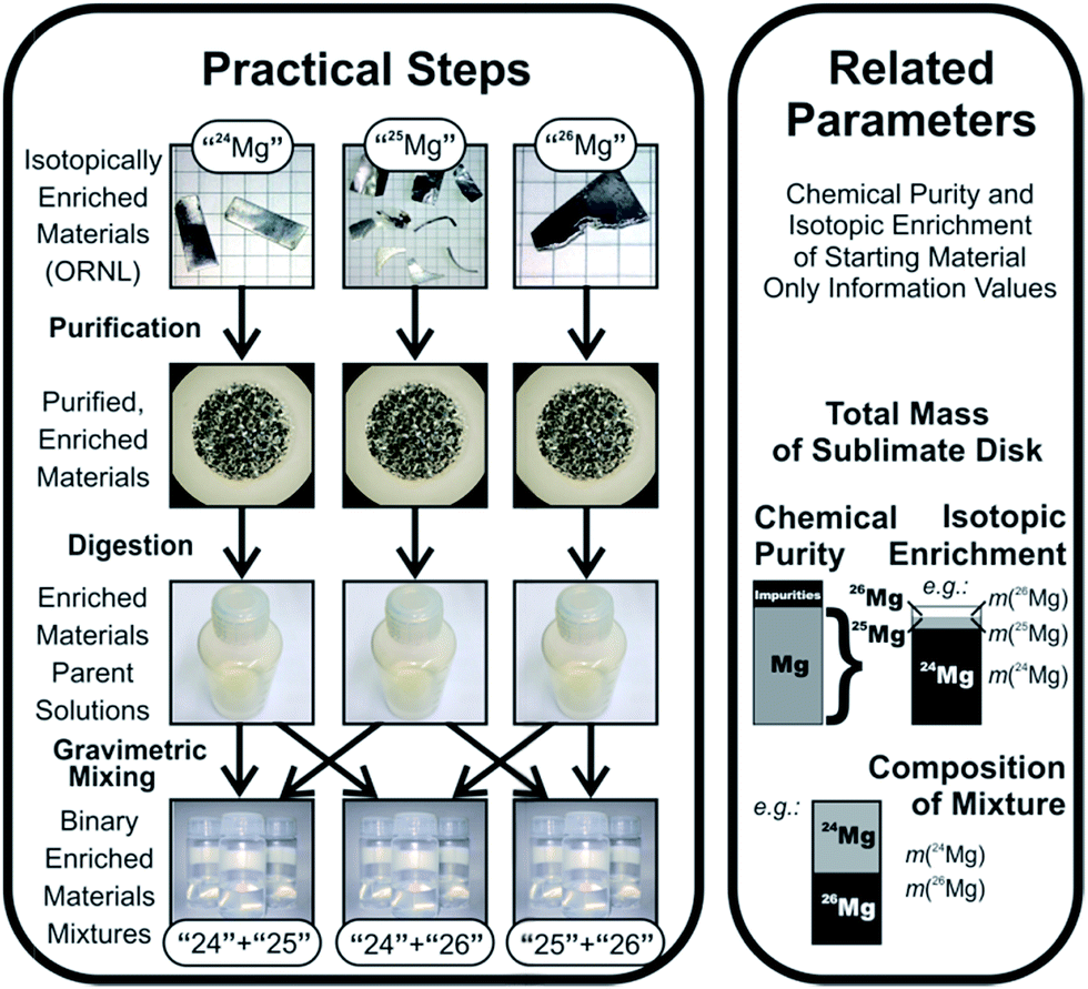
In this work, we want to characterize three candidates for a new absolute isotopic reference material, which can then be used to determine absolute isotope ratios and delta values as well. Since we need to perform an absolute calibration, we need to conduct complex mass spectrometric sequences on a multi-collector ICPMS instrument. Magnesium, which consists of three stable isotopes, 24Mg, 25Mg and 26Mg, has been chosen as a target element due to the following three reasons: (1) the inhomogeneity of the primary Mg isotope reference material NIST SRM 980,7 (2) the lack of suitable isotope reference materials and (3) the increasing number of Mg isotope ratio measurements.4 Suitable calibration solutions with uncertainties low enough to enable the certification of natural standards with uncertainties at least equal to or better than the ones currently available have been prepared in a prior project, which are described in ref. 4. The calibration concept is shown in Fig. 1.
 | ||
| Fig. 1 Calibration concept, reproduced from ref. 4 with permission from the Royal Society of Chemistry. | ||
In this work, we have used those calibration solutions to calibrate three mass spectrometers in three institutes, and to determine the absolute isotopic composition in three candidates. The three partner laboratories were given much freedom to devise their own protocol for the measurement sequences, in light of the above-mentioned issues in their design; also the data pre-processing (blank subtractions, etc.) was conducted in the three labs. Finally, the data evaluation has been conducted in a centralized manner, using an analytical approach, and a complete uncertainty budget – which uses the uncertainties of the calibration solutions as well as the standard uncertainties of the measurements from this project as input values. The final expanded uncertainty of an isotope reference material mainly depends on the homogeneity, stability and characterization measurements. Since we provide mono-elemental solutions, homogeneity and stability issues can be solved easily,8,9 and only the characterization measurements remain a source of uncertainty, which in turn depend on the isotope ratio repeatability of the selected mass spectrometer and the uncertainty of the calibration. The isotope ratio repeatability of the chosen MC-ICPMS Neptune (Plus) is better than 0.01% for Mg isotope ratio measurements, as our previous tests showed. The uncertainty of the calibration only derives from the uncertainty introduced during the preparation of the isotope mixtures used for calibration, for which relative expanded uncertainties of better than 0.007% have been determined in the preceding project.4 Putting the uncertainties of the calibration solutions and the isotope ratio measurements together, the project's target uncertainty of <0.05% (relative, k = 2) for the magnesium isotope reference material was considered to be achievable.
2. Methods, instrumentation, and software
2.1 Uncertainty budgets
Determinations of uncertainties of the primary descriptor values are the central task in this project, since the final values of the project, the isotopic composition of the candidate Isotopic Reference Materials (IRMs) alone, are worthless without an associated uncertainty. All determinations of uncertainties are based strictly on the principles described in the Guide to the Expression of Uncertainty in Measurement (GUM), as published by the members of the Joint Committee for Guides in Metrology.10 In practice, those parameters are calculated based on a propagation of the uncertainties of the input values using linearization of the describing equations, based on commercial application software (GUM Workbench, V 2.4, Metrodata GmbH, Weil am Rhein, Germany11); further details have been described in a previous publication.42.2 Basic laboratory equipment, and practices
The basics about labware and handling protocols are the same as those in the preceding project on the preparation of the calibration solutions, and all steps are described in detail in ref. 4.The basic features of our experimental approach are summarized as follows: the use of analytical grade chemicals; acids are further purified by two-stage sub-boiling distillation. Ultra-pure water is used (Milli-Q). All substances and liquids are stored in low-particulate fluoropolymer (PFA or FEP) containers (Nalgene, Savillex and Sanplatec); a dedicated cleaning protocol is used for those containers. For most solutions in this project, newly purchased containers have been obtained; the only exception being dilute acids, where in some cases, laboratory containers have been used that are only used for this ultra-pure acid.
Except for the finishing (final dilution) of measurement solutions, all procedures are conducted gravimetrically; this includes the digestion and dilution of candidates, and the preparation of acids. Weighing is of utmost significance to the success of the current project, and extreme care has been taken to conduct weighing to obtain correct weighing results. Details about weighing protocols, hardware, calibrations/uncertainties and buoyancy correction are described in the previous publication; the same protocols and instrumentation have been applied in the present work, with the exception of the weighing of the candidates ERM-AE-143 and -AE144 (see below), for which the balance Mettler Toledo UMT-5 was used (also at BAM). This balance is very similar to balance UMT-2 (used in the previous part), and is also calibrated the same way, including a certified calibration protocol based on OIML class E2 weights.
Unlike the prior project part, the quality of the candidate solutions prepared in this second part is not of the same significance for the uncertainties of the end result as the quality of the calibration solutions prepared in the first part. The solutions in this second part, however, have still been prepared with the same care. For digestion and dilution, the acids from the first project (0.06 g g−1 HNO3, 0.02 g g−1 HNO3 in the 5 L batch) were used.
The measurement solutions were then distributed to the partner labs in cleaned PFA containers. The acid used for diluting the stock solutions down to the measurement concentration was newly prepared volumetrically from ultra-pure acids. Aliquots of the acid used for dilution were sent to the partner lab for blank measurements. In the case of BAM (the coordinating lab in this case), the same acid was used for the preparation of the candidate dilutions, and for the dilution of the calibration solutions. This acid, thus, is also used for the blank measurements at BAM. All characteristics of the acids used in this project such as the magnesium blank and density are listed in ref. 4.
2.3 Selection and handling of candidate materials
Three natural magnesium samples were selected as candidates for the to-be-delivered Mg absolute isotopic reference materials, where ERM is a registered trademark and stands for the European Reference Material, “A” denotes a non-matrix material and “E” an isotope material. An overview is given in Table 1.| Parameter | Candidate | Candidate | Candidate |
|---|---|---|---|
| ERM-AE143 | ERM-AE144 | ERM-AE145 | |
| a Nominal purity provided by producer/supplier. b Based on glow discharge mass spectrometry (GDMS) measurements. c Based on GDMS measurements of parallel sublimated samples. | |||
| Source | Alfa Aesar | Alfa Aesar | BAM |
| Appearance | Compact | Turnings | Compact, sublimate disk |
| Pre-treatment | Etching | None | HV-sublimation of ERM-AE144 |
| Mass of material | 2.14347825 g | 2.535933 g | 0.1780076 g |
| Purity/(g g−1), approx. | >0.998a | ≥0.999b | >0.999c |
The material was characterized in the EMRP project SIB09 (ref. 12) at BAM, and is also used for the primary pure substances program.13 Thus, purity information about the material is available. 15 rods were obtained for the primary pure substances program; an aliquot of approx. 3 g of this material was used for this project; it was cut using water jet cutting to a size of approx. 2.5 cm × 0.75 cm × 0.5 cm (m ≈ 2.16 g), and then further purified by a standard magnesium etching process (see below).
The magnesium material was etched using a published protocol14 (“Magnesium, chemical polishing”, procedure CP2). The etching solution was composed of 50 mL ethanol (absolute, p.A., Merck KGaA), 6 mL hydrochloric acid (0.32 g g−1, “S.G.”, Thermo Fisher), and 4 mL nitric acid (0.65 g g−1, “anal. Reag. Grade”, Thermo Fisher). The sample was etched in this solution for 30 s, then cleaned with ultra-pure water (rinsing, six times), finally soaked in pure ethanol (same as above), and then dried. This material was weighed in (the following day) for the preparation of the candidate stock solution.
This material was not etched, instead it was fed into the parent solution as-is.
2.4 Mass spectrometer and auxiliary instrumentation
Measurements in this project were conducted at one National Metrology Institute (PTB, Braunschweig, Germany) and two Designated Institutes (LGC, Teddington, United Kingdom and BAM, Berlin, Germany). Three individual researchers or teams were responsible for the task of calibrating their individual instrument using calibration solutions prepared in a prior project (see Section 2.5), and measured the isotopic composition of the three candidates (Section 2.3).| Parameter | LGC | PTB | BAM |
|---|---|---|---|
| a Sum of all Mg ion intensities per 1 mg kg−1 Mg in the solution. b Drift for the 25Mg/24Mg ratio expressed in ‰ per hour. c Standard deviation within one measurement (25Mg/24Mg, ERM-AE143). d Standard deviation of n repeated measurements (25Mg/24Mg, ERM-AE143). | |||
| Instrument type | Neptune | Neptune | Neptune Plus |
| Autosampler | None | ESI-SC-micro | Cetac ASX 100 |
| Aspiration mode | Self-aspirating | Self-aspirating | Self-aspirating |
| Nebulizer | PFA 50 μL min−1 | PFA 150 μL min−1 | PFA 100 μL min−1 |
| Spray chamber | Combined cyclonic & Scott (quartz) | Combined cyclonic & Scott (quartz) | ESI quartz cyclonic spray chamber |
| Interface | Normal | Normal | Normal |
| Cones | Ni sampler and skimmer (type H) | Ni sampler and skimmer (type H) | Ni sampler and skimmer (type H) |
| Cool gas flow rate | 15 L min−1 | 16 L min−1 | 16 L min−1 |
| Auxiliary gas flow rate | ∼0.9 L min−1 | 0.75 L min−1 | 0.9–1.05 L min−1 |
| Sample gas flow rate | ∼1.02 L min−1 | 1.00–1.11 L min−1 | 1.00–1.15 L min−1 |
| RF power | 950 W (cool plasma) | 1200 W | 1200 W |
| Guard electrode | On | On | On |
| Mass resolution mode | Low | Low | Low |
| Faraday detectors | L3, C, H3 | L3, C, H3 | L3, C, H3 |
| Gain calibration | Before each sequence | Before each sequence | Before each sequence |
| Baseline measurement | No | Before each measurement | Before each sequence |
| Resistors | 1011 Ω | 1011 Ω | 1011 Ω |
| Integration time | 4.194 s | 4.194 s | 4.194 s |
| Blocks/cycles | 1/30 | 36/1 | 1/50 |
| Sensitivity in V (mg kg)−1a | 23 | 27 | 28 |
| Mg mass fractions of solutions used | 2 mg kg−1 Mg | 1.5 mg kg−1 Mg | 1 mg kg−1 Mg |
| Typical 24Mg blank intensity | 3 mV | 2 mV | 8 mV |
| Hydride formation | See text | N.A. | See text |
| Drift correction | No | Yes | Yes |
| Typical driftb | N.A. | N.A. | −0.022‰ |
| Typical internal precision (srel)c | <0.005% | <0.002% | <0.005% |
| Repeatability (srel, n)d | <0.005%, n = 5 | <0.003%, n = 6 | <0.006%, n = 5 |
2.5 Calibration solutions
Binary calibration mixtures for Mg isotope ratios have been prepared by gravimetric mixing with utmost care in the preceding project.4 The basic approach and relevant properties of those calibration solutions and their preparation are repeated here for easy reference.Those solutions have been prepared, starting from the three enriched magnesium materials, which were commercially available samples delivered by Oak Ridge National Laboratories (ORNL); these materials were carefully purified using high vacuum sublimation, to remove non-metallic impurities together with a large amount of metallic impurities; after the last sublimation cycle, the enriched materials were carefully weighed to establish the initial mass as the important input parameter (approx. 180 mg per enriched material). At this point, however, this mass still contains contributions from chemical impurities; thus, the chemical purity of the materials needs to be established. Additionally, since those enriched materials have non-infinite enrichments, the actual masses of the three magnesium isotopes in each commercial sample of enriched isotopes cannot yet be delivered (since the sublimation alters the isotopic enrichment, and since the data delivered by ORNL are not accurate enough for the analysis). Consequently, the isotopic enrichments in those purified, enriched materials need to be determined retroactively. Chemical purity was determined in the previous project, but isotopic enrichment still needs to be determined in the context of the current work (based on calibrated mass spectrometric measurements, as described in the introduction).
After weighing, the purified, enriched materials have then been dissolved in nitric acid under full gravimetric control to form parent stock solutions with a mass fraction of magnesium of approx. 1000 mg kg−1 in 0.02 g g−1 HNO3. Based on the completely known input data to calculate the mass fractions, an uncertainty budget for the mass fraction can be set up.
For all three parent stock solutions (for the three isotopically enriched materials “24Mg”, “25Mg”, and “26Mg”), the relative expanded uncertainties (k = 2) of the magnesium mass fractions were equal to or better than 0.0055%, and were mainly controlled by the uncertainties of the weighing results and the purities of the isotopically enriched materials. The parent solutions were kept under close weight control to allow later use for new preparations. Those parent stock solutions also formed the basis for the determinations of the chemical purity of the enriched isotopes. External calibration ICPMS analysis of 73 elements, and IDMS analysis of the most abundant impurity (zinc) have been conducted to determine the purity with an uncertainty between 0.0021% (“24Mg”) and 0.0040% (“26Mg”, both values for k = 2).
The parent solutions were then diluted gravimetrically to create intermediate dilutions at the 100 mg kg−1 mass fraction level. Finally, two of these intermediate solutions were combined into one binary mixture in each case; for this purpose, 10 g of each solution were taken, combined with 10 g of the other solution, and then filled up to 100 g, resulting in a binary mixture of two differently enriched materials with a total Mg mass fraction of 20 mg kg−1 (≈10 mg kg−1 of each of the two main isotopes); the mixing ratio is approx. 1![[thin space (1/6-em)]](https://www.rsc.org/images/entities/char_2009.gif) :1. Three combinations (“25” + “24”, “26” + “24”, and “25” + “26”) have been created, and each of those combinations was created three times (starting from the same intermediate dilutions). Note that the exact isotopic enrichment of the Mg materials from which those solutions have been created is not yet known; in fact, although each solution of those binary mixtures was created from only two solutions, each solution (and thus each mixture) will actually contain each of the three Mg isotopes – albeit at ratios far from the natural composition; the isotopic enrichments were reported by ORNL to be between 97% and above 99%; thus, for example the solution “25” + “26” can be expected to also contain a few per mil to a few per cent of 24Mg. Again, since dilution and mixing were also conducted under strict gravimetric control, the composition (mass fractions) of the binary mixtures can be precisely calculated (except for the fact that the isotopic composition cannot yet be stated). The dilution and mixing approach was very carefully designed to ensure that it did not introduce any additional uncertainty into the calibration solutions. Thus, the relative uncertainty of the mass fractions in the binary mixtures is, still, ≤0.0056% (equals to those of the parent stock solutions). The uncertainty of the mass-based isotope ratio, which is calculated from the ratio of the individual masses of the isotopically enriched materials, is ≤0.007%.
:1. Three combinations (“25” + “24”, “26” + “24”, and “25” + “26”) have been created, and each of those combinations was created three times (starting from the same intermediate dilutions). Note that the exact isotopic enrichment of the Mg materials from which those solutions have been created is not yet known; in fact, although each solution of those binary mixtures was created from only two solutions, each solution (and thus each mixture) will actually contain each of the three Mg isotopes – albeit at ratios far from the natural composition; the isotopic enrichments were reported by ORNL to be between 97% and above 99%; thus, for example the solution “25” + “26” can be expected to also contain a few per mil to a few per cent of 24Mg. Again, since dilution and mixing were also conducted under strict gravimetric control, the composition (mass fractions) of the binary mixtures can be precisely calculated (except for the fact that the isotopic composition cannot yet be stated). The dilution and mixing approach was very carefully designed to ensure that it did not introduce any additional uncertainty into the calibration solutions. Thus, the relative uncertainty of the mass fractions in the binary mixtures is, still, ≤0.0056% (equals to those of the parent stock solutions). The uncertainty of the mass-based isotope ratio, which is calculated from the ratio of the individual masses of the isotopically enriched materials, is ≤0.007%.
This mixing approach is the result of an optimization; a first mixing setup had been created and measured, and has (after the uncertainty evaluation of the measurement) been adjusted. Table 3 sums up the mass fractions and mass-based isotope ratios with the full uncertainty statement (based on the complete uncertainty budget) for all calibration solutions.4 The most important contributions to the uncertainties of those values are the uncertainties introduced during weighing of the enriched isotopes and for the impurity determinations in the enriched isotopes (in metallic form) after their purification (by HV-sublimation); more details can be obtained from ref. 4. Those solutions and the solutions of IRM candidates (see below) were diluted for each lab into measurement solutions of a concentration set by each lab (LGC 2 mg kg−1, PTB 1.5 mg kg−1, and BAM 1 mg kg−1).
| Mixtures | “24Mg” | “25Mg” | “26Mg” |
|---|---|---|---|
| m/mg | m/mg | m/mg | |
| “24” + “25”-1b | 1.014057(43) | 1.033044(46) | |
| “24” + “25”-2b | 1.027357(42) | 1.029161(45) | |
| “24” + “25”-3b | 1.029404(44) | 1.116827(50) | |
| “24” + “26”-1b | 1.032338(43) | 1.006593(54) | |
| “24” + “26”-2b | 1.020895(43) | 1.073835(57) | |
| “24” + “26”-3b | 0.998705(41) | 1.028239(55) | |
| “25” + ”26”-1b | 1.025770(45) | 1.084446(57) | |
| “25” + “26”-2b | 0.997086(45) | 0.995639(54) | |
| “25” + “26”-3b | 1.024665(45) | 1.008705(53) |
3. Results
3.1 Preparation of candidate solutions. Chemical analysis
(1) To act as a dissolution test for the enriched Mg materials.
(2) To act as a well-defined standard solution for the pycnometric determination of the dependence of densities of Mg solutions and their Mg and HNO3 mass fractions.
As a consequence of 2, a relatively high-concentrated solution of candidate ERM-AE145 was initially prepared (≈2000 mg kg−1) with an HNO3 mass fraction of 0.015 g g−1, and then later transformed into a number of solutions with lower Mg mass fractions (1000 mg kg−1, 10 mg kg−1 and 2 mg kg−1), but at 0.02 g g−1 HNO3.
3.2 Dissolution and preparation of measurement dilutions
The initial solutions of the three candidates were created as shown in Table S1;† candidates ERM-AE143 and -AE144 were each prepared as 2 kg of solution at a mass fraction of 1000 mg kg−1 of Mg (0.02 g g−1 HNO3), and candidate ERM-AE145 was prepared as a solution of 2000 mg kg−1 in 0.015 g g−1 HNO3.Later, the candidates ERM-AE143 and -AE144 were diluted gravimetrically for the MS measurements to yield measurement solutions of 2 mg kg−1 Mg; candidate ERM-AE145 was diluted (at PTB) to obtain a series of solutions with different mass fractions for density measurements using pycnometry, ranging all the way from 2000 mg kg−1 to 2 mg kg−1 in 0.02 g g−1 HNO3.
3.3 Mass spectrometric measurements and data handling
The partner laboratories were as well responsible to check for potential interferences (Table 4). Although pure magnesium solutions in dilute nitric acids were to be measured and no typical matrix based interferences are to be expected, minor abundant molecular interferences such as 24Mg1H needed to be checked for their absence or being below a certain threshold. This threshold of course is defined by the typical repeatability of the applied mass spectrometers and is <10−4 for the ratio of interference ion intensity to analyte ion intensity.
| Isotope | Interfering species | M in g mol−1 | M/ΔMa |
|---|---|---|---|
| a Mass resolution required to separate the analyte ion from the interfering molecular ion. | |||
| 48Ti++ | 23.97342242 | 2166 | |
| 48Ca++ | 23.97571281 | 2731 | |
| 24Mg+ | 23.98449312 | ||
| 23Na1H+ | 23.99704573 | 1911 | |
| 12C12C+ | 23.99945142 | 1604 | |
| 50Ti++ | 24.97184487 | 1858 | |
| 50Cr++ | 24.97247232 | 1949 | |
| 50V++ | 24.97302942 | 2038 | |
| 25Mg+ | 24.98528840 | ||
| 24Mg1H+ | 24.99231815 | 3555 | |
| 12C13C+ | 25.00280626 | 1427 | |
| 23Na2H+ | 25.00332248 | 1386 | |
| 12C12C1H+ | 25.00727645 | 1137 | |
| 52Cr++ | 25.96970452 | 2105 | |
| 26Mg+ | 25.98204439 | ||
| 25Mg1H+ | 25.99311343 | 2348 | |
| 14N14N24Mg++ | 25.99504627 | 1999 | |
| 12C13C1H26Mg++ | 25.99633784 | 1818 | |
| 12C12C2H26Mg++ | 25.99779879 | 1650 | |
| 12C12C1H1H26Mg++ | 25.99857294 | 1572 | |
| 24Mg2H+ | 25.99859490 | 1570 | |
| 24Mg1H1H+ | 26.00014318 | 1436 | |
| 12C14N+ | 26.00252542 | 1269 | |
| 13C13C+ | 26.00616109 | 1078 | |
| 12C13C1H+ | 26.01063129 | 909 | |
| 12C12C1H1H+ | 26.01510148 | 786 | |
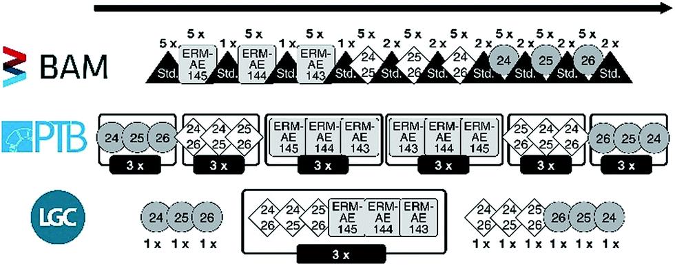
Since three sets of calibration solutions exist (labelled with the suffixes “-1b”, “-2b” and “-3b”), which allow independent calibrations, each lab was responsible to conduct independent calibration sequences using each of those three setups. The laboratories were also independently responsible for data treatment up to the point where each experimental sequence was fully described in terms of isotope signal ratios for the isotope ratios n(25Mg)/n(24Mg) and n(26Mg)/n(24Mg) for each of the components of the measurement: (a) each of the three calibration mixtures in the set used “24” + “25”, “24” + “26” and “25” + “26”, (b) the enriched materials “24Mg”, “25Mg” and “26Mg” and (c) the three IRM candidates; those values were to be associated with the standard uncertainties of the measurements based on the intra-sequence scatter of data on which the ratio (“R value”) is based. Those ratios were then evaluated to obtain the calibration factors, and the isotopic composition of the candidates from those.
Pre-tests have shown that:
(1) After measurement of a Mg sample (≈1 mg kg−1), the blank level was reached within 50 s of rinse time; total rinsing time between the sample and subsequent blank was 315 s.
(2) Interferences due to the formation of Mg hydrides in the plasma torch are insignificant; this has been verified by introducing a 26Mg enriched solution (≈1 mg kg−1) and detecting the signal of a potential 26Mg1H+ at m/z = 27, which was always at the blank level of 27Al. The mean hydride formation calculated from 3 measurements is <4 × 10⁻⁶; using the highest intensity measured for a single run as a worst case scenario, the formation is still <1 × 10⁻⁵ and thus negligible in this case.
In addition, also the whole sequence (Fig. 2) has been run as a pre-test to optimize its setup:
 | ||
| Fig. 2 Measurement sequence setups of the three partner laboratories. | ||
(1) The sequence started with a rinse cycle.
(2) Followed by a blank measurement.
(3) And finally, the sample.
(4) After each sample, the system was rinsed again, followed by the next blank measurement.
(5) Each sample was measured five times, only interrupted by rinse and blank measurements.
The pre-test sequences have specifically shown that:
(1) Blank intensity has been found to increase significantly during the sequence, particularly when an isotopically enriched material is introduced. This is shown in Fig. 3 for the 24Mg signal over the course of an actual measurement sequence.
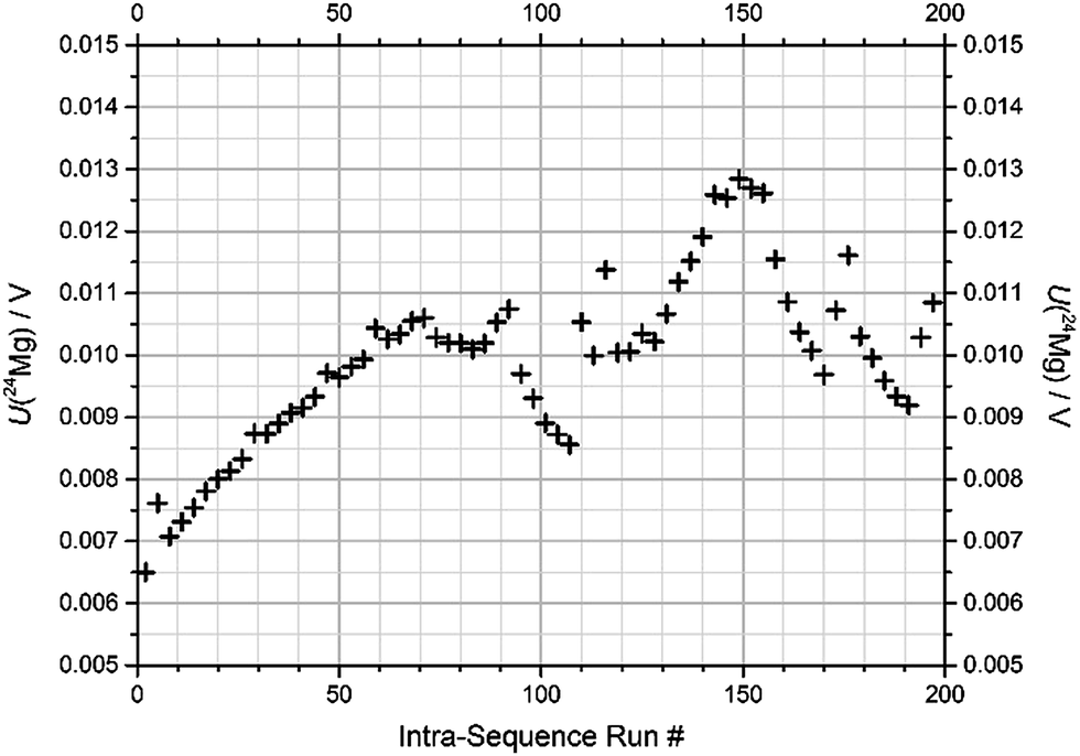 | ||
| Fig. 3 Blank values for 24Mg over the course of the described sequence (sequence “1b-3”, BAM). | ||
(2) Even after blank correction, the measured isotope ratios exhibit a significant drift over the course of the sequence, typically 0.022‰ per hour (Fig. 4 and Table 2).
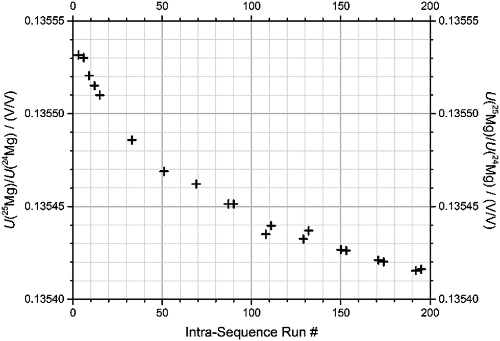 | ||
| Fig. 4 Drift of signal ratio U(25Mg)/U(24Mg) after blank-corrections, measured for an identical drift standard sample over the course of the described sequence (sequence “1b-3”, BAM). | ||
As a consequence of the blank build-up, the actual measurement sequences were set up such that they start from materials with a natural isotopic composition, moving to the three calibration mixtures with isotope ratios close to 1, and then finally end with the three isotopically enriched materials with isotope ratios >50.
To allow correction for the drift in the mass discrimination, a standard prepared from a natural magnesium sample was measured before and after each block of five identical samples; also, this standard was measured five times at the beginning of the sequence to establish a reference value for normalization.
The result of all pre-tests is a sequence with the following basic structure (Fig. 2):
(1) Measure the drift standard 5 times.
(2) Measure the three candidates, each in a block of 5 individual measurements, with one measurement of the drift standard in between those blocks; sequence of blocks: ERM-AE145, ERM-AE144, and ERM-AE143.
(3) Measure the three calibration solutions, each in a block of 5 individual measurements, with two measurements of the drift standard in between those blocks; sequence “24” + “25”, “25” + “26”, and “24” + “26”.
(4) Measure the three enriched starting materials, each in a block of 5 individual measurements, with two measurements of the drift standard in between those blocks; sequence “24Mg”, “25Mg”, and ”26Mg”.
(5) Drift standard again.
(6) Cleaning cycles (rinsing step of ≈1 h).
This sequence consists of 199 individual runs in total and takes about 14 h to complete. After each sequence, the system was rinsed. Nevertheless, the first blank for 24Mg of each sequence increased from below 1 mV before the first sequence to 7 mV in the last sequence. Fig. 3 shows the development of the 24Mg blank intensity over the course of the actual sequence “1b-3” at BAM. It is apparent that the blank value first increases due to the contact of the system with natural Mg with a mass fraction of 1 mg kg−1.
As soon as enriched materials are introduced, the blank is affected pronouncedly; the first solution, “24” + “25” (run #72), which actually has a lower 24Mg abundance than natural Mg, causes a drop in the 24Mg blank; this mixture is followed by two measurements of the natural Mg drift standard (run #87 and 90), which makes the blank value return to previous levels. The next mixture, “25” + “26” (starting at run #93), contains only trace amounts of 24Mg, and thus actually lets the 24Mg level drop almost towards its initial value; but the levels return with the measurement of the next drift standard (run #108 and 111). Then, when solution “24” + “26” is admitted (first at run #114), the blank drops again slightly – again because this binary mixture actually contains less 24Mg than natural Mg. After the following drift standard (#129 and 132), the solution of the enriched “24Mg” material is admitted (run #135) leading to an increase in the 24Mg blank. The following two drift standards (run #150 and 153) bring the 24Mg blank down a bit, which further proceeds with the enriched materials “25Mg” and “26Mg”. The measurement of drift standards in between (run #171 and 174) always leads to an increase of the blank levels. Note that each effect in the blank development which is visible for a specific run number is caused by a sample whose run number always is lower by 2.
Fig. 4 shows the signal ratio of U(25Mg)/U(24Mg), measured from the drift standard, again for the same sequence (“1b-3”) that was already discussed in the previous description of the blank values. Note that the values shown are based on outlier-corrected data, and after blank correction. The resulting drift in the measured isotope ratio shows a drift in the instrumental mass discrimination, which presumably is due to the drift in the ambient conditions of the MC-ICPMS (drift in temperature, exhaust flow, etc.). The drift shown in Fig. 4 is one of the largest, but also one of the steadiest drifts we have observed. All raw data have been corrected for their sequence specific drifts using the drift standard measurements, and normalizing to the five measurements of the drift standard was performed in the beginning of each sequence (run #3, 6, 9, 12, and 15).
Data preparation. For evaluation, all those data must be transferred into a set of signal ratios and standard uncertainties, which can be directly fed into the evaluation equations; all other corrections (blank corrections and drift normalizations) must have been applied before. At BAM, we have corrected the raw data in the following way, and obtained the required ratios as follows:
(1) Raw data were corrected for outliers (based on 2× standard deviation); this typically deletes a number of individual cycles measured for each sample (each run). Each sample was measured with 50 cycles, and outlier corrections typically removed 0 to 8 cycles per run.
(2) The outlier-corrected data for the blank measurements are collected, and the blank values before and after each sample run are averaged. Since those blanks were always measured right before and right after each sample run (with only the rinse cycle in between sample and blank), the averaged blank values are considered a good measure for the blank at the time of the sample measurement (no further interpolations were done for this correction). Those average values for the preceding and following blank are then subtracted from each individual measurement cycle of the sample run; finally, another outlier test is conducted with the blank-corrected data, and the resulting averages and standard deviations are collected as the blank-corrected values for the run. Signal ratios are calculated from those values; all the following evaluations occur only based on the signal ratios; absolute signals are not considered further.
(3) For each sample (all measured in a sequence), there exists one measurement of a drift standard right before and right after the block of sample runs. Those two measurements of the drift standard are collected. Since a number of sample runs (5 sample runs) lie in between the preceding and following drift standard measurements, and the individual run (that is to be corrected) is not necessarily in the centre between the two drift standard measurements; the drift standard was explicitly interpolated from the two adjacent measurements individually for each sample run. Then, the sample's values for the measured signal ratios were multiplied with the respective value of the drift standard (as measured at the beginning of the overall sequence, five times; this is the standard value for the drift normalization), and then this product was divided by the linearly interpolated (local) drift standard, which leads to normalization, and thereby removal of the drift.
(4) The drift-corrected signal ratios of the five runs per sample are collected; average values are calculated; standard uncertainties are calculated according to eqn (1).17,18
(5) The averages and standard uncertainties are collected into a table of experimental result values, which are fed into the evaluation.
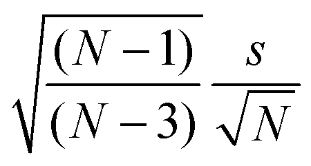 | (1) |
In the ESI, Table S2† shows values for the signal intensities and signal ratios after blank correction for the test sequence (sequence “1b-3”, BAM). Table S3 (ESI†) shows the signal ratios after drift correction of the data contained in Table S2 (ESI†).
Finally, Table 5 compiles the averages and standard uncertainties for the data compiled in Table S3 (ESI†); these data are later used in the evaluation (see Section 3.4) to determine the K-factors, which were used to evaluate the isotopic composition of the IRM candidates based on those data in Section 3.4.
| Sample | Experimental signal ratios and standard uncertainties | |||
|---|---|---|---|---|
| R(25/24)/(V/V) | u(R(25/24))/(V/V) | R(26/24)/(V/V) | u(R(26/24))/(V/V) | |
| a Candidate reference materials. | ||||
| ERM-AE145a | 0.1355428 | 0.0000011 | 0.1593391 | 0.0000010 |
| ERM-AE144a | 0.13552057 | 0.00000067 | 0.15929665 | 0.00000085 |
| ERM-AE143a | 0.1356328 | 0.0000020 | 0.1595551 | 0.0000028 |
| “24” + “25”-1b | 1.010347 | 0.000020 | 0.00371989 | 0.0000036 |
| “25” + “26”-1b | 46.4490 | 0.0043 | 51.2936 | 0.0048 |
| “24” + “26”-1b | 0.0022720 | 0.0000011 | 1.023272 | 0.000019 |
| “24Mg” | 0.0008418 | 0.0000015 | 0.0007537 | 0.0000018 |
| “25Mg” | 57.0117 | 0.0074 | 0.168842 | 0.000018 |
| “26Mg” | 0.38688 | 0.00025 | 274.36 | 0.15 |
(1) Measure the three isotopically enriched materials (“24Mg”, “25Mg”, and “26Mg”) one after another and repeat this sequence twice, which results in three individual measurements for each isotopically enriched material.
(2) Measure the three calibration solutions (“26Mg” + “24Mg”, “25Mg” + “24Mg”, and “25Mg” + “26Mg”) one after another and repeat this sequence twice, which also results in three individual measurements for each calibration solution.
(3) Measure the three candidates (ERM-AE145, ERM-AE144, and ERM-AE143), one after another and repeat this sequence twice.
(4) Then, repeat the measurement of the three candidates three times in reversed order (ERM-AE143, ERM-AE144, and ERM-AE145), which results in six individual measurements for each candidate.
(5) Measure the three calibration solutions again three times in reversed order (“25Mg” + “26Mg”, “25Mg” + “24Mg”, and “26Mg” + “24Mg”), which gives in sum six individual measurements for each calibration solution.
(6) Finally, measure the three isotopically enriched materials again three times in reversed order (“26Mg”, “25Mg”, and “24Mg”), which also gives in sum six individual measurements for each isotopically enriched material.
This kind of sequence consists of 109 individual measurements in total and takes about 21 h. During the sequence the blank shows variations in the intensities for 24Mg, 25Mg, and 26Mg. 24Mg increases from a minimum value of 0.08 mV to a maximum of 8 mV, 25Mg increases from a minimum of 0.02 mV to a maximum of 5 mV, and 26Mg increases from a minimum of 0.2 mV to 5 mV. Although the average blank intensity of 24Mg is higher than that of 25Mg and 26Mg, 25Mg and 26Mg are much more influenced by a high background, as the samples show a much lower natural abundance in these isotopes.
An internal drift correction was applied by step-wise normalization of repeated measurements and combining these normalized data in a quadratic polynomial covering the whole sequence, this way making use of the complete dataset without the need to include additional (time-consuming) measurements of a drift-standard.
Mg isotope ratio measurements can be affected by background spectral interferences originating from hydrogen, carbon, nitrogen and oxygen. These interferences are shown in Table 4. As seen from this table, doubly charged ions of magnesium combined with carbon can form spectral interferences on all Mg isotopes.
In order to ensure interference-free measurements we have opted for a strategy which involves measurements using the so-called cool plasma conditions, i.e., measurements with RF power setting set at lower values than those normally used. Measurement under cool plasma conditions is a known means of reducing the formation of doubly charged ions due to the fact that temperature of the plasma is somewhat lowered. Choi et al.19 studied background interferences at m/z of 24, 25 and 26, originating from hydrogen, carbon, nitrogen and oxygen – the elements with high ionisation potential – and found that their relative contributions to signals of Mg isotopes were lower in MC-ICPMS measurements under cool plasma conditions.
A criterion of interference-free measurements of Mg isotope ratios can be an agreement between theoretical and experimentally obtained slopes in a plot of δ′25/24Mg versus δ′26/24Mg, constructed according to the approach described in ref. 20–22.
In test measurements, we measured Mg isotope ratios of the LGC in-house Mg concentration standard and the IRMM-009 reference material relative to each other using a RF power of 950 W and 1150 W, without changing other instrumental parameters. Weighted linear regressions through the data points yielded a slope of 0.5173 ± 0.0038 for Mg isotope ratio measurements under a RF power of 950 W and a slope of 0.5224 ± 0.0018 for the measurements under a RF power of 1150 W (Fig. 5). It is worth noting that linear regression through the dataset comprising lesser data points, namely the data points of the LGC in-house standard relative to the IRMM-009 standard, yielded very similar figures with a slightly larger uncertainty of 0.5232 ± 0.0037 and 0.518 ± 0.008 for the measurements under hot and cool plasma, respectively. Theoretical slopes expected for mass fractionation in a plot of δ′25/24Mg vs. δ′26/24Mg are 0.5110 and 0.5210 for kinetic and equilibrium mass dependent fractionation, respectively, with uncertainties in the range of 10−7. As seen from these data, although Mg isotope ratio measurements both under cool and normal plasma conditions return slopes which agree with theoretical mass fractionation values within an uncertainty range, it is the measurements under cool plasma conditions that are characterised by a better match with the above criterion of interference-free measurements.
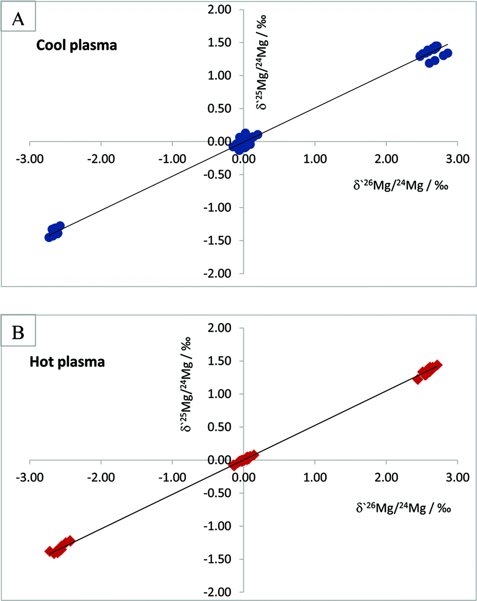 | ||
| Fig. 5 Three-isotope plots of Mg isotope ratio measurements by MC-ICPMS under cool plasma, RF power of 950 W (section A) and under hot plasma, RF power of 1150 W conditions (section B). See the text for details. | ||
3.4 Determination of K-factors and uncertainty budget
| Isotope | Atomic mass/u | Expanded uncertainty/u | k | Ref. |
|---|---|---|---|---|
| a Recommended values published by IUPAC 2003 (ref. 16) and in Metrologia26 based on the AME1995. b CRC Handbook of Chemistry and Physics.25 c IUPAC CIAAW 2012 recommended values27 based on ref. 24. d Atomic mass evaluation 2012.24 | ||||
| 24Mg | 23.98504187 | 0.00000026 | 6 | |
| 23.98504190 | 0.00000020 | 1 | ||
| 23.98504170 | 0.00000009 | 6 | ||
| 23.985041698 | 0.000000014 | 1 | ||
| 25Mg | 24.98583700 | 0.00000026 | 6 | |
| 24.98583702 | 0.00000020 | 1 | ||
| 24.9858370 | 0.0000003 | 6 | ||
| 24.98583698 | 0.00000005 | 1 | ||
| 26Mg | 25.98259300 | 0.00000026 | 6 | |
| 25.98259304 | 0.00000021 | 1 | ||
| 25.9825930 | 0.0000002 | 6 | ||
| 25.98259297 | 0.00000003 | 1 | ||
It is obvious that the atomic masses, which actually are relative atomic mass numbers, do only change in the 7th or 8th decimal place from 1995 to 2012. The Commission on Isotopic Abundances and Atomic Weights (CIAAW) of the International Union of Pure and Applied Chemistry (IUPAC) adopts the regularly published AME data, while enlarging the expanded uncertainty by using a coverage factor of k = 6 and recommends the resulting data for further use in isotope analysis. The AME 2012 data, printed in bold letters in Table 6, are currently the most recent and most precise data and therefore are used within this project. According to the currently valid definitions of the International Systems of Units (SI), the molar mass of a particle X is obtained from its relative atomic mass Ar(X) by the following equation:28
| M(X) = Ar(X)Mu | (2) |
 | (3) |
The atomic weights of all elements are regularly reviewed by the Commission on Isotope Abundances and Atomic Weights (CIAAW) of the International Union of Pure and Applied Chemistry (IUPAC).29 The published work on absolute isotope ratio measurements is assessed for each element and from this the so-called best measurements in a single terrestrial source and the standard atomic weight of the elements are selected and calculated. In the case of Mg, no standard atomic weight is provided anymore, but an interval, in order “to emphasize the fact that the atomic weight of Mg is not a constant of nature, but depends on the source of the material”.30 This is caused by the natural isotopic variations which are large enough that a substantial part of the terrestrial samples are outside the uncertainty interval of the previous standard atomic weight. Therefore, the atomic weight of Mg has to be selected from the diagram showing the Site-specific Natural Isotope Fractionation (SNIF diagram)30 depending on the nature of the material or it has to be determined, when more accurate data are required. The resulting atomic weight of Mg can be converted into the molar mass as described above by applying eqn (2).
 | (4) |
The amount-of-substance fractions result from the isotope ratios Ri as described in eqn (5):
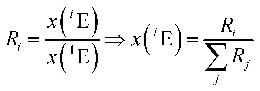 | (5) |
In the case of magnesium (meaning of indices: 1 = 24Mg, 2 = 25Mg, and 3 = 26Mg) eqn (4) and (5) can be combined to yield eqn (6):
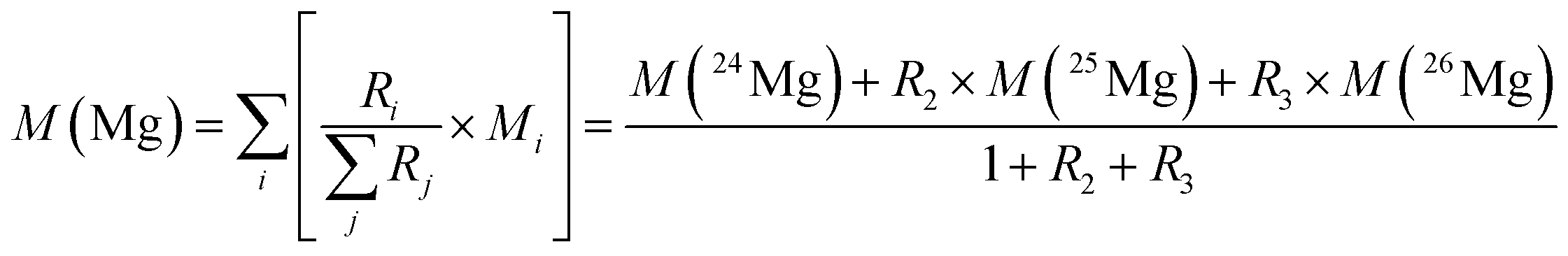 | (6) |
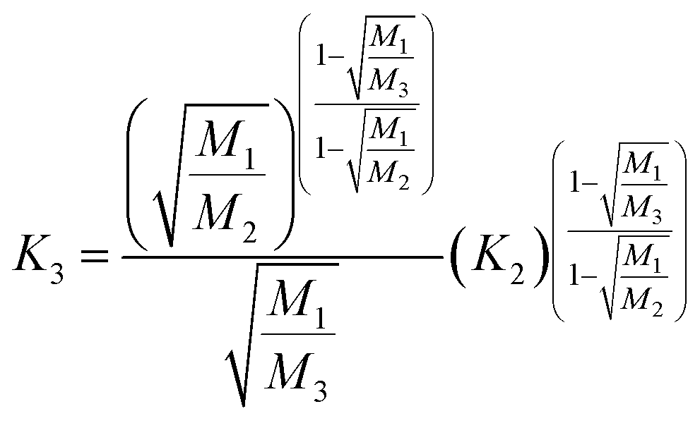
In eqn (6), the isotope ratios R2 and R3 have the following meanings and have to be calculated from the respective measured intensity (voltage) ratios Ui/U1 and the calibration factors K2 and K3:
 | (7) |
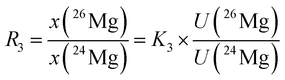 | (8) |
The calibration factors K2 and K3 were determined via the gravimetrically prepared synthetic isotope mixtures.4 The according analytical and numerical solutions are described in detail in ESI section S3.†
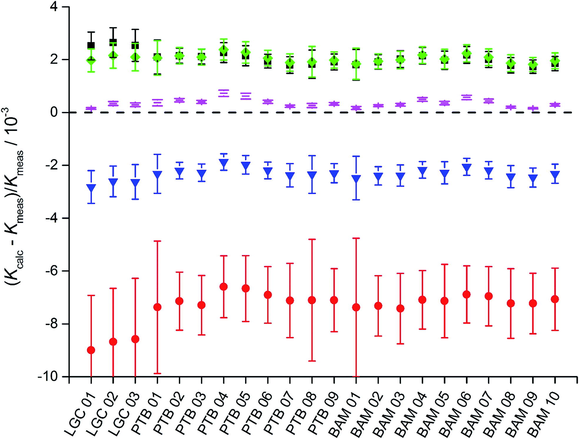
In short, from the six biased intensity ratios measured in the parent materials and at least one ratio from each of the two binary isotope mixtures plus the respective masses, the calibration factors K can be calculated straightforward. Since the set of equations describing the experimental approach with three parent materials A, B, and C and the three binary mixtures AB, AC, and BC is mathematically over-determined, twelve completely equivalent solutions are available (see ESI, Section S3†). Due to tiny experimental imperfections, these mathematical solutions yield slightly different results. Fig. 6a and b show typical calibration factors from the second out of nine measurement sequences performed at PTB.
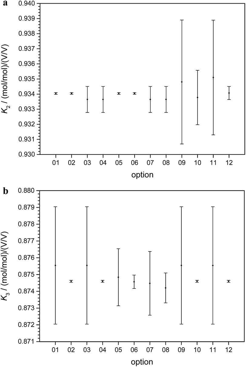 | ||
| Fig. 6 (a) Typical values and associated uncertainties (k = 2) for the 12 solutions (options) available for the calculation of the calibration factor K2 (25Mg/24Mg), based on the second out of nine measurement sequences performed at PTB. (b) Typical values and associated uncertainties (k = 2) for the 12 solutions (options) available for the calculation of the calibration factor K3 (26Mg/24Mg), based on the second out of nine measurement sequences performed at PTB. | ||
All results are consistent (not significantly different) within their associated uncertainties. Therefore, they have to be considered as equal within the limits of their uncertainties. For this reason, a single option can be selected arbitrarily. The most reasonable option is the one with the lowest uncertainty and therefore the highest reliability. In the case of K2 (Fig. 6a), options 01, 02, 05, and 06 seem to be the most promising choices.
In the case of K3 (Fig. 6b), the options 02, 04, 10, and 12 exhibit the smallest uncertainties. Therefore, 02 as the only option with small uncertainties associated with both K2 and K3 was chosen. This result does not come as a surprise, because option 02 relies on the intensity ratio 25Mg/24Mg in the mixture AB prepared from “25Mg” and “24Mg” and on the intensity ratio 26Mg/24Mg in the mixture AC prepared from “26Mg” and “24Mg”. Both mixtures were prepared in a way to adjust these two ratios close to unity with all the beneficial impact on the uncertainties associated with the intensity ratios. The comprehensive uncertainty analysis has identified these two ratios as the most important input quantities (with comparatively large sensitivity coefficients), which is the reason why option 02 yields the smallest overall uncertainty. The analytical and the numerical solutions yield exactly the same results and (at least in this case of excellent convergence) also exactly the same associated uncertainties. The analytical solution has the advantage of more compact calculations (especially in the case of the uncertainty estimation) and the SI traceability of the result can be claimed and demonstrated easier from the single equation than from the recursive algorithms.
3.5 Characterization of IRM candidates
The whole setup was designed such that each set of solutions contains a full set of calibration solutions and a full set of candidate materials as well. Thus, each measurement sequence conducted at each of the partner laboratories on a full set of solutions yielded independent results for the candidate materials (see Section 3.3). Those results for one sequence (BAM, third sequence measured using calibration solutions “24” + “25”-1b, “24” + “26”-1b and “25” + “26”-1b) are exemplarily listed in Table 7. All such data for all sequences measured in all laboratories are compiled in Tables S7 to S9 in the ESI.† The values from these tables in the ESI are shown in Fig. 7. All those resources (Tables 7 and S7 to S9 in the ESI,† and Fig. 7) contain the expanded uncertainties for all data (k = 2), which are based on evaluations of the full uncertainty budgets using the GUM Workbench for each sequence.| Parameter | Unit | Candidate ERM-AE143 | Candidate ERM-AE144 | Candidate ERM-AE145 |
|---|---|---|---|---|
| Isotope amount fractions | ||||
| x(24Mg) | mol mol−1 | 0.789880(11) | 0.790087(10) | 0.790051(10) |
| x(25Mg) | mol mol−1 | 0.1000066(72) | 0.0999500(67) | 0.0999618(69) |
| x(26Mg) | mol mol−1 | 0.1101129(83) | 0.1099633(76) | 0.1099875(76) |
|
||||
| Isotope amount ratios | ||||
| R(25Mg/24Mg) | mol mol−1 | 0.126610(10) | 0.1265050(97) | 0.1265258(99) |
| R(26Mg/24Mg) | mol mol−1 | 0.139405(12) | 0.139179(11) | 0.139216(11) |
|
||||
| Atomic weights | ||||
| A r(Mg) | 24.305084(18) | 24.304728(17) | 24.304789(17) | |
 | ||
| Fig. 7 All measurement results for the three IRM candidates from all three laboratories. All graphs in one row have identical axis scaling. | ||
4. Discussion
4.1 Final results for the three candidate materials
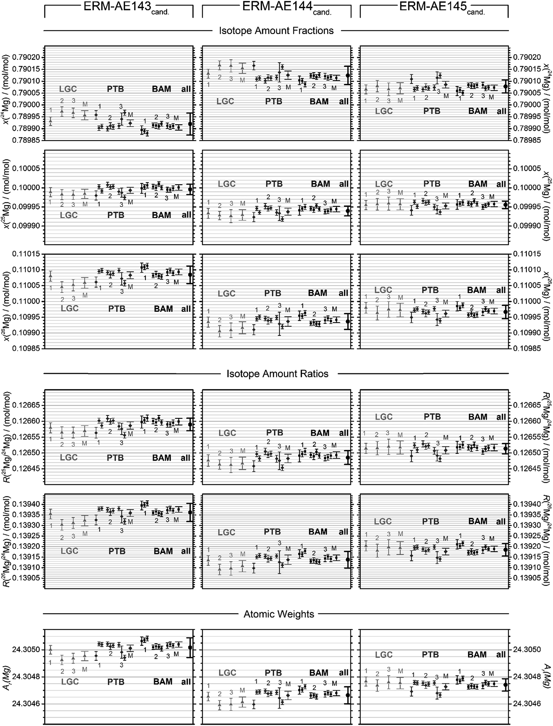
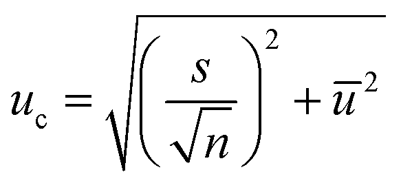
The final values (Fig. 7 and Table 8) for each quantity are obtained by calculating the arithmetic mean not from the laboratory means but from the individual results for each measured sequence (Fig. 7). The associated measurement uncertainties are calculated as the mean of the individual measurement uncertainties (eqn (9)) plus the standard deviation of the mean of all individual results (eqn (10)).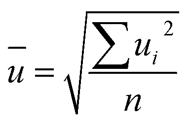 | (9) |
 | (10) |
 | (11) |
| Parameter | Unit | Candidate ERM-AE143 | Candidate ERM-AE144 | Candidate ERM-AE145 |
|---|---|---|---|---|
| Isotope amount fractions | ||||
| x(24Mg) | mol mol−1 | 0.789920(46) | 0.790124(39) | 0.790078(28) |
| x(25Mg) | mol mol−1 | 0.099996(14) | 0.099939(13) | 0.099956(10) |
| x(26Mg) | mol mol−1 | 0.110085(28) | 0.109936(25) | 0.109967(21) |
|
||||
| Isotope amount ratios | ||||
| R(25Mg/24Mg) | mol mol−1 | 0.126590(20) | 0.126486(22) | 0.126514(16) |
| R(26Mg/24Mg) | mol mol−1 | 0.139362(43) | 0.139138(39) | 0.139185(29) |
|
||||
| Atomic weights | ||||
| A r(Mg) | 24.305017(73) | 24.304664(63) | 24.304741(46) | |
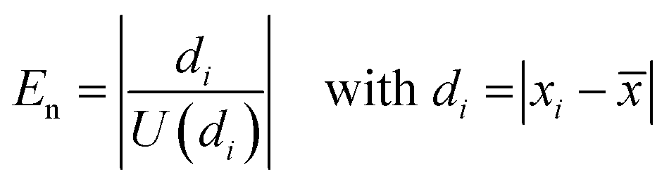
However, it turned out that between 1 and 7 individual results are metrologically not compatible with the mean value, which means that their normalized error, En (eqn (11)), is larger than 1. The conclusion is that either the uncertainties of the individual results or the uncertainty of the mean value, or both are underestimated. Reasons for that might be that the measured isotope ratios contain some assumptions based on separate measurements such as the blank correction or the absence of interferences. Although these measurement based assumptions nearly reflect the real conditions, there might be some cases where a tiny underestimation occurs, which gets visible when working with relative measurement uncertainties at the 0.005% level.
Based on the work by Kessel et al. we added an additional uncertainty contribution in order to establish the metrological compatibility of the results.31 As the uncertainties of the individual results are carefully calculated and the agreement of the individual results is rather good (although not perfect), we added the additional uncertainty contribution to the mean value and not to the individual values. This additional uncertainty contribution was estimated such that 95% (21) of the 22 individual results show normalized errors equal to or less than 1. For the n(25Mg)/n(24Mg) ratios, the additional uncertainty contribution typically is equal to or less than the combined standard uncertainty of the mean value. In the case of the n(26Mg)/n(24Mg) ratio, the additional uncertainty contribution ranges between the one- and twofold of the combined standard uncertainty of the mean value. This is in agreement with the fact that the n(26Mg)/n(24Mg) ratio measurement is more severely impeded by mass discrimination and by potential molecular interferences compared to the n(25Mg)/n(24Mg) ratio measurement.
The isotopic compositions of all three candidate materials (Table 8) are within the natural isotope variation.30 All three materials show isotopic compositions which are close together with a maximum spread of 1.6‰ for the n(26Mg)/n(24Mg) ratio. Candidate ERM-AE143 is isotopically heavier, i.e. higher atomic weight, than ERM-AE145 and ERM-AE144 with ERM-AE144 showing the lowest atomic weight. Usually, one might expect the atomic weight of ERM-AE145 to be lower than that of ERM-AE144, from which it is prepared by HV-sublimation typically leading to a lighter isotopic composition due to isotopic fractionation, but actually it is the other way round. The reason is that in the beginning of the sublimation process the first and lightest Mg fraction escapes through the hole in the glassy carbon lid and condenses at the copper cooling block above (for details on the sublimation apparatus see ref. 4). Therefore, the lightest Mg fraction is lost, while all subsequent fractions being heavier in their isotopic composition are condensed at the glassy carbon lid. Considering a nearly quantitative recovery, it is obvious that the collected sublimate Mg is isotopically heavier than the starting material.
| Parameter | Unit | White and Cameron38natural Mg | Catanzaro et al.39 NIST SRM 980 | Bizzarro et al.40 J12 olivine | This work ERM-AE143 |
|---|---|---|---|---|---|
| Isotope amount fraction | |||||
| x(24Mg) | mol mol−1 | 0.7860(79) | 0.78992(25) | 0.789548(26) | 0.789920(46) |
| x(25Mg) | mol mol−1 | 0.1011(10) | 0.10003(9) | 0.100190(18) | 0.099996(14) |
| x(26Mg) | mol mol−1 | 0.1129(11) | 0.11005(19) | 0.110261(23) | 0.110085(28) |
|
|||||
| Isotope amount ratio | |||||
| R(25Mg/24Mg) | mol mol−1 | Not provided | 0.12663(13) | 0.126896(25) | 0.126590(20) |
| R(26Mg/24Mg) | mol mol−1 | Not provided | 0.13932(26) | 0.139652(33) | 0.139362(43) |
|
|||||
| Atomic weight | |||||
| A r(Mg) | 24.31 | 24.30497(44) | 24.305565(45) | 24.305017(73) | |
The relative expanded uncertainties for the isotope amount ratios in the three candidate materials range from 0.013% to 0.017% for the n(25Mg)/n(24Mg) ratio and from 0.021% to 0.031% for the n(26Mg)/n(24Mg) ratio. For the isotope amount fractions x(24Mg), x(25Mg) and x(26Mg), the relative expanded uncertainties are 0.006%, ≤0.015% and ≤0.025%, respectively.
For the case of the atomic weights the relative expanded uncertainties are ≤0.0003%. Thus the project's target uncertainty of 0.05% for the isotope amount ratios has been underrun at least by a factor of 2. Moreover, the standard uncertainty for the isotope amount ratios is at the same level (≈0.1‰) as the precision of delta measurements observed for standard measurements and reported from geochemical applications.32,33 To the knowledge of the authors this is the first time that absolute isotope ratios, i.e. isotope amount ratios, were determined with associated standard uncertainties being at the same level as the precision of delta measurements reported as 2sd.
The most important contributions to the uncertainty associated with the isotope amount ratios n(25Mg)/n(24Mg) and n(26Mg)/n(24Mg) determined in an individual measurement sequence are displayed in Fig. 8. It is obvious that nearly two thirds of the measurement uncertainty is due to the uncertainty contributions from the masses of the isotopically enriched Mg materials in the calibration mixtures, which were introduced during the preparation of the calibration solutions in the first part of the project. These contributions themselves are dominated by the uncertainty contributions of the weighing and of the purity statement.4 The third largest contribution is the measured intensity ratio in the calibration mixture and only in the fourth place comes the measured intensity ratio of the candidate material. This clearly shows that a reduction of the final uncertainty is only possible, when the weighing procedure and the purity assessment are improved. An improvement of the ion intensity ratio measurement is only of secondary importance.
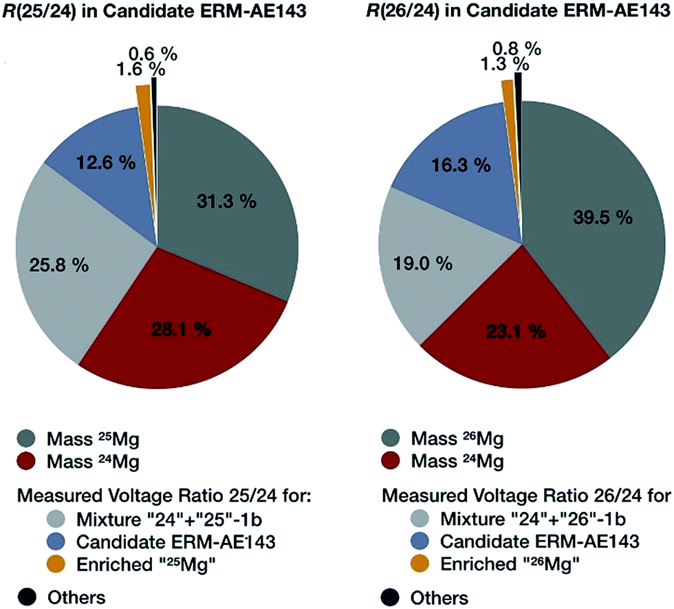 | ||
| Fig. 8 Most important contributions to the uncertainties of the two magnesium isotope ratios determined in an individual measurement sequence (Mg-1b-3, BAM) for candidate ERM-AE143 as the example. | ||
It has to be noted here that the measurement uncertainty represented in Fig. 8 is not the final uncertainty; it is the uncertainty of one out of 22 individual measurement sequences, which are combined to result in the final value. The expanded measurement uncertainties in Fig. 7 are 0.000010 mol mol−1 for n(25Mg)/n(24Mg) and 0.000012 mol mol−1 for n(26Mg)/n(24Mg), which are increased by a factor between 1.4 and 1.7 when all individual results are combined (Table 8).
4.2 Choice of the material for IRM
Candidate ERM-AE143 offers an atomic weight very close to the certified value of NIST SRM 980; both atomic weights agree within their limits of uncertainty. This close agreement in the isotopic composition makes ERM-AE143 well suited as a replacement material of NIST SRM 980. Additionally, the raw material is excellently characterized concerning its purity. Consequently, candidate ERM-AE143 is selected as the new primary isotopic reference material and as a new anchor point of the δ26/24Mg scale representing the zero-point. The candidates ERM-AE144 and -AE145 show slightly lower atomic weights and offer theoretical δ26/24MgERM-AE143-values of approximately −1.6‰ and −1.3‰, respectively. This makes them perfectly suited as additional materials for defining the negative δ-scale. The candidates ERM-AE144 and -AE145 are of course also primary isotopic reference materials concerning the absolute isotopic composition, as their quality is at the same level as that of candidate ERM-AE143. However, in δ-scale measurements only one material can be used as the anchor point of the scale.34 The candidates ERM-AE144 and -AE145 will serve as primary materials defining the scale span. The three materials will become available in 2016/2017 via BAM.For this it is necessary to replace the theoretical delta values by measured delta values, which will be carried out in an upcoming project.
4.3 Considerations on the mass discrimination coefficient and the validity of fractionation laws
Fractionation laws are often used to correct (instrumental) mass fractionation/discrimination of one isotope ratio of an element via the determined mass fractionation of a second isotope ratio of the same element either for absolute isotope ratios, relative isotope ratios or radiogenic isotope ratios.The current dataset, which provides to our knowledge the most accurate (smallest uncertainties) absolute isotope ratios measured for Mg, allows us to test the validity of the above described assumptions for MC-ICPMS. The K-factor K2-02 (25Mg/24Mg) was chosen as the input quantity, which was used to calculate the K-factor for the 26Mg/24Mg ratio. Finally, the deviation of the K-factor obtained via fractionation laws was calculated from the K-factor K3-02 (26Mg/24Mg) obtained from the synthetic isotope mixtures for all measured sequences (Table S10, ESI†). These calculations were carried out for the five fractionation laws available in the literature (eqn (12) to (16) (ref. 8, 35 and 36)).
Linear law 1 (Taylor et al.35):
 | (12) |
Linear law 2 (Zindler and Hart36):
 | (13) |
Power law (Zindler and Hart36), power law (Taylor et al.35), and exponential law (Taylor et al.35):
 | (14) |
Rayleigh law (Zindler and Hart36):
 | (15) |
Exponential law (Zindler and Hart36) and Russel's law:37
 | (16) |
It has to be noted here that the exponential law and the power law presented in Taylor et al.35 are equivalent8,37 and can be converted into the power law published by Zindler and Hart;36 thus only the latter was used. The exponential law according to Zindler and Hart36 sometimes is denoted as Russel's law.37
Detailed information on the individual fractionation laws is given in the ESI in Section S5.†
The deviation of the so calculated K-factors obtained via fractionation laws from the K-factor K3-02 (26Mg/24Mg) obtained from the synthetic isotope mixtures is significant (Fig. 9 and Table S9, ESI†), especially when considering at which precision level isotope data currently are interpreted. The application of the linear law 1 results in a negative bias between −7‰ and −9‰, while the application of the linear law 2 results in a positive bias between +1.7‰ and +2.6‰. The power law causes a negative bias between −1.9‰ and −2.8‰, while the Rayleigh law causes a positive bias of the same extent between +1.8‰ and +2.4‰. Only the application of the exponential law is capable of producing a bias significantly below the 1‰ level (0.1‰ to 0.7‰). None of the applied fractionation laws yields a produced K-factor, which agrees with the reference value obtained from the synthetic isotope mixtures within the stated uncertainties. It has to be stressed here that these biases only apply for ICPMS measurements, but not necessarily other mass spectrometric techniques such as TIMS. And it is obvious that these fractionation laws do not accurately describe the mass discrimination of an ICPMS instrument, and therefore should not be used for isotope analysis unless conventional methods are applied, as is the case for e.g. radiogenic 87Sr/86Sr applications or delta measurements combined with the double-spike technique. Even in this case, the exponential law should be favoured over the others. In all cases, it has to be stated clearly which fractionation law has been applied and all necessary data should be provided to enable conversion calculations.
 | ||
| Fig. 9 Relative deviations of the K factors for the isotope ratio 26Mg/24Mg calculated from the K factor 25Mg/24Mg (determined experimentally via gravimetric mixtures) using the linear law 1 (red circle), the linear law 2 (black square), the power law (blue triangle), the Rayleigh law (green diamonds) and the exponential law (magenta line) from the reference value determined using the isotopic mixtures (dashed black line). While the linear law 1 and the power law show negative deviations from the reference, the linear law 2, the Rayleigh law and the exponential law cause positive deviations, with the exponential law showing the smallest absolute deviations. However, no calculated result equals the reference value. | ||
The observed bias for the different fractionation law is no evidence for mass-independent fractionation in the ICPMS instrument, especially as the bias decreases from the linear to the exponential law. Even after improving the mathematical relationship between the isotope mass and K-factor, there are still small, isotope-independent contributions present such as amplifier gain (although partially corrected for) and detector efficiency. The data presented here unfortunately cannot be used for refining the fractionation laws or setting up discrimination laws for ICPMS as Mg offers too few isotope ratios. However, precise and accurate data for Mg are now available for future considerations, which describe the mass discrimination for Mg in ICPMS and how good current fractionation laws model these effects.
4.4 Comparison with other measurements
Over the decades only very few measurements of absolute isotope ratios have been carried out, mainly caused by the huge workload. To date, only the studies of White and Cameron,38 Catanzaro et al.39 and Bizzarro et al.40 are known, which all have been rated as the best measurements by IUPAC, whereby the work of Bizzarro et al. represents the current best measurement.41 White and Cameron38 distilled Mg into the ion source where Mg vapour was ionized by electron impact. The mass spectrometer developed by A. O. C. Nier was not calibrated, as the measurements took place before Nier invented the calibration principle in 1950.5 Also mass fractionation was not corrected for but partially considered in the uncertainty of 1% for the isotope abundances (Table 9).At this time, 1948, this approach was quite reasonable, confirmed by the fact that the so obtained Mg atomic weight still agrees with later determinations when assuming an uncertainty of 1 in the fourth digit. In 1966, Catanzaro et al.39 performed the first calibrated measurement for Mg isotope ratios using 24Mg and 26Mg enriched materials for preparing the synthetic isotope mixtures and applying TIMS as the mass spectrometric technique. According to current IUPAC definitions, this cannot be considered a fully calibrated measurement, as only 2 out of 3 isotopes were calibrated. Catanzaro et al.39 obtained highly accurate results (Table 9), which on one hand confirmed the data obtained by White and Cameron38 and on the other hand provided a highly accurate atomic weight and isotopic composition of Mg for the next four decades.
As already discussed, upcoming heterogeneity issues of NIST SRM 980 made it necessary to provide new Mg isotope reference materials offering absolute Mg isotope ratios. In 2011, Bizzarro et al.40 published absolute Mg isotope ratios which have been obtained by using a 26Mg–24Mg double spike technique and multicollector ICPMS with a high mass resolution capability. These author's stated uncertainties are by a factor of 5 to 8 lower than those obtained by Catanzaro et al.39
As a consequence of the double-spike approach, Bizzarro et al.40 assumed that mass fractionation laws could describe the instrumental mass fractionation/mass discrimination and stated themselves that in the case this assumption would not hold true the 25Mg/24Mg ratio could in the worst case (kinetic fractionation process) be biased by up to 1‰; the 26Mg/24Mg would be not affected due to the direct calibration via the 26Mg–24Mg double spike.
In Section 4.3 it was shown that current fractionation laws cannot fully describe the mass fractionation/discrimination in an ICPMS; even the best approach shows a bias of approximately 0.4‰. Therefore, the absolute 25Mg/24Mg ratio provided by Bizzarro et al.40 and consequently the derived data (isotope amount fractions, atomic weight) are assumed to show a small although significant bias which is not covered by the uncertainty. Further issues supporting this statement have already been discussed in ref. 4.
The Mg atomic weight published by Bizzarro et al.40 represents a significantly heavier isotopic composition than those published by Catanzaro et al.39 (Table 9). Typically, high purity magnesium metals, such as those presumably used by Catanzaro et al.39 but also in this work, show lighter isotopic composition due to the purification process than mantle derived minerals such as the J12 olivine analysed by Bizzarro et al.40 Samples such as the J12 olivine, however, are important as well as they may serve as secondary standards for quality control, when properly characterized.
The data obtained in this work (Table 8 and 9) were fully calibrated by means of three synthetic isotope mixtures, which have been prepared from isotopically enriched materials “24Mg”, “25Mg” and “26Mg”, each featuring complete purity statements.4 No a priori assumptions have been made and therefore an ab initio calibration has been established.
Moreover, the synthetic isotope mixtures have been produced in three replicates and measurements have been carried out at three institutes by applying multicollector ICPMS. Therefore, real reproducibility (different laboratories) is included in the uncertainty budget confirming the independence of our results from place and time.
The atomic weight and the isotopic composition of Mg obtained in this work agree well with the data published by Catanzaro et al.39 and those published by White and Cameron.38 They do not agree with those published by Bizzarro et al.40 The obtained measurement uncertainties in this work are a factor of 6 lower than those obtained by Catanzaro et al.39 and are at the same level as those published by Bizzarro et al.,40 although it has to be noted that the uncertainty in this work already includes the reproducibility of different laboratories and different calibration mixtures.
5. Conclusions
Using the synthetic isotope mixtures prepared from isotopically enriched and purified Mg materials as described in ref. 4, three multicollector ICPMS instruments were fully calibrated. No a priori assumptions were made, all influencing quantities were determined. Applying this ab initio calibration the Mg isotopic compositions of three candidate isotopic reference materials were determined. A set of three candidate reference materials were characterized with candidate ERM-AE143 being nearly identical to NIST SRM 980 in terms of its Mg isotopic composition. The candidates ERM-AE144 and -AE145 are isotopically lighter than ERM-AE143 by approximately −1.6‰ and −1.3‰. Together with ERM-AE143 for the first time a set of Mg isotope reference materials will become available, which span a range of Mg isotope compositions of approximately 1.6‰.The combined uncertainties of a single measurement sequence are dominated by the weighing data and the purity statement of the isotopically enriched materials used for the synthetic isotope mixtures. When combining all individual measurement sequences, the reproducibility of the results contributes significantly and increases the overall uncertainty by a factor of ≤1.5 for the isotope ratio R(25Mg/24Mg) and by a factor of ≤2 for the isotope ratio R(26Mg/24Mg).
The final relative standard uncertainties are ≤0.1‰ for the isotope ratio R(25Mg/24Mg) and ≤0.16‰ for the isotope ratio R(26Mg/24Mg) and thus are at the level of current delta measurements. With these uncertainties, the project's target uncertainty of <0.5‰ (relative, k = 2) for the magnesium isotopic reference material has been achieved.
The measurement results presented in this work are superior in quality to the current best measurement as listed by IUPAC,41 because the mass spectrometers were fully calibrated and the reproducibility of the measurements was demonstrated. Furthermore, the current best measurement was obtained by a double-spike technique applying assumptions which are not valid for absolute isotope measurements as demonstrated in this work. Therefore, we advise to replace the current best measurement by the data presented in this work.
Although we could show that absolute isotope ratio measurements are possible at the precision level of today's routine delta measurements for Mg, it was a huge effort to achieve this aim. Nevertheless, further improvement is still necessary when moving to elements requiring higher precision of the delta measurements. In this context, improvements can only be made, when the weighing process and the purity assessment of the purified and isotopically enriched materials are improved. For elements whose stable isotopes are not completely available in enriched form, so that a full calibration would not be possible, new ways have to be found. The mass fractionation or mass discrimination of isotope ratios cannot be calculated by applying current fractionation laws, as we have also shown that such approaches are not sufficiently accurate.
Acknowledgements
Financial support by EMRP (the European Metrology Research Programme) is gratefully acknowledged (EMRP-SIB09 "Primary standards for challenging elements").12 The EMRP is jointly funded by the EMRP participating countries within EURAMET and the European Union. The authors explicitly thank Heinrich Kipphardt and Wolfgang Pritzkow for helpful advice and Maren Koenig, Dorit Becker, Ti Ha Le, Carola Pape, and Volker Görlitz for assistance with the preparative work.Notes and references
- S. Kelly, K. Heaton and J. Hoogewerff, Trends Food Sci. Technol., 2005, 16, 555 CrossRef CAS.
- A. Galy, E. Young, R. Ash and R. O'Nions, Science, 2000, 290, 1751 CrossRef CAS PubMed.
- B. Shen, J. Wimpenny, C.-T. Lee, D. Tollstrup and Q.-Z. Yin, Chem. Geol., 2013, 356, 209 CrossRef CAS.
- B. Brandt, J. Vogl, J. Noordmann, A. Kaltenbach and O. Rienitz, J. Anal. At. Spectrom., 2016, 31, 179 RSC.
- A. O. Nier, Phys. Rev., 1950, 77, 789 CrossRef CAS.
- T. Hirata and T. Ohno, J. Anal. At. Spectrom., 2001, 16, 487 RSC.
- A. Galy, O. Yoffe, P. E. Janney, R. W. Williams, C. Cloquet, O. Alard, O. L. Halicz, M. Wadhwa, I. D. Hutcheon, E. Rmon and J. Carignan, J. Anal. At. Spectrom., 2003, 18, 1352 RSC.
- W. Pritzkow, S. Wunderli, J. Vogl and G. Fortunato, Int. J. Mass Spectrom., 2007, 261, 74 CrossRef CAS.
- J. Vogl and M. Rosner, Geostand. Geoanal. Res., 2012, 36, 161 CrossRef CAS.
- Joint Committee for Guides in Metrology (JCGM/WG 1), “Evaluation of measurement data - Guide to the expression of uncertainty in measurement,” JCGM, 2008.
- Metrodata GmbH, GUM Workbench Pro 2.4.1.375, Weil am Rhein, 2009, http://www.metrodata.de/, accessed 24.03.2016.
- “Primary standards for challenging elements,” [Online]. Available: https://www.ptb.de/emrp/sib09.html, accessed 30.06.2015.
- “BAM Primary Pure Substances,” [Online]. Available: http://www.rm-certificates.bam.de/en/certificates/primary_pure_substances/index.htm, accessed 30.06.2015.
- G. Petzow, Metallographisches, Keramographische, Plastographisches Ätzen, 6, überarbeitete Auflage, Gebrüder Borntraeger Berlin - Stuttgart, Berlin, Stuttgart, 2006 Search PubMed.
- G. Mana and O. Rienitz, Int. J. Mass Spectrom., 2010, 291, 55 CrossRef CAS.
- J. De Laeter, J. Bohlke, P. De Bievre, H. Hidaka, H. Peiser, K. Rosman and P. Taylor, Pure Appl. Chem., 2003, 75, 683 CrossRef CAS.
- BIPM, JCGM 101:2008, Evaluation of measurement data - Supplement 1 to the “Guide to the expression of uncertainty in measurement” - Propagation of distributions using a Monte Carlo method, 1st edn, 2008.
- R. Kacker and A. Jones, Metrologia, 2003, 40, 235 CrossRef.
- M. S. Choi, J.-S. Ryu, S.-W. Lee, H. S. Shin and K. S. Lee, J. Anal. At. Spectrom., 2012, 27, 1955 RSC.
- E. Young, A. Galy and H. Nagahara, Geochim. Cosmochim. Acta, 2002, 66, 1095 CrossRef CAS.
- E. Young and A. Galy, Rev. Mineral. Geochem., 2004, 55, 197 CrossRef CAS.
- T. Walczyk, Anal. Bioanal. Chem., 2004, 378, 229 CrossRef CAS PubMed.
- G. Audi, M. Wang, A. Wapstra, F. Kondev, M. MacCormick, X. Xu and B. Pfeiffer, Chin. Phys. C, 2012, 36, 1287 CrossRef.
- M. Wang, G. Audi, A. A. H. Wapstra, F. Kondev, M. MacCormick, X. Xu and B. Pfeiffer, Chin. Phys. C, 2012, 36, 1603 CrossRef.
- D. R. Lide, CRC Handbook of Chemistry and Physics, ed. D. R. Lide, CRC Press LLC, Boca Raton, 82nd edn, 2001 Search PubMed.
- P. De Bievre and H. S. Peiser, Metrologia, 1997, 34, 49 CrossRef.
- “Commission on Isotopic Abundances and Atomic Weights - Atomic Masses,” [Online]: http://www.ciaaw.org/atomic-masses.htm, accessed 24.03.2016.
- P. Mohr, B. Taylor and D. Newell, J. Phys. Chem. Ref. Data, 2012, 41, 043109 CrossRef.
- “Commission on Isotope Abundances and Atomic Weights,” [Online]: http://www.ciaaw.org, accessed 24.03.2016.
- “Commission on Isotope Abundances and Atomic Weights - Magnesium,” [Online]: http://www.ciaaw.org/magnesium.htm, accessed 24.03.2016.
- R. Kessel, M. Berglund and R. Wellum, Accredit. Qual. Assur., 2008, 13, 293 CrossRef CAS.
- V. Chang, A. Makishima, N. Belshaw and R. O'Nions, J. Anal. At. Spectrom., 2003, 18, 296 RSC.
- F. Wombacher, A. Eisenhauer, A. Heuser and S. Weyer, J. Anal. At. Spectrom., 2009, 24, 627 RSC.
- W. Brand, T. Coplen, J. Vogl, M. Rosner and T. Prohaska, Pure Appl. Chem., 2014, 86, 425 CrossRef CAS.
- P. D. P Taylor, P. Debievre, A. J. Walder and A. Entwistle, J. Anal. At. Spectrom., 1995, 10, 395 RSC.
- S. R. Hart and A. Zindler, Int. J. Mass Spectrom. Ion Processes, 1989, 89, 287 CrossRef CAS.
- J. Meija, L. Yang, Z. Mester and R. Sturgeon, Correction of Instrumental Mass Discrimination for Isotope Ratio Determination with Multi-collector Inductively Coupled Plasma Mass Spectrometry, in Isotopic Analysis, Wiley-VCH Verlag & Co KGaA, Weinheim, 2012, pp. 113–138 Search PubMed.
- J. R. White and A. E. Cameron, Phys. Rev., 1948, 74, 991 CrossRef CAS.
- E. Catanzaro, T. Murphy, E. Garner and W. Shields, J. Res. Natl. Inst. Stand. Technol., 1966, 70A, 453 Search PubMed.
- M. Bizzarro, C. Paton, K. Larsen, M. Schiller, A. Trinquier and D. Ulfbeck, J. Anal. At. Spectrom., 2011, 26, 565 RSC.
- J. Meija, T. Coplen, M. Berglund, W. Brand, P. De Bievre, M. Groening, N. Holden, J. Irrgeher, R. Loss, T. Walczyk and T. Prohaska, Pure Appl. Chem., 2016, 88, 293 CAS.
Footnote |
| † Electronic supplementary information (ESI) available: Characterization of a new absolute isotope reference material for magnesium: calibration of the mass spectrometers, determination of isotopic compositions, and full uncertainty budget. See DOI: 10.1039/c6ja00013d |
| This journal is © The Royal Society of Chemistry 2016 |