 Open Access Article
 This Open Access Article is licensed under a
 Creative Commons Attribution 3.0 Unported Licence
Microcanonical and thermal instanton rate theory for chemical reactions at all temperatures
Jeremy O.
Richardson
 ab
ab
aDepartment of Chemistry, Durham University, South Road, Durham, DH1 3LE, UK
bLaboratory of Physical Chemistry, ETH Zurich, 8093 Zurich, Switzerland. E-mail: jeremy.richardson@phys.chem.ethz.ch
First published on 23rd May 2016
Abstract
Semiclassical instanton theory is used to study the quantum effects of tunnelling and delocalization in molecular systems. An analysis of the approximations involved in the method is presented based on a recent first-principles derivation of instanton rate theory [J. Chem. Phys., 2016, 144, 114106]. It is known that the standard instanton method is unable to accurately compute thermal rates near the crossover temperature. The causes of this problem are identified and an improved method is proposed, whereby an instanton approximation to the microcanonical rate is defined and integrated numerically to obtain a thermal rate at any temperature. No new computational algorithms are required, but only data analysis of a number of standard instanton calculations.
1 Introduction
Instanton theory provides a method which allows the computation of thermal rate constants of chemical reactions including the quantum-mechanical effects of tunnelling and zero-point energy. It is sometimes known as semiclassical transition-state theory (SCTST)1,2 as it provides an approximate quantum-mechanical generalization of classical transition-state theory. Instead of requiring knowledge only of the geometry at the top of the potential-energy barrier (the transition state), one locates a pathway which describes the dominant tunnelling pathway through the barrier.The theory has been used extensively in a wide range of applications in physics and chemistry based on “Im F” arguments.3–30 The author recently rederived the method from first principles, using semiclassical approximations to the exact expression for the rate.31 All these instanton approaches give equivalent results, however.32
The instanton method is closely related to path-integral rate theories, as the instanton pathway represents an optimized path-integral configuration describing the reaction. Although centroid-based path-integral methods33,34 often perform fairly well for symmetric barriers, they can fail spectacularly in asymmetric systems.35 This is best understood by considering the optimum path-integral configuration under the centroid constraint. For symmetric systems, it is equal to the instanton, but this is not true for asymmetric systems.14 Centroid-based methods can therefore make an error in a part of the formula which is exponentiated and causes large errors in the rate. Ring-polymer TST (RPTST) is defined such that the constraint on the ring polymer ensures that the instanton remains the optimum configuration.14 It is because ring-polymer molecular dynamics (RPMD)36,37 is closely related to RPTST that it gives good approximations for rates in the deep-tunnelling regime.14
It is particularly important to have a clear understanding of the approximations involved in the derivation of the instanton approach if it is to be extended to new problems or if it is to be used as an inspiration for designing improved path-integral quantum transition-state theories (QTSTs).
One extension of the first-principles derivation has already been obtained: a nonadiabatic instanton which gives the rate of electron transfer in the golden-rule limit.38,39 Work is in progress to derive a similar formula for the Marcus inverted regime and to relax the restriction of the golden-rule limit to bridge the nonadiabatic and adiabatic limits. In the same way that instanton theory is related to RPMD, it may be possible to find nonadiabatic path-integral rate theories related to these instantons, which would define a method applicable also to liquid systems. Note that some path-integral and instanton formulations of these reactions have been formulated, although they are based on less-rigorous principles which are not necessarily valid for anharmonic systems.40–45
The first-principles derivation of instanton theory was based on a number of semiclassical approximations obtained by asymptotic relations. According to this principle, B(λ) is a valid approximation to A(λ) if
| A(λ) ∼ B(λ), λ → λ0. | (1) |
This notation is equivalent to the statement limλ→λ0A(λ)/B(λ) = 1, where the limiting value, λ0, of the parameter λ can be any number including 0 or ∞.46 An important example of an asymptotic relation is provided by the steepest-descent integration
 | (2) |
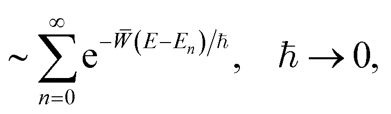
In this paper, an analysis of the instanton rate will be made to show that the first-principles derivation has indeed led to a formula which is asymptotically related to the quantum-mechanical rate. The theory is therefore exact at low temperature in certain limiting cases, which is not true of many other related QTSTs.
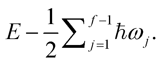
It is well known9,11 that the standard instanton approach fails to predict the rate accurately when the reciprocal temperature β = 1/kBT is near crossover, defined by βc = 2π/ℏ![[small omega, Greek, macron]](https://www.rsc.org/images/entities/i_char_e0da.gif) 0, where 0 is the imaginary frequency at the barrier top. Above the crossover temperature, the instanton orbit does not exist and the theory is not valid.
0, where 0 is the imaginary frequency at the barrier top. Above the crossover temperature, the instanton orbit does not exist and the theory is not valid.
The reason why the instanton rate cannot be used near crossover has been put down to the non-validity of the steepest-descent approximation. Suggestions have been given to correct the results in this regime by including anharmonic terms into the expansion of the Boltzmann operator, e−βĤ.11,47–50 This results in different expressions being used in different temperature regimes and it is not always obvious where one formula should take over from the other.
In this paper, it shall be shown that it is not necessarily the steepest-descent approximations in the position coordinates which are to blame and that the problem can be solved by a different approach. The new approach obtains an approximation to the microcanonical rate over a range of energies, which is weighted by a thermal distribution and integrated numerically to give a single unified formula for semiclassical reaction rates at all temperatures of interest. A number of instantons at different energies will be required in order to do this, although this may not necessarily be a concern for the efficiency of the method. It is often the case that the rate of a reaction is required at multiple temperatures such that a number of independent instanton calculations have to be carried out. Even if the rate at only one temperature is desired, the instanton is often optimized at successively lower temperatures using initial guesses generated from optimizations at higher temperatures. A standard application of instanton theory discards this extra information and only takes one instanton into account. It is not surprising that by retaining all the data, it is possible to formulate a method which gives a higher accuracy.
2 First-principles derivation of instanton theory
In this section, a summary is given of the first-principles derivation of instanton theory from ref. 31 and 38. Although we write the formulae in terms of continuous classical trajectories, the method is intended to be used in the ring-polymer instanton formalism whereby the pathways are discretized as described in ref. 14 and 39.Consider the dynamics of a chemical reaction within the Born–Oppenheimer approximation. The Hamiltonian is Ĥ = |![[p with combining circumflex]](https://www.rsc.org/images/entities/i_char_0070_0302.gif) |2/2m + V(
|2/2m + V(![[x with combining circumflex]](https://www.rsc.org/images/entities/i_char_0078_0302.gif) ), where x = (x0,…,xf−1) are the Cartesian coordinates of f nuclear degrees of freedom. These nuclei move on the potential-energy surface V(x) with conjugate momenta p = (p0,…,pf−1). Without loss of generality, the degrees of freedom have been mass-weighted such that each has the same mass, m.
), where x = (x0,…,xf−1) are the Cartesian coordinates of f nuclear degrees of freedom. These nuclei move on the potential-energy surface V(x) with conjugate momenta p = (p0,…,pf−1). Without loss of generality, the degrees of freedom have been mass-weighted such that each has the same mass, m.
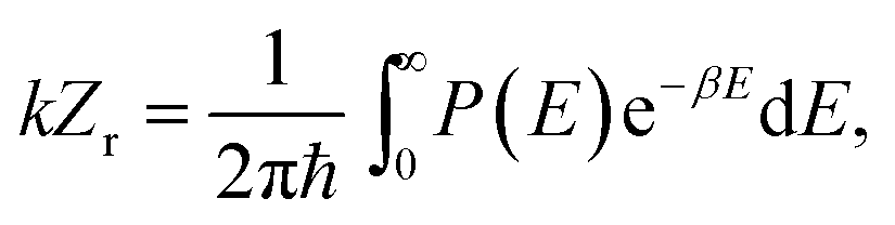
An (f − 1)-dimensional dividing surface, defined by σ(x) = 0, separates reactants, σ < 0, from products, σ > 0. Although it makes no difference to the rate, it is usual to place the dividing surface such that it cuts through the potential barrier. The exact expression for the microcanonical cumulative reaction probability at energy E is51,52
P(E) = 2ℏ2Tr[![[F with combining circumflex]](https://www.rsc.org/images/entities/i_char_0046_0302.gif) ![[thin space (1/6-em)]](https://www.rsc.org/images/entities/char_2009.gif) ImĜ(E)ImĜ(E)], ImĜ(E)ImĜ(E)], | (3) |
 is the flux from reactants to products. The Green's functions will play an important role in this derivation and are defined by
 | (4) |
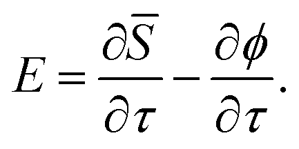
The thermal reaction rate is defined by
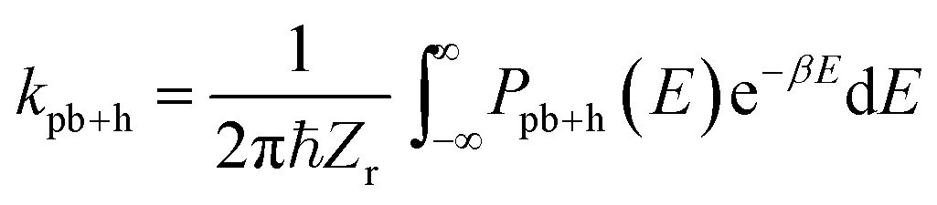
 | (5) |
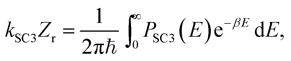
The standard instanton theory was obtained by taking semiclassical approximations to the Green's functions and then evaluating the trace in eqn (3) by steepest-descent integration. A semiclassical approximation to the thermal rate is then obtained by steepest-descent integration of eqn (5). The new approach suggested in this work, however, is to obtain an approximation to P(E) and to integrate over energy numerically.
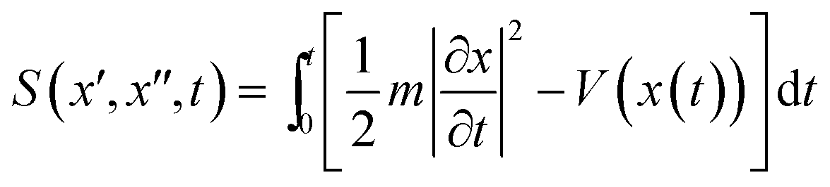
In order to derive a semiclassical approximation to the Green's function, we replace the quantum-mechanical propagator by the van Vleck propagator.53–56 This is the semiclassical limit of Feynman's exact path-integral propagator57 and is defined in terms of a sum over classical trajectories of time t, from x(0) = x′′ to x(t) = x′ to give
 | (6) |
 and the density associated with the trajectory is
 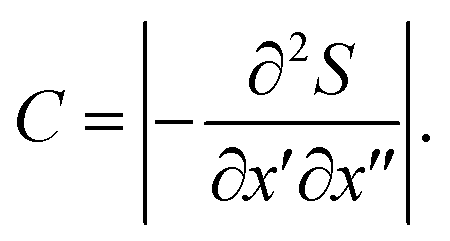 The sign of the square root has to be carefully chosen to keep the function continuous in the complex plane. This gives a phase change of e−iπ/2 when passing through each conjugate point.54–56
The integral over t is then evaluated by the method of steepest descent to give a semiclassical approximation to the Green's function. The stationary points of the exponent solve  and since
  defines the energy of a trajectory passing from x′′ to x′ in time t, they correspond to classical trajectories of energy E.
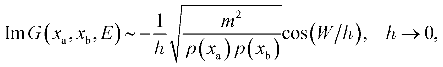
Below the barrier, where E < V(x′′) and E < V(x′), these classical trajectories must evolve in imaginary time such that their kinetic energy is negative. It was found in ref. 38 that trajectories which bounce an odd number of times contribute to the imaginary part of the semiclassical Green's function whereas those which bounce an even number of times (or do not bounce at all) contribute to the real part. A bounce is counted whenever the momentum along the trajectory becomes zero.
As longer imaginary-time trajectories are exponentially damped, the dominant contributions to the imaginary part of the Green's function come from only two trajectories: one which bounces to the left of the dividing surface (t = −iτ−) and the other which bounces to the right (t = −iτ+).
This gives ImG(x′, x′′, E) ∼ Γ− + Γ+ as ħ → 0, where
 | (7) |
 | (8) |
![[S with combining macron]](https://www.rsc.org/images/entities/i_char_0053_0304.gif) ± = −iS(x′, x′′, −iτ±) and
± = −iS(x′, x′′, −iτ±) and 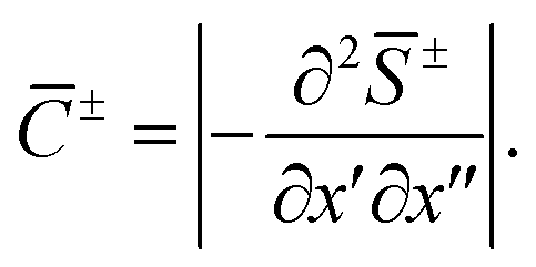 The second line follows from the Legendre transformation
 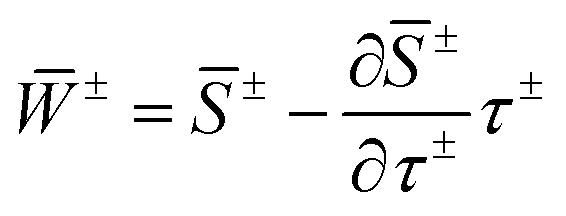 and
and 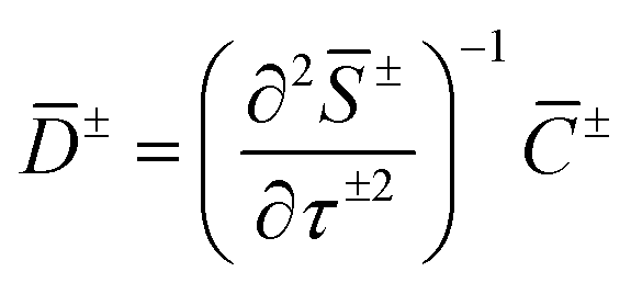 .31,38 The factor of a half appears because the contour of integration only passes through half of the maximum peak in the direction which contributes to the imaginary part of the Green's function. This is explained more fully in Section 4 and ref. 38.
In ref. 31, it was shown that when replacing the Green's functions with their semiclassical approximations,
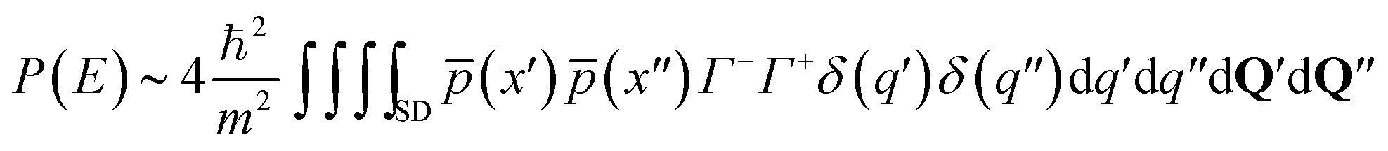 | (9) |
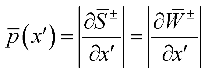 is the magnitude of the momentum of a trajectory at its end point. The coordinate transformation from x to (q, Q) is defined such that q is parallel to the trajectory and equal to 0 at the dividing surface, and Q = (Q1,…,Qf−1) are the perpendicular modes.58 The integrals over the perpendicular modes should also be performed by steepest descent, whereas those over q′ and q′′ can be done exactly due to the presence of the delta functions.
The stationary points are defined by  , where
 ![[W with combining macron]](https://www.rsc.org/images/entities/i_char_0057_0304.gif) = − + +. Here the trajectory which bounces to the left of the dividing surface joins smoothly with that which bounces to the right to form a continuous imaginary-time periodic orbit, called the instanton. Using
= − + +. Here the trajectory which bounces to the left of the dividing surface joins smoothly with that which bounces to the right to form a continuous imaginary-time periodic orbit, called the instanton. Using 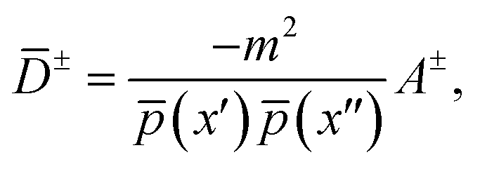 where
where 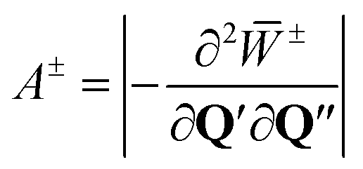 and31,55,56,58
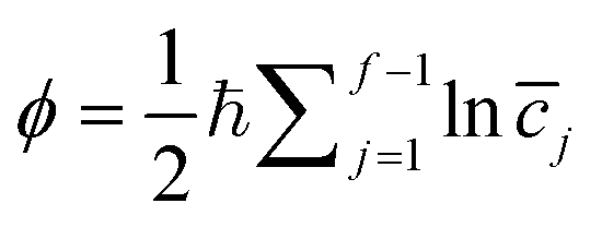
 | (10) |
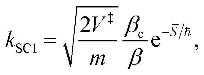
| PSC1(E) = Z‡e−/ℏ. | (11) |
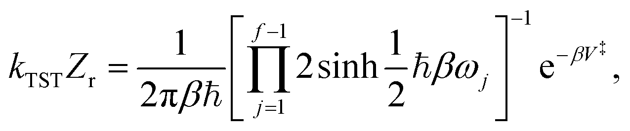
The semiclassical instanton approximation to the thermal rate is obtained from eqn (5) using PSC1(E) and evaluating the integral using the method of steepest descent. In this case the exponent is −/ℏ − βE which can be rearranged to 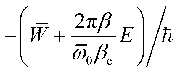 such that it is of the form of eqn (2). We can therefore write k ∼ kSC1 as ħ → 0 for a given value of β/βc, where
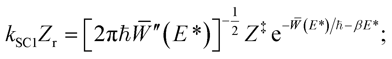 | (12) |
′(E*) = −βℏ, and here primes denote differentiation with respect to E.
In Section 3, we analyse the rates obtained by the instanton approach when applied to an analytically solvable one-dimensional system and suggest a simple way to extend its applicability. The derivation is analysed in Section 4 for a multidimensional problem, and a modification to the steepest-descent approach is suggested which improves the accuracy of the approximation. Section 5 applies the new method to a multidimensional system and compares the results with the standard approach and the exact rates.
3 Analysis of instanton theory applied to a one-dimensional system
In this section, we will analyse the semiclassical instanton approximation to the thermal and microcanonical rate for the one-dimensional symmetric Eckart barrier. The potential is defined by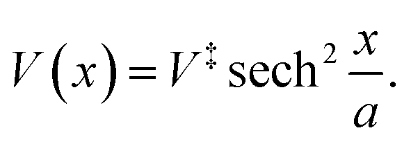 | (13) |
For this surface, the imaginary frequency at the barrier top is 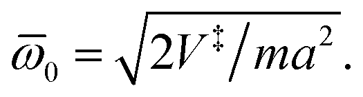 The exact expression for the reaction probability for this system can be given in closed form by59,60
 | (14) |
 and η = E/V‡ is a reduced energy. Throughout this paper, the reaction probability is only defined for energies above the reactant asymptote, E > 0.
When the parameter α is large, the barrier is high and wide and the semiclassical approximations are valid. In fact, asymptotic analysis46 shows that, for a given value of η > 0,
 | (15) |

For this one-dimensional system, the expression for the reaction probability obtained by semiclassical instanton theory, eqn (11), is
 | (16) |
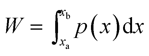
 is the abbreviated action along the instanton pathway and
  are the turning points. For the Eckart barrier it can be evaluated to give the same result as (E) found in eqn (15).60PSC1(E) is of course equal to the well-known WKB approximation for transmission of a one-dimensional barrier.60,61 Note that above the barrier, we have used the semiclassical result as derived in the Appendix. This approximation is formally asymptotically correct for a given value of η obeying 0 < E < V‡ or E > V‡ such that PSC1(E) ∼ P(E) as α → ∞. All these instanton approximations are thus valid for high and wide barriers. However, just because it is asymptotically related to the exact result does not mean that it is a good approximation for finite α. For instance, it is obviously a poor approximation at energies near the barrier when (E) becomes small. Formally, this is because there is no such asymptotic relation at E = V‡, at which point PSC1(V‡) = 1, whereas
There is a simple way to correct this error in the SC1 expression, by replacing it with the asymptotic result of eqn (15). For more general potential-energy surfaces, the value of (E) is not known analytically but can be obtained numerically by an instanton calculation. However, this will only be possible when (E) is available, i.e. for energies lower than the barrier height when the instanton exists.
Near the barrier top or above it, the instanton is collapsed so knowledge is only required for a small region about the transition state. As it is assumed that all potential-energy barriers have the parabolic form,  in this small region around their top, we can use the corresponding transmission to improve the semiclassical result. The exact result for this case is Ppb(E) = [1 + epb(E)/ℏ]−1, where pb(E) = 2π(V‡ − E)/0 is the abbreviated action for the parabolic barrier.60
We can therefore suggest the form of an improved instanton theory, which we call the SC3 approximation,
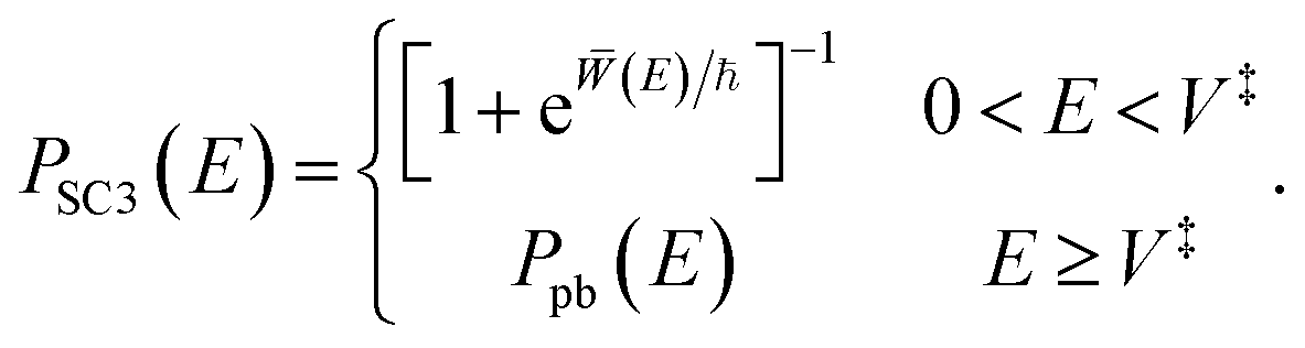 | (17) |
Asymptotic approximations are not unique and adding higher-order terms is always possible. A simple justification of eqn (17) is that it doesn't break any of the asymptotic relations which existed previously, and now in fact PSC3(E) ∼ P(E) as α → ∞ for all E > 0. Eqn (17) was previously suggested by Kemble60,62,63 based on a WKB analysis. To calculate PSC3(E), we require no more information than is obtained in a typical instanton calculation, i.e. the abbreviated action (E) and the imaginary barrier frequency 0.
Note that eqn (17) is exact for a parabolic barrier. Because the exact transmission for the Eckart barrier is asymptotic to the parabolic barrier for E ≥ V‡, PSC3(E) is an asymptotic limit for the Eckart barrier at all energies. One therefore assumes that it will also be a good approximation for real chemical systems, which tend to have potential barriers of a similar shape.
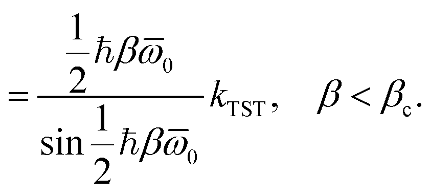
The SC1 approximation to the thermal rate is defined by eqn (12), where for this one-dimensional system Z‡ = 1 and  is the translational partition function of the reactants per unit length. For the Eckart barrier, whose crossover temperature is given by βc = α/V‡, this can be expressed analytically using the location of the stationary point, E*/V‡ = βc2/β2, which gives
 | (18) |
= ℏα(2 − βc/β).
This result is exact in the limit that α → ∞ for a given value of β/βc. Such an asymptotic relation does not exist for many other approximate quantum rate theories. For instance, h-RPTST is defined by performing the integrals in RPTST by steepest descent;14 this gives a rate with the correct exponent but a slightly different prefactor from that obtained by SC1.‡ This suggests that instanton rate theory gives the more fundamental description of deep tunnelling and shows that the quantum transition-state theory approximation which leads to RPTST64,65 is not exact, even in the limiting case of a high and wide barrier. This explains the observation that the free-energy version of instanton theory is superior to RPTST at low temperatures for the atom–diatom scattering calculations performed in ref. 66.
Of course RPTST performs well at higher temperatures where it tends to classical transition-state theory. Unlike RPTST, the SC1 rate suffers from problems near the crossover temperature due partly to the errors in eqn (16) and partly to the steepest-descent approximation for the energy integral. An improved thermal rate can be defined using eqn (17) as
 | (19) |
Using the two different approximations described so far we obtain the thermal rate constants shown in Fig. 1 for a model system describing a proton transfer.
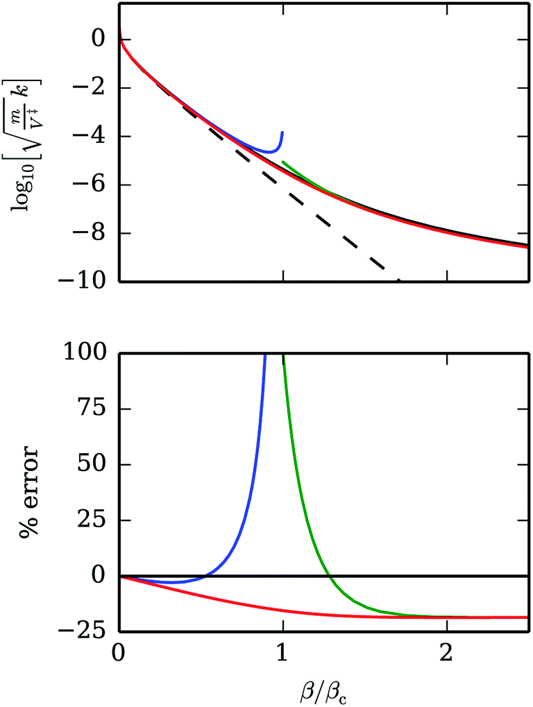 | ||
| Fig. 1 In the upper panel, dimensionless thermal rates calculated for the Eckart barrier are shown with various levels of theory: exact (black), classical (dashed), parabolic barrier (blue), standard semiclassical instanton SC1 (green), new improved instanton SC3 (red). In this example, the parameter α = 12 is chosen to replicate results from ref. 14 and 34. Relative errors are given in the lower panel per cent. | ||
Of course, none of the semiclassical results is exact because the value of α is given by the chemical barrier under study and cannot be made arbitrarily large. The SC3 rates coincide with the SC1 approximation at low temperatures because in this region the instantons are much lower than the barrier height, making PSC1(E) ≈ PSC3(E), and the steepest-descent integration over energy is accurate. At high temperatures, kSC3 correctly tends to the classical result, which is a consequence of the quantum-classical correspondence principle. The major improvement of the SC3 instanton approximation over the standard approaches is that the rates are also accurate in the region of the crossover temperature. It avoids the discontinuity and remains finite at all temperatures. For this value of α, the error remains below 25%, which is often quite acceptable in a chemical reaction rate calculation and probably cannot be beaten by other approximate path-integral rate theories.
Before a general version of the improved SC3 approximation can be obtained, we must look more closely at the microcanonical approximations for the case of a multidimensional system.
4 Microcanonical instanton theory
It was already noted by Chapman et al.2 that there is a problem with the semiclassical instanton estimation of microcanonical rates in multidimensional systems. This becomes apparent by considering a separable two-dimensional system of a barrier uncoupled to a harmonic well with frequency ω1 and eigenstates The correct cumulative reaction probability for this reaction is related to the transmission of the one-dimensional barrier, P1D(E) by
 | (20) |
 | (21) |
 | (22) |
(E) is the abbreviated action of the instanton orbit, u1(E) = ω1τ is the stability parameter, 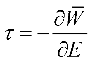 is the imaginary period, and we have used a series expansion for the hyperbolic function. Eqn (22) is only a good approximation to eqn (21) in the limit that u(E) → 0.§ However, in molecular systems, it is quite common for the vibrational frequencies to be large and for this approximation to fail. Worse, it is defined only for E < V‡ and a significant zero-point energy contribution from the vibrational modes will make the method unable to study the transmission anywhere near the barrier top, which occurs at V‡ + E0.
An improved result is obtained by taking a slightly different steepest-descent approximation in the derivation of the Green's function from that of Section 2. Taking as an example a parabolic barrier uncoupled to a set of f − 1 harmonic oscillators, 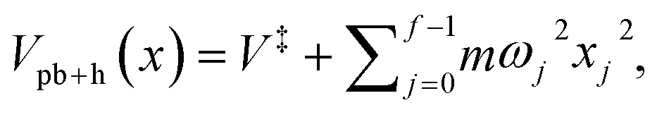 where ω0 = i0 and 0 > 0, whereas ωj > 0 for j > 0. The classical action is given by
 | (23) |
 | (24) |
In the approach followed in Section 2, we would now perform a steepest-descent approximation to the integral in eqn (6) to obtain a semiclassical approximation to Ĝ. The conjugate times, given by t = nπ/ωj for n ∈ ![[Doublestruck Z]](https://www.rsc.org/images/entities/char_e17d.gif) , are poles of the integrand. For E < V(x′) and E < V(x′′), the exponent, iS/ħ + iEt/ħ, has a series of stationary points at imaginary times corresponding to all possible direct or bouncing trajectories under the parabolic barrier. We deform the contour of integration to the one shown in Fig. 2, which is a path of steepest descent of the exponent and passes through its stationary points. By Jordan's lemma, the integral along this contour is equal to the one in eqn (6) since we can give E an infinitesimal positive imaginary part to ensure that the integrand tends to 0 as t → ∞. As shown above, this approach gives poor results for the microcanonical cumulative reaction probability of multidimensional systems. However, when the low-temperature thermal reaction rate is obtained by steepest-descent evaluation of eqn (5), it apparently gives good results again. This is probably due to an error cancellation, which is as yet unidentified.
, are poles of the integrand. For E < V(x′) and E < V(x′′), the exponent, iS/ħ + iEt/ħ, has a series of stationary points at imaginary times corresponding to all possible direct or bouncing trajectories under the parabolic barrier. We deform the contour of integration to the one shown in Fig. 2, which is a path of steepest descent of the exponent and passes through its stationary points. By Jordan's lemma, the integral along this contour is equal to the one in eqn (6) since we can give E an infinitesimal positive imaginary part to ensure that the integrand tends to 0 as t → ∞. As shown above, this approach gives poor results for the microcanonical cumulative reaction probability of multidimensional systems. However, when the low-temperature thermal reaction rate is obtained by steepest-descent evaluation of eqn (5), it apparently gives good results again. This is probably due to an error cancellation, which is as yet unidentified.
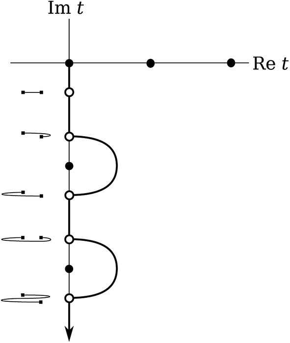 | ||
| Fig. 2 Argand diagram for the separable parabolic + harmonic system. Filled circles represent poles of the integrand and open circles represent stationary points of the exponent. Assuming x′0 + x′′0 > 0, they correspond to the trajectories depicted in position space to the side of each stationary point. The second and third stationary points, located at −iτ+ and −iτ−, are those which contribute to the imaginary part of the semiclassical Green's function. As they are saddle points, i.e. maxima in one direction and minima in the other, they only contribute as the steepest-descent contour departs (and not as it arrives), thus giving a factor of half to the integral. | ||
The reason for the poor result is, however, now clear. Making the variable transformation t = −iτ gives  and
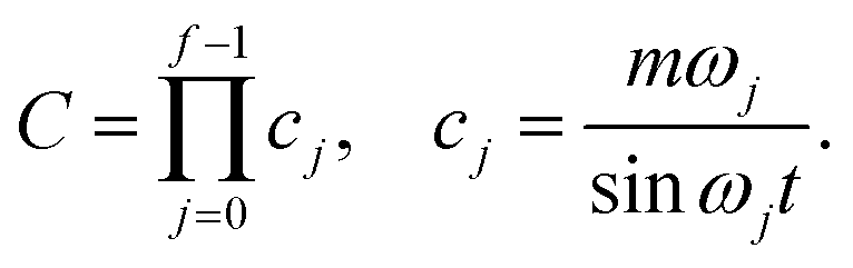
and ![[c with combining macron]](https://www.rsc.org/images/entities/i_char_0063_0304.gif) j = −icj = mωj/sinhωjτ. On the negative imaginary-t axis, it becomes apparent that j (j ≥ 1) acquires an exponential dependence on τ and should thus be treated as part of the exponential rather than the prefactor in the steepest-descent approximation. This is especially important when ωj is large, which is commonly the case in chemical applications. This is not true of 0 = m0/sin0τ which remains oscillatory. We therefore rewrite eqn (6) as
j = −icj = mωj/sinhωjτ. On the negative imaginary-t axis, it becomes apparent that j (j ≥ 1) acquires an exponential dependence on τ and should thus be treated as part of the exponential rather than the prefactor in the steepest-descent approximation. This is especially important when ωj is large, which is commonly the case in chemical applications. This is not true of 0 = m0/sin0τ which remains oscillatory. We therefore rewrite eqn (6) as
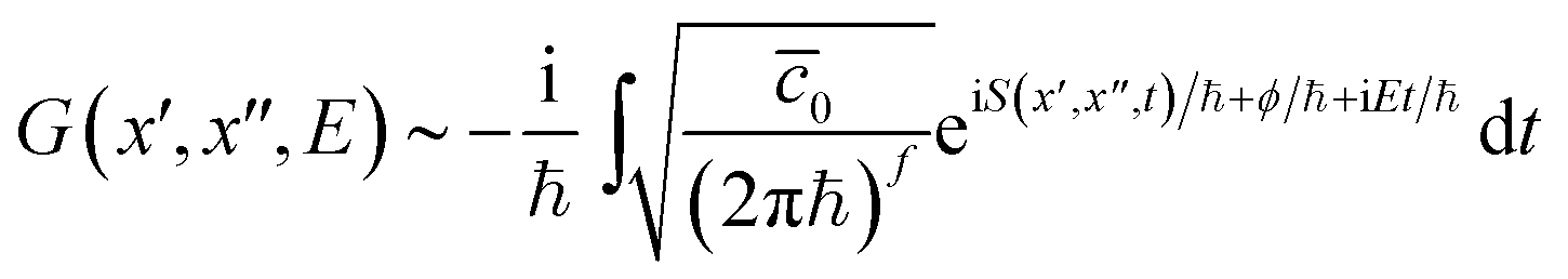 | (25) |
 and the integration contour is depicted in Fig. 2.
Stationary points of the exponent are defined by values of t which solve
 | (26) |
 | (27) |
Although the addition of ϕ shifts the stationary points slightly, for low enough E, they remain on the imaginary axis such that the schematic in Fig. 2 still represents the steepest-descent integration contour. Note that for the case of harmonic oscillators with high frequency,
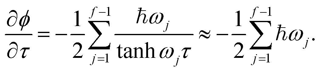 | (28) |
The total energy is therefore the sum of the instanton energy,  and the zero-point energy of perpendicular modes,
Because of the phase change after the conjugate time t = −iπ/0 and taking into account the direction of the steepest-descent contour, it is the single-bounce trajectories which contribute to the leading asymptotic terms for the imaginary part of the Green's function. Their imaginary times, which solve eqn (27), are denoted τ± depending on whether it bounces once on the right or left of the dividing surface. The three other trajectories depicted in Fig. 2 only contribute to ReĜ and not therefore to the rate. As before, the total imaginary part of the Green’s function is ImG(x′, x′′, E) ∼ Γ+ + Γ− as ħ → 0, where Γ± is the contribution from just one of these trajectories but is now defined by
 | (29) |
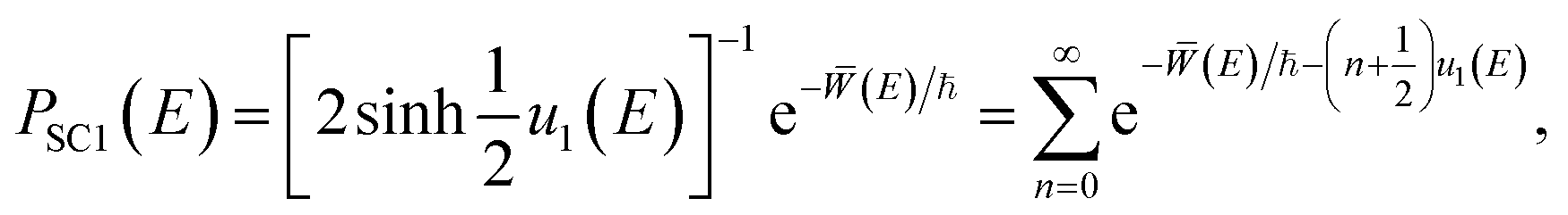
Applying the new definition of Γ± to eqn (9), we obtain the SC2 approximation for the microcanonical cumulative reaction probability,
 | (30) |
Note that the SC1 and SC2 approximations are equivalent for a one-dimensional system but that the SC2 result is expected to perform better in multidimensional problems. For the case that we have a separable system of a one-dimensional barrier uncoupled to a set of harmonic oscillators of high frequency, such that  , the results reduce to
 | (31) |
 | (32) |
 In the limit of high frequencies, this gives
| PSC2(E) = e−/ℏ, | (33) |
 This is the leading term of eqn (21), equivalent to assuming that the perpendicular modes are all in their ground states. We have thus managed to obtain an instanton approximation to a microcanonical rate which is a good approximation both for one-dimensional and multidimensional systems, and is applicable for energies at least up to the barrier height plus the zero-point energy of the perpendicular modes.
We apply the barrier-top correction of Section 3 also to the multidimensional microcanonical cumulative reaction probability to give
 | (34) |
 is defined as the highest energy for which the corresponding instanton remains stretched. Once it is collapsed, we switch to the exact result for the parabolic + harmonic system,
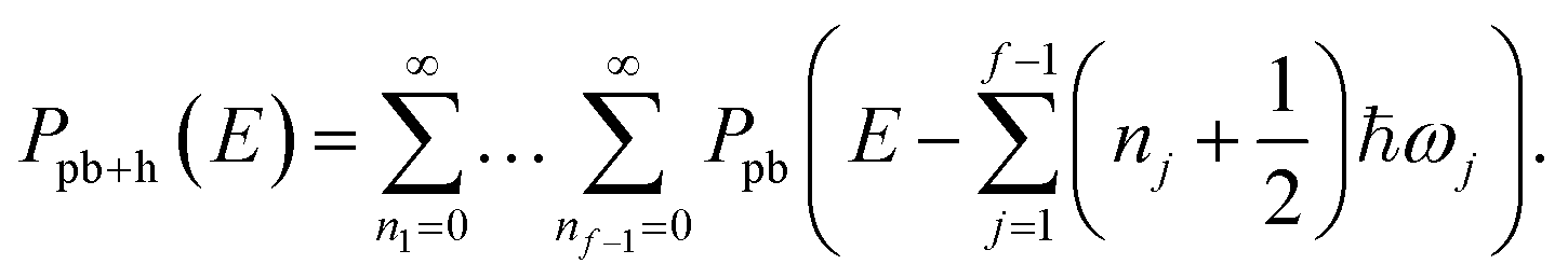 | (35) |
Unfortunately, this does not necessarily match exactly with the microcanonical instanton approximation just below the barrier. This is not a significant problem as the integral in eqn (5) will smooth out the discontinuity and give a continuous function of k with respect to β.
In practice, rather than solving the transcendental equation eqn (27) for τ± for a given value of E, one can use it to define E directly from a given value of τ. Trajectories can then be optimized using the usual ring-polymer instanton approach.14,39 A number of values of τ will be required in order to evaluate the integral, and each will require an independent calculation of an instanton. Derivatives of ϕ± with respect to τ± can be obtained by finite differences by reoptimizing trajectories with slightly longer and slightly shorter imaginary times, keeping the end-points fixed.
Although these formulae were derived with the parabolic + harmonic system in mind, the approach is also valid for more general systems. There are however a number of ways in which ϕ could be defined for a nonseparable system. In anharmonic and asymmetric systems, it may happen that 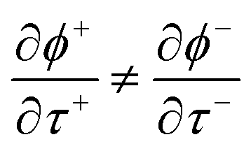 such that there is not a unique definition for the total energy represented by the instanton. In these cases, it may be possible to simply average the two results. Tests will have to be performed to discover which precise definition performs best over a wide range of problems.
5 Thermal instanton rate theory
As in the one-dimensional case, the thermal reaction rate of a multidimensional system is obtained from the cumulative reaction probability using numerical integration of eqn (19). After computing PSC3(E) at a range of energies, the thermal rate can be obtained at many different temperatures without recomputing any instantons. To be consistent with the semiclassical approximations, the appropriate reactant partition function per unit volume should be used, employing harmonic approximations for the vibrational modes.Here, we compare the results of various approaches on a simple test system with parameters chosen to model the transition state of the gas-phase H + H2 reaction. A two-dimensional potential is defined as an uncoupled sum of the Eckart barrier, eqn (13), with V‡ = 0.425 eV and a = 0.734 a.u., in one direction and a harmonic oscillator, with ω1 = 2055 cm−1, in the other. The mass was chosen to be m = 1061 a.u. This system has a crossover temperature given by βc ≈ 850 a.u. and a zero-point energy of 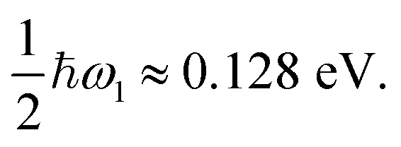 The reactant partition function per unit length is
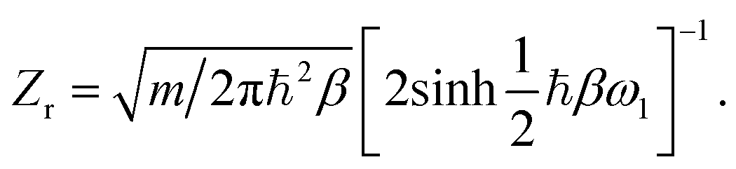
For comparison, the rate given by Eyring's TST,67 which neglects tunnelling effects, is given by
 | (36) |
 | (37) |
 | (38) |
Results for the microcanonical rate are presented in Table 1 and for thermal rates in Table 2. The results of the SC3 approximation compare very well with the exact rates throughout and the relative errors remain below 20%, whereas each of the other approximations fails in particular regimes. At higher energies than those presented in Table 1, the SC2/SC3 instanton becomes collapsed and the parabolic barrier expression is used. This is a good approximation in this regime.
| E/eV | P pb+h(E) | P SC1(E) | P SC3(E) | P(E) |
|---|---|---|---|---|
| 0.15 | 3.48(−6) | 2.57(−8) | 1.35(−9) | 1.61(−9) |
| 0.20 | 1.66(−5) | 7.25(−7) | 1.72(−7) | 2.07(−7) |
| 0.25 | 7.91(−5) | 1.15(−5) | 4.60(−6) | 5.54(−6) |
| 0.30 | 3.77(−4) | 1.26(−4) | 6.57(−5) | 7.92(−5) |
| 0.35 | 1.79(−3) | 1.07(−3) | 6.52(−4) | 7.85(−4) |
| 0.40 | 8.50(−3) | 7.49(−3) | 5.03(−3) | 6.06(−3) |
| 0.45 | 3.92(−2) | — | 3.17(−2) | 3.80(−2) |
| 0.50 | 1.63(−1) | — | 1.56(−1) | 1.82(−1) |
| 0.55 | 4.82(−1) | — | 4.81(−1) | 5.28(−1) |
| β | k TST | k pb+h or kSC1 | k SC3 | k |
|---|---|---|---|---|
| 100 | 2.6(−4) | 2.6(−4) | 2.6(−4) | 2.7(−4) |
| 250 | 1.6(−5) | 1.8(−5) | 1.8(−5) | 1.9(−5) |
| 500 | 2.2(−7) | 4.3(−7) | 3.8(−7) | 4.2(−7) |
| 840 | 8.5(−10) | 7.1(−8) | 4.5(−9) | 5.2(−9) |
| 860 | 6.1(−10) | 7.9(−9) | 3.5(−9) | 4.1(−9) |
| 1000 | 6.4(−11) | 1.1(−9) | 7.8(−10) | 9.3(−10) |
| 1500 | 2.1(−14) | 1.7(−11) | 1.7(−11) | 2.0(−11) |
| 2000 | 7.4(−18) | 1.9(−12) | 1.9(−12) | 2.3(−12) |
k TST is of course unable to describe tunnelling and is many orders of magnitude too small at low temperatures. The parabolic barrier approximation to the microcanonical rate becomes good near the barrier top. The thermal rate based on this approximation is good at high temperatures but in error near and below the crossover temperature, where it tends to infinity and becomes undefined. The standard SC1 instanton rates are equal to the SC3 approximation at low temperature but perform poorly near crossover. PSC1(E) cannot be obtained for E > V‡ and is obviously inferior to the SC3 approximation at low energies.
6 Discussion
We have shown that instanton theory is a powerful technique for studying chemical reactions and is one of the few approximate methods which gives the exact rate in the limiting case of a high and wide barrier. Knowledge of the new first-principles derivation has been used to extend the method beyond its former capabilities and define an accurate microcanonical rate theory which can be numerically integrated to give a thermal rate at any temperature. This avoids the discontinuity problem at the crossover temperature without significantly changing the computational algorithms required for implementation of the instanton approach.A nice consequence of the new SC3 approach is that the data obtained by each instanton calculation is used to compute the thermal rate. In contrast, the standard SC1 approach throws away the information from all but one instanton.
The microcanonical instanton formulation opens the possibility of studying reactions initiated from certain non-equilibrium conditions. It could also be weighted by more general distributions than the Boltzmann distribution to give non-thermal rates.
Some of the new formulae given in this paper are similar, although not equivalent, to expressions suggested in previous work. In particular Chapman, Garret and Miller2 recognized the problems with PSC1(E) in multidimensional systems and corrected it by replacing terms of the form eqn (22) with eqn (21). It is good to see that a similar transformation can be achieved more rigorously using an extension of the usual steepest-descent integration. Kryvohuz27 has also suggested an instanton method which can avoid the problems of the thermal rate near the crossover temperature. This was done by truncating the steepest-descent integral over energy at the barrier top to give an error function. Above the crossover temperature, an alternative formula was used. This was first derived by Cao and Voth47 from a fourth-order expansion of the potential about the barrier top.
Of course, instanton theory cannot be applied directly to chemical reactions in solution, as in these systems, too many imaginary-time classical trajectories contribute. For such studies, path-integral methods such as RPMD37 are obviously more appropriate. However, it is only through the underlying instanton theory that we fully understand how the RPMD approach works14 and will be able to find ways of extending it to new problems.
The first-principles derivation of instanton theory makes it clear that only the imaginary-time trajectories which bounce are able to contribute to the imaginary part of the Green's function and hence to the rate. It is the fact that we need to only sample bouncing trajectories which makes accurate path-integral transition-state theories difficult to define. The optimum dividing surface chosen by RPTST is devised to bias towards ring-polymer configurations which are stretched and thus contribute to ImĜ. The quantum instanton approach68,69 utilizes two dividing surfaces for the same reason—because it is necessary to ensure that the sampled configurations are stretched. This was not necessary for the semiclassical instanton, where it is easier to categorize trajectories as direct or bouncing and thus to keep only the relevant parts. If we are to develop new path-integral rate theories based on sampling ring polymers, it will be necessary to find a way of sampling only the correct configurations which contribute to ImĜ. Work is in progress in this area.
7 Appendix: semiclassical rate above the barrier
To show the universality of the semiclassical Green's function approach, the rate over the barrier will be derived in this way. For simplicity, we take a one-dimensional system and choose two dividing surfaces σa(x) = x − xa and σb(x) = x − xb with xa < xb. The exact microcanonical cumulative reaction probability can be defined by52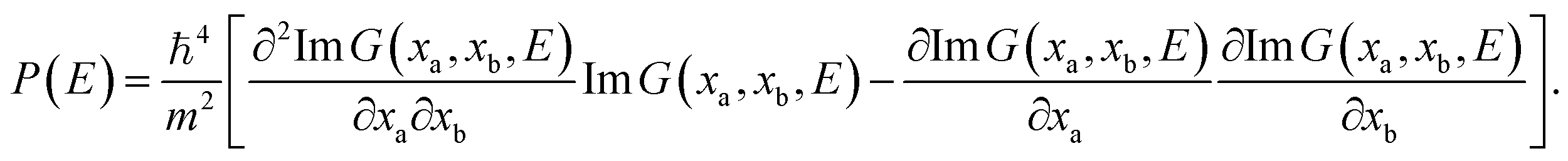 | (39) |
Assuming that E is larger than the barrier height, the semiclassical approximation to the Green's functions is found using the direct real-time trajectory between xa and xb;38
 | (40) |
 and
and 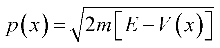 .
.
Therefore the semiclassical approximation to the cumulative reaction probability above the barrier is
 | (41) |
Wigner's quantum correction to the thermal rate70 is written as a series in powers of ħ, where the first term is the classical rate. The semiclassical method includes no tunnelling corrections above the barrier because it only returns the leading-order term. Only below the barrier, where the classical rate is zero, does the leading-order term include tunnelling. In eqn (17), the SC3 result is improved using the exact result for the parabolic barrier which includes all terms.
A full semiclassical study of the multidimensional problem above the barrier would involve a search for real-time periodic trajectories in a similar way to Gutzwiller's trace formalism.55 These can travel perpendicular to the reaction coordinate and be very long, complicated and chaotic, making the method more involved than a standard instanton calculation. We therefore content ourselves with using the exact result for the parabolic barrier with perpendicular harmonic modes in all cases. By doing this, we have effectively made a harmonic approximation to the perpendicular coordinates. This separable approximation is not appropriate below the barrier, where the instanton provides a better description,71 but leads to the Eyring TST formula67 at high temperatures, which is often an acceptable approximation in these limits.
Acknowledgements
This work was supported by a European Union COFUND/Durham Junior Research Fellowship.References
- W. H. Miller, J. Chem. Phys., 1975, 62, 1899–1906 CrossRef CAS.
- S. Chapman, B. C. Garrett and W. H. Miller, J. Chem. Phys., 1975, 63, 2710–2716 CrossRef CAS.
- J. S. Langer, Ann. Phys., 1967, 41, 108–157 CAS.
- J. S. Langer, Ann. Phys., 1969, 54, 258–275 CAS.
- M. Stone, Phys. Lett. B, 1977, 67, 186–188 CrossRef.
- S. Coleman, Phys. Rev. D: Part. Fields, 1977, 15, 2929 CrossRef.
- C. G. Callan Jr and S. Coleman, Phys. Rev. D: Part. Fields, 1977, 16, 1762 CrossRef.
- S. Coleman, Proc. Int. School of Subnuclear Physics, 1977 Search PubMed.
- I. Affleck, Phys. Rev. Lett., 1981, 46, 388–391 CrossRef.
- A. O. Caldeira and A. J. Leggett, Ann. Phys., 1983, 149, 374–456 Search PubMed.
- U. Weiss, Quantum Dissipative Systems, World Scientific, Singapore, 4th edn, 2012 Search PubMed.
- V. A. Benderskii, D. E. Makarov and C. A. Wight, Chemical Dynamics at Low Temperatures, Wiley, New York, 1994, vol. 88 Search PubMed.
- W. Siebrand, Z. Smedarchina, M. Z. Zgierski and A. Fernández-Ramos, Int. Rev. Phys. Chem., 1999, 18, 224105 CrossRef.
- J. O. Richardson and S. C. Althorpe, J. Chem. Phys., 2009, 131, 214106 CrossRef PubMed.
- S. Andersson, G. Nyman, A. Arnaldsson, U. Manthe and H. Jónsson, J. Phys. Chem. A, 2009, 113, 4468–4478 CrossRef CAS PubMed.
- S. Andersson, T. P. M. Goumans and A. Arnaldsson, Chem. Phys. Lett., 2011, 513, 31 CrossRef CAS.
- H. Jónsson, Proc. Natl. Acad. Sci. U. S. A., 2011, 108, 944–949 CrossRef PubMed.
- R. Pérez de Tudela, Y. V. Suleimanov, J. O. Richardson, V. Sáez Rábanos, W. H. Green and F. J. Aoiz, J. Phys. Chem. Lett., 2014, 5, 4219–4224 CrossRef PubMed.
- T. P. M. Goumans and J. Kästner, Angew. Chem., Int. Ed., 2010, 49, 7350–7352 CrossRef CAS PubMed.
- T. P. M. Goumans and J. Kästner, J. Phys. Chem. A, 2011, 115, 10767 CrossRef CAS PubMed.
- J. Meisner, J. B. Rommel and J. Kästner, J. Comput. Chem., 2011, 32, 3456 CrossRef CAS PubMed.
- J. B. Rommel, T. P. M. Goumans and J. Kästner, J. Chem. Theory Comput., 2011, 7, 690–698 CrossRef CAS PubMed.
- J. B. Rommel and J. Kästner, J. Chem. Phys., 2011, 134, 184107 CrossRef PubMed.
- J. B. Rommel, Y. Liu, H.-J. Werner and J. Kästner, J. Phys. Chem. B, 2012, 116, 13682–13689 CrossRef CAS PubMed.
- J. Kästner, Chem.–Eur. J., 2013, 19, 8207–8212 CrossRef PubMed.
- J. Kästner, WIREs Comput. Mol. Sci., 2014, 4, 158–168 CrossRef.
- M. Kryvohuz, J. Chem. Phys., 2011, 134, 114103 CrossRef PubMed.
- M. Kryvohuz and R. Marcus, J. Chem. Phys., 2012, 137, 134107 CrossRef CAS PubMed.
- M. Kryvohuz, J. Chem. Phys., 2012, 137, 234304 CrossRef PubMed.
- M. Kryvohuz, J. Phys. Chem. A, 2014, 118, 535–544 CrossRef CAS PubMed.
- J. O. Richardson, J. Chem. Phys., 2016, 144, 114106 CrossRef PubMed.
- S. C. Althorpe, J. Chem. Phys., 2011, 134, 114104 CrossRef PubMed.
- M. J. Gillan, J. Phys. C: Solid State Phys., 1987, 20, 3621–3641 CrossRef.
- G. A. Voth, D. Chandler and W. H. Miller, J. Chem. Phys., 1989, 91, 7749 CrossRef CAS.
- G. A. Voth, D. Chandler and W. H. Miller, J. Phys. Chem., 1989, 93, 7009–7015 CrossRef CAS.
- I. R. Craig and D. E. Manolopoulos, J. Chem. Phys., 2005, 123, 034102 CrossRef PubMed.
- S. Habershon, D. E. Manolopoulos, T. E. Markland and T. F. Miller III, Annu. Rev. Phys. Chem., 2013, 64, 387–413 CrossRef CAS PubMed.
- J. O. Richardson, R. Bauer and M. Thoss, J. Chem. Phys., 2015, 143, 134115 CrossRef PubMed.
- J. O. Richardson, J. Chem. Phys., 2015, 143, 134116 CrossRef PubMed.
- P. G. Wolynes, J. Chem. Phys., 1987, 87, 6559 CrossRef.
- J. Cao, C. Minichino and G. A. Voth, J. Chem. Phys., 1995, 103, 1391 CrossRef CAS.
- J. Cao and G. A. Voth, J. Chem. Phys., 1997, 106, 1769 CrossRef CAS.
- J. Cao and G. A. Voth, J. Chem. Phys., 1998, 109, 2043 CrossRef CAS.
- C. D. Schwieters and G. A. Voth, J. Chem. Phys., 1998, 108, 1055 CrossRef CAS.
- C. D. Schwieters and G. A. Voth, J. Chem. Phys., 1999, 111, 2869 CrossRef CAS.
- C. M. Bender and S. A. Orszag, Advanced Mathematical Methods for Scientists and Engineers, McGraw-Hill, New York, 1978 Search PubMed.
- J. Cao and G. A. Voth, J. Chem. Phys., 1996, 105, 6856–6870 CrossRef CAS.
- Y. Zhang, J. B. Rommel, M. T. Cvitaš and S. C. Althorpe, Phys. Chem. Chem. Phys., 2014, 16, 24292–24300 RSC.
- M. Kryvohuz, J. Chem. Phys., 2013, 138, 244114 CrossRef PubMed.
- G. Mills, G. K. Schenter, D. E. Makarov and H. Jónsson, Chem. Phys. Lett., 1997, 278, 91 CrossRef CAS.
- W. H. Miller, J. Chem. Phys., 1974, 61, 1823 CrossRef CAS.
- W. H. Miller, S. D. Schwartz and J. W. Tromp, J. Chem. Phys., 1983, 79, 4889 CrossRef CAS.
- J. H. van Vleck, Proc. Natl. Acad. Sci. U. S. A., 1928, 14, 178 CrossRef CAS.
- M. C. Gutzwiller, J. Math. Phys., 1967, 8, 1979 CrossRef CAS.
- M. C. Gutzwiller, Chaos in Classical and Quantum Mechanics, Springer-Verlag, New York, 1990 Search PubMed.
- H. Kleinert, Path Integrals in Quantum Mechanics, Statistics, Polymer Physics and Financial Markets, World Scientific, Singapore, 5th edn, 2009 Search PubMed.
- R. P. Feynman and A. R. Hibbs, Quantum Mechanics and Path Integrals, McGraw-Hill, New York, 1965 Search PubMed.
- M. C. Gutzwiller, J. Math. Phys., 1971, 12, 343 CrossRef.
- C. Eckart, Phys. Rev., 1930, 35, 1303 CrossRef CAS.
- R. P. Bell, The Tunnel Effect in Chemistry, Chapman and Hall, London, 1980 Search PubMed.
- R. P. Bell, Proc. R. Soc. London, Ser. A, 1935, 148, 241–250 CrossRef CAS.
- E. C. Kemble, Phys. Rev., 1935, 48, 549 CrossRef.
- E. C. Kemble, The Fundamental Principles of Quantum Mechanics, McGraw-Hill, 1937 Search PubMed.
- T. J. H. Hele and S. C. Althorpe, J. Chem. Phys., 2013, 138, 084108 CrossRef PubMed.
- S. C. Althorpe and T. J. H. Hele, J. Chem. Phys., 2013, 139, 084115 CrossRef PubMed.
- Y. Zhang, T. Stecher, M. T. Cvitaš and S. C. Althorpe, J. Phys. Chem. Lett., 2014, 5, 3976–3980 CrossRef CAS PubMed.
- H. Eyring, Trans. Faraday Soc., 1938, 34, 41–48 RSC.
- W. H. Miller, Y. Zhao, M. Ceotto and S. Yang, J. Chem. Phys., 2003, 119, 1329 CrossRef CAS.
- J. Vaníček, W. H. Miller, J. F. Castillo and F. J. Aoiz, J. Chem. Phys., 2005, 123, 054108 CrossRef PubMed.
- E. Wigner, J. Phys. Chem. B, 1932, 19, 203–216 Search PubMed.
- W. H. Miller, Acc. Chem. Res., 1993, 26, 174 CrossRef CAS.
Footnotes |
| † See ref. 46 for the derivation and a fuller discussion of the validity of this relation. |
| ‡ The extra prefactor term was called αh(β) in ref. 14. |
| § It also happens to be exact for the special case of a parabolic barrier. |
| This journal is © The Royal Society of Chemistry 2016 |