High-throughput quantum cascade laser (QCL) spectral histopathology: a practical approach towards clinical translation

Abstract

Infrared microscopy has become one of the key techniques in the biomedical research field for interrogating tissue. In partnership with multivariate analysis and machine learning techniques, it has become widely accepted as a method that can distinguish between normal and cancerous tissue with both high sensitivity and high specificity. While spectral histopathology (SHP) is highly promising for improved clinical diagnosis, several practical barriers currently exist, which need to be addressed before successful implementation in the clinic. Sample throughput and speed of acquisition are key barriers and have been driven by the high volume of samples awaiting histopathological examination. FTIR chemical imaging utilising FPA technology is currently state-of-the-art for infrared chemical imaging, and recent advances in its technology have dramatically reduced acquisition times. Despite this, infrared microscopy measurements on a tissue microarray (TMA), often encompassing several million spectra, takes several hours to acquire. The problem lies with the vast quantities of data that FTIR collects; each pixel in a chemical image is derived from a full infrared spectrum, itself composed of thousands of individual data points. Furthermore, data management is quickly becoming a barrier to clinical translation and poses the question of how to store these incessantly growing data sets. Recently, doubts have been raised as to whether the full spectral range is actually required for accurate disease diagnosis using SHP. These studies suggest that once spectral biomarkers have been predetermined it may be possible to diagnose disease based on a limited number of discrete spectral features. In this current study, we explore the possibility of utilising discrete frequency chemical imaging for acquiring high-throughput, high-resolution chemical images. Utilising a quantum cascade laser imaging microscope with discrete frequency collection at key diagnostic wavelengths, we demonstrate that we can diagnose prostate cancer with high sensitivity and specificity. Finally we extend the study to a large patient dataset utilising tissue microarrays, and show that high sensitivity and specificity can be achieved using high-throughput, rapid data collection, thereby paving the way for practical implementation in the clinic.

---

1 Introduction

Histopathology is currently the gold standard for identifying the manifestation of disease in tissue. Principally relying on changes in morphology and architecture highlighted through selective staining,^1,2 a highly trained pathologist can diagnose disease, suggest possible treatments and even provide information on likely prognosis. Microscopic examination of stained tissue biopsy sections presents the pathologist with a high degree of information, and histopathology is currently unsurpassed in its diagnostic accuracy. However, manual examination of individual tissue biopsies is extremely time-consuming, with each section being individually interrogated for the presence of abnormalities. Limited throughput inevitably results in significant delays between the time a biopsy is obtained and a diagnosis being made, with clear implications for patient care and treatment. Furthermore disease diagnosis based on tissue morphology and architecture is inherently subjective, often resulting in intra- and inter-observer error.³ This situation has been exacerbated by national cancer screening programs, with the number of tissue biopsies being harvested increasing annually. Desire for increased throughput, improved accuracy and a reduction in repeat biopsies are clear drivers for the implementation of complementary methods for disease diagnosis.

Over the last decade, spectral histopathology (SHP) has demonstrated great promise for the diagnosis of the diseased state. Fourier transform infrared chemical imaging has gained attention in the biomedical field as a rapidly emerging technology for disease diagnosis.^4,5 Biological material can be interrogated without the need for exogenous labels, little or no sample preparation, and in a non-destructive manner. The technique exploits the high chemical sensitivity of infrared spectroscopy, in combination with microscopy, to provide spatially resolved measurements that are rich in biochemical content. Whereas conventional histology relies on the subjective interpretation of tissue architecture and cellular morphology, this approach relies on reproducible physical measurements of sample chemistry, and the potential to reduce misdiagnosis.

In partnership with machine learning methods, FTIR chemical imaging has demonstrated the ability to distinguish between normal and cancerous tissue with high sensitivity and specificity,^6–9 and also to determine cancer grade¹⁰ and staging.¹¹ However, clinical translation has been inhibited until recently by technological advancements failing to deliver what is required to make it competitive with current histological methods. Developments in focal plane array (FPA) detector technology¹² have drastically reduced acquisition times, but until recently¹³ could not compete with the high-resolution images obtainable in bright field imaging. Early signs of invasive cancer are often manifested in the basement membrane, the basal layer in prostate¹⁴ and myoepithelium in breast cancer.^15,16 Conclusive early diagnosis requires detection of subtle changes on the sub-cellular level across microscopic membranes only obtainable through high-quality high-resolution chemical images.

Recent technological advancements have resulted in commercially available infrared microscopes utilising 0.62 NA 15× magnification optics with a 128 × 128 FPA, enabling imaging of a 140 μm × 140 μm area to be imaged as a single measurement with 1.1 μm pixel size and a diffraction-limited spatial resolution of about 6 μm at 1667 cm⁻¹. However, the inherent trade-off between high resolution and acquisition times inevitably makes high-resolution imaging impractical due to excessive measurement times. Obtaining high-resolution (1.1 μm) chemical images from a single 1 mm tissue microarray (TMA) core will typically take between 5–6 hours to acquire, followed by a further 40–50 minutes to process the interferograms and stitch the tiles together.¹⁷ The time taken to record single cores generally makes FTIR chemical imaging, even using 128 × 128 FPA, unsuitable for high-throughput imaging of tissue biopsies and full TMAs. The problem lies with the vast quantities of data an FTIR chemical imaging system acquires when using an FPA detector. A single infrared tile consists of 16 384 pixels (for a 128 × 128 FPA) and each pixel itself consists of an entire infrared spectrum. Imaging of a full TMA core with 1 mm diameter at 1.1 μm pixel resolution is typically performed using 64 infrared tiles, resulting in a large spectral data cube requiring over 13 GB to store. Since FTIR relies on the Fellgett advantage and collects all wavelengths simultaneously, restricting the spectral range does not reduce the acquisition time. Speed of acquisition and data management issues are rapidly becoming a significant barrier to clinical translation.

Recently, doubts have been raised as to whether entire infrared spectra are necessary for disease diagnosis using SHP. Studies suggest that once spectral biomarkers have been identified, it may be possible to use a selection of key wavenumbers for diagnosing disease.^18–20 In this paper we report on a novel study using discrete frequency imaging utilising a Spero Quantum Cascade Laser (QCL)-based full-field imaging infrared microscope for disease diagnosis. We investigate the practicalities of utilising high-resolution, high-throughput chemical imaging using discrete frequencies, and consider implications for improved disease diagnosis.

2 Materials and methods

2.1 Sample preparation

Formalin-fixed, paraffin-embedded prostate tissue samples were obtained following informed consent and ethical approval (Trent Multi-centre Research Ethics Committee 01/4/061). A 12 μm-thick section was taken from each paraffin block and fixed to a BaF₂ slide (75 mm × 25 mm × 1 mm) for infrared transmission measurements. BaF₂ was chosen since it has a better low wavenumber cut-off than CaF₂ (950 cm⁻¹ compared with 1000 cm⁻¹) and does not suffer from the electric field standing wave effect,^21–24 which can be a problem for low-e infrared reflecting slides. Serial sections from each block were fixed to glass and underwent Haematoxylin and Eosin (H&E) staining for bright field imaging. The samples mounted on BaF₂ were left in wax and did not undergo deparaffinization. This reduces the risk of further chemical alterations from clearing solvents, and reduces Mie scattering via refractive index matching.^25,26

2.2 Infrared chemical imaging

Infrared chemical images were acquired with a Spero infrared microscope (Daylight Solutions Inc., San Diego, CA, USA) utilising quantum cascade laser technology.²⁷ Employing four separate high-brightness QCL modules in a single multiplexed source enables continuous access to the fingerprint region between 900 and 1800 cm⁻¹. The system is equipped with a high-pixel-density (480 × 480) uncooled microbolometer FPA. A 0.7 NA, 12.5× compound refractive objective was used in transmission mode, providing a large field of view of 650 μm × 650 μm with a corresponding pixel size of 1.35 μm, yielding a diffraction-limited spatial resolution of about 5 μm at 1667 cm⁻¹.

The tissue used in the study arise from 29 separate cancer patients consisting of 50 unique 1 mm diameter cores spread over two separate TMAs. Each core is assigned as either cancerous (containing malignant tissue), or normal-associated (from a cancer patient but containing no malignant tissue). Wherever possible a normal core and a cancerous core were measured for each patient. However, this was not always possible due to some cores being missing from the array. The sample set consisted of an equal number of 25 normal-associated and 25 cancerous cores. Background images were collected prior to each TMA core, taken from a clean area of the sample that was free of tissue or paraffin. Chemical images of each TMA core were collected using the mosaic method, with each core measured individually as a 2 × 2 mosaic. A single core using 27 discrete wavenumbers consisting of 921 600 pixels took approximately 5 minutes and 30 seconds to collect. Each sample tile is ratioed to its background in real time and, upon completion of the collection, automatically exported as a datacube in MATLAB format ready for stitching post collection.

2.3 Data pre-processing

Data pre-processing was performed using MATLAB 2013a (The MathWorks Inc., Natick, MA, USA) and the ProSpect Toolbox (London Spectroscopy Ltd., London, UK). Infrared tiles were stitched together using software written in house and saved as a 960 × 960 × 27 hyperspectral datacube, and also as a chemical image based on the intensity of the amide I band. Stitching together 4 tiles to form a hyperspectral data cube using a dual core Intel i7-2600 with 16 GB RAM took on average just 6 seconds per core and required only 80 MB of storage space. Spectra were quality tested to remove areas of the images where no tissue was present, or where there was a high degree of scattering. Quality testing was based on the intensity of the amide I band, with those spectra having amide I absorbance between 0.1–2.0 being retained. Each spectrum was baseline corrected using a linear rubber band correction at 1000 cm⁻¹ and 1734 cm⁻¹. Finally the spectra were normalised to the intensity of the amide I band to account for different thicknesses of the tissue sample.

3 Results and discussion

3.1 Wavenumber selection for discrete frequency imaging

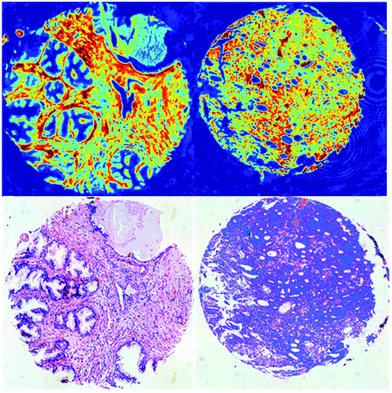
Successful exploitation of discrete frequency chemical imaging for high-throughput disease diagnosis requires the intelligent selection of salient frequencies that provide the greatest discriminatory power between diseased and healthy states. Failure to choose the correct wavenumbers could result in crucial spectral biomarkers being missed and could directly impact diagnostic accuracy. In addition, not all wavenumbers are suitable biomarkers and often provide little or no useful biochemical information. Acquiring too many wavenumbers increases measurement times and therefore reduces throughput. Numerous examples exist in the literature of well-established biomarkers^28,29 determined using FTIR chemical imaging. However, to date no studies have been performed on the transferability of biomarkers obtained using FTIR to discrete frequency IR spectroscopy. We have addressed this by acquiring full band spectra and subsequently identifying key biomarkers at sparsely located frequencies.

Chemical images were acquired in the spectral range 1000–1800 cm⁻¹ from tissue cores from two patients who had been diagnosed with prostate cancer. The first patient core was histologically classified as Normal-Associated Tissue (NAT) and contained normal tissue components only. The second patient core was classified as cancerous and contained morphological features consistent with a Gleason grade of 4. Since the cores available for the study had Gleason grades ranging between 3 and 5, choosing a core with a Gleason grade of 4 encompasses the middle of the cancer severity range. In principle, utilising a larger patient set for acquiring continuous infrared spectra would enable improved identification of the key wavenumbers. However, for the scope of this proof-of-concept study and due to the limited time available, we elected to choose a normal core and a cancerous core in the middle of the cancer severity range. Chemical images for each core based on the intensity of the amide I band are shown in Fig. 1.

Fig. 1 QCL chemical images of the amide I band intensity and H&E-stained serial section (bottom) for normal-associated tissue (left) and cancerous tissue (right) used to identify the key wavenumbers for discrete frequency classification.

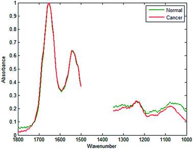
Employing similar methods as Fernandez,²⁰ a database was constructed consisting of 5000 spectra each for cancerous epithelium and normal-associated epithelium. The spectra were quality tested, truncated between 1350 and 1500 cm⁻¹ (to remove spectral regions describing bands of paraffin), and normalised to the amide I band. Mean spectra of the normal-associated and cancerous epithelium tissue are displayed in Fig. 2. Upon first inspection the spectra appear relatively similar, although some subtle differences can be discerned between 1000 and 1300 cm⁻¹.

Fig. 2 Mean spectra for normal-associated epithelium and cancerous epithelium from the database constructed from two prostate tissue cores, following truncation to remove the spectral regions describing wax, and normalisation to the 1652 cm⁻¹ band.

Half of the spectra from each class were selected at random and fed into a random forest³⁰ algorithm (software available from http://code.google.com/p/randomforest-matlab/). Random forests have the advantage that, unlike other supervised classifiers, they do not require feature selection prior to use. A random forest will return a measure for variable importance and identify the most important wavenumbers for classification. Alternative methods for wavenumber selection are available, such as partial least squares discriminant analysis (PLS-DA) and variable importance for projection (VIP), as described by Lloyd.³¹ The classifier was trained using 500 trees, with the number of wavenumbers selected at random to try and split each node (mtry) set to 2. The remainder of spectra in the database that had not been used for training were used to test the model.

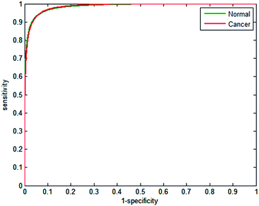
Receiver operator curves present an effective way to visualise the performance of the classifier. Each tree votes to classify a spectrum to a specific class, and the number of votes provides a probability estimate to each spectrum belonging to a particular class. Varying the probability acceptance thresholds adjusts the trade-off between sensitivity and specificity and produces a receiver operator curve (ROC). The ROCs obtained using the random forest classifier are displayed in Fig. 3.

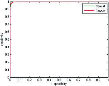Fig. 3 Receiver operator curves for normal and cancerous epithelium spectra using 2500 from each class for training and testing. AUC = 0.9991.

The optimal situation would be for curves to be situated at the top left hand corner of the plot, which indicates both high sensitivity and high specificity. Conversely, a poor classifier would be shown as a plot close to a diagonal line between the origin and top right corner. Area under the curve (AUC) is a widely accepted measure of classifier performance. The AUC for the plot shown in Fig. 3 is 0.991, demonstrating high performance of the classifier. Setting a probability of acceptance threshold of 0.5 enables a confusion matrix to be calculated and the ability to determine the proportion of each class that is correctly classified. Table 1 shows that normal-associated epithelium spectra are correctly classified with an accuracy of 97.25%, and cancerous epithelium with an accuracy 97.19%.

Table 1 Confusion matrix showing classification accuracy for normal-associated and cancerous epithelium using the random forest classifier with 500 trees

	Normal	Cancer
Normal	97.25	2.25
Cancer	2.81	97.19

---

Wavenumbers were then ranked in order of variable importance using a GINI importance plot to determine which were most important in distinguishing between normal and cancerous epithelium. Fig. 4a and b show typical GINI plots used to select the 25 most important features. The top 25 wavenumbers from a single GINI plot were selected for data collection. Subsequent repetition of the analysis shows that the first 14 wavenumbers are consistently in the top 16, but the remaining 11 wavenumbers selected can be ranked as far down as 58. This is not too surprising given that the difference in importance starts to drop off significantly after 20.

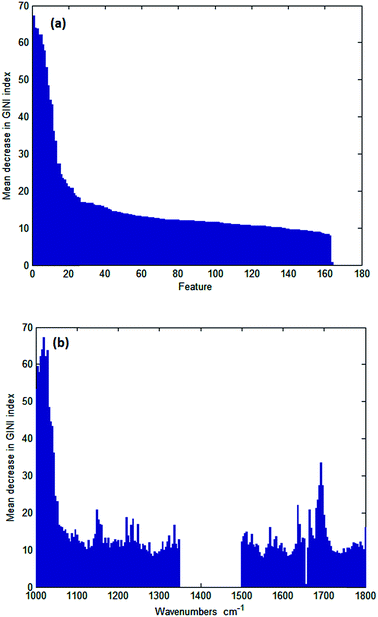Fig. 4 GINI importance plot (a) as a function of wavenumber and (b) ranked in order of variable importance.

The twenty five discriminating wavenumbers that were originally used in order of variable importance are shown in Table 2. The selected wavenumbers broadly overlap absorption bands centred at 1032 cm⁻¹ν (C–O) glycogen, 1080 cm⁻¹ν_s (PO₂⁻), 1236 cm⁻¹ν_as (PO₂⁻), 1540 cm⁻¹ (amide II), and 1656 cm⁻¹ (amide I).

Table 2 25 key wavenumbers (cm⁻¹) ranked in order of variable importance, as identified by the random forest classifier. Figures in parentheses indicate the variable importance ranking, with the lowest number being the highest ranking

Wavenumber (cm^−1)
(1) 1024	(2) 1020	(3) 1028	(4) 1016	(5) 1012	(6) 1072	(7) 1000	(8) 1004
(9) 1032	(10) 1636	(11) 1068	(12) 1088	(13) 1684	(14) 1092	(15) 1008	(16) 1640
(17) 1688	(18) 1692	(19) 1064	(20) 1648	(21) 1236	(22) 1696	(23) 1096	(24) 1524
(25) 1044

---

3.2 Discrete frequency imaging and classification

Discrete frequency chemical images were acquired from each of the 50 prostate tissue biopsy cores. Two wavenumbers at 1652 cm⁻¹ and 1734 cm⁻¹ in addition to the twenty five key wavenumbers (Table 2) were also acquired. The difference in absorbance at these two wavenumbers enabled the height of the amide I band to be determined, and this was used to quality check the spectra with spectra having an amide I intensity of between 0.1–2 being retained. Fig. 5 shows chemical images from a single prostate tissue core based on the intensity of the 1652 cm⁻¹, 1524 cm⁻¹, and 1236 cm⁻¹ bands and the H&E-stained serial section. The chemical images shown have been quality tested and spectra with amide I peak absorbance intensity between 0.1 and 2.0 retained. The image illustrates that rapid chemical imaging using discrete frequencies enables different types of tissue to be highlighted depending on the chosen frequency. Chemical images obtained at 1652 cm⁻¹ and 1524 cm⁻¹ enable differentiation between epithelium and stroma, while the 1236 cm⁻¹ chemical image highlights regions of stroma.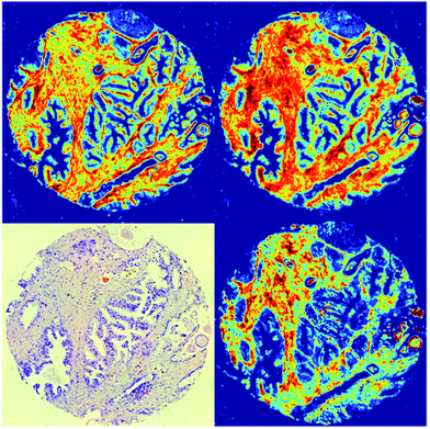

Fig. 5 Discrete frequency chemical images of a prostate tissue single core obtained using (clockwise from top left) 1652 cm⁻¹, 1524 cm⁻¹, and 1236 cm⁻¹ band intensity and H&E-stained serial section.

Chemical images from each of the 50 cores were compared to the corresponding H&E-stained serial sections to identify regions of cancerous and normal-associated epithelium. The patients were then randomly divided into two separate libraries to form a training cohort (15 patients) and a testing cohort (14 patients). The patients in each cohort were fairly evenly distributed across the two separate TMA slides. The training cohort had a split of 8 patients on one slide and 7 on the other. While the testing cohort was split with 8 patients on one slide and 6 on the second slide. Using the methods previously described by Fernandez,²⁰ two spectral databases were constructed from these cohorts, consisting of a training data set and an independent test set. Dividing the patients (and the data) prior to building the classifier ensures that the test set is completely independent, since no spectra used in training the model will be used for testing. Equal numbers of spectra from each class (normal-associated and cancerous epithelium) were extracted from the training database. Spectra were quality tested, baseline corrected and normalised to the amide I band. The mean cancerous epithelium and normal epithelium spectra based on 207 505 measurements each are shown in Fig. 6. Despite the limited number of data points in each spectrum, subtle spectral differences between the two classes are discernible, particularly between 1000 and 1240 cm⁻¹.

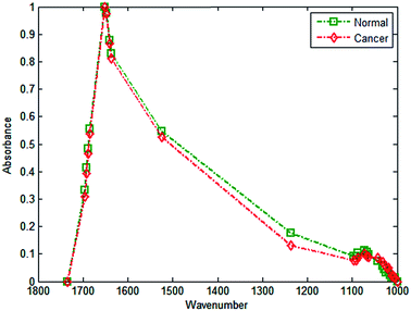Fig. 6 Discrete frequency mean spectra utilising 27 wavenumbers for cancerous and normal-associated epithelium. Dashed lines are present as a guide to the eye.

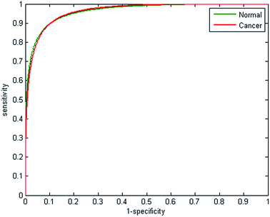
Half the spectra contained in the training database were randomly selected to train the model, with the remainder forming a validation test set. Metrics fed into the classifier were based on the absorbance values for each of the 25 discrete frequencies, and also all possible ratio combinations for the discrete frequency dataset, which yielded 325 features in total. The random forest classifier was then trained on the 207 505 partitioned spectra using 200 trees, which enabled the classifier to be constructed in approximately 90 minutes. The remaining spectra in the training data base were used to validate the model. The receiver operator curves obtained are displayed in Fig. 7. AUC values for the classifier are close to 1 (0.9895), indicating that the classifier can easily differentiate between normal and cancerous epithelium spectra. Despite utilising only 25 wavenumbers, the correctness of classification is high, with sensitivity and specificity of 93.39% and 94.72% respectively, as shown by the confusion matrix in Table 3.

Fig. 7 Receiver operator curves (ROC) with 25 wavenumbers (325 features), using validation data for normal-associated and cancerous epithelium. Area under the curve values (AUC) are normal = 0.9851, cancer = 0.9851.

Table 3 Confusion matrix showing correctness of classification using 25 wavenumbers for normal and cancerous epithelium

	Normal	Cancer
Normal	93.39%	6.61%
Cancer	5.28%	94.72%

---

The large number of features used to train the random forest classifier, and the substantial size of the data set, are the main factors responsible for lengthy training times. In an attempt to speed up training, the classifier was also trained using only the absorbance values at each of the 25 discrete frequencies. Training using 207 505 spectra per class using 200 trees enabled the random forest classifier to be constructed in just 8 minutes. The ROCs obtained using 25 features are shown in Fig. 8. The reduction in the features used in training has an impact on the performance of the classifier, the AUC decreasing from 0.9895 to 0.9625. Furthermore the sensitivity and specificity decreases to 89.14% and 90.32% respectively, suggesting that despite the increased processing times, using 325 features constructed from the 25 discrete frequencies is more effective.

Fig. 8 Receiver operator curves (ROC) with 25 wavenumbers (25 features), using validation data for normal-associated and cancerous epithelium. Area under the curve values (AUC) are normal = 0.9625, cancer = 0.9625.

The training data was then subjected to repeated random sub-sampling validation using ten repeats. In each case half the spectra in the database were randomly selected and used for training, while the remainder served as validation spectra. Table 4 shows the mean and standard deviation for the calculated sensitivity and specificity of the ten classifiers trained. The mean sensitivity and specificity from the repeated sub-sampling is high and provides a very small standard deviation, indicating that the classifier accuracy is not dependent on the spectra used to train and test the model.

Table 4 Mean and standard deviation of sensitivity and specificity, obtained using repeated random sub-sampling validation of ten trained classifiers

	Sensitivity	Specificity
Mean	94.60%	93.39%
Standard deviation	0.0012	0.0010

---

3.3 Discrete frequency classification with restricted numbers of wavenumbers

While it is evident that 25 discrete wavenumbers allows good classification accuracy on the validation data set, the effect of the number of discrete wavenumbers measured on classification accuracy is a key question. Clinical translation of discrete frequency infrared imaging requires high-throughput, high-resolution imaging utilising as few discrete wavenumbers as possible. Naturally, there will be a trade-off between the number of wavenumbers acquired and the classification accuracy. We have addressed this by reducing the number of wavenumbers used to train the model. We elected to reduce the number of wavenumbers used in classification rather than re-measuring all the cores with the respective number of wavenumbers due to time considerations and the desire for better comparability. In each case the subset of wavenumbers used was those with the highest variable importance values (Table 2), to ensure optimal classifier performance. Six separate experiments were performed on the training database using varying numbers of discrete wavenumbers. Table 5 details the discrete wavenumbers used for training and validating the random forest classification model.

Table 5 Discrete wavenumbers used for training the classifier with 20, 18, 16, 14, 12, and 10 different wavenumbers

Number of discrete wavenumbers	Discrete wavenumbers (cm^−1) used for random forest classification
20	1024	1020	1028	1016	1012	1072	1000	1004	1032
	1636	1068	1088	1684	1092	1008	1640	1688	1692
	1064	1648
18	1024	1020	1028	1016	1012	1072	1000	1004	1032
	1636	1068	1088	1684	1092	1008	1640	1688	1692
16	1024	1020	1028	1016	1012	1072	1000	1004	1032
	1636	1068	1088	1684	1092	1008	1640
14	1024	1020	1028	1016	1012	1072	1000	1004	1032
	1636	1068	1088	1684	1092
12	1024	1020	1028	1016	1012	1072	1000	1004	1032
	1636	1068	1088
10	1024	1020	1028	1016	1012	1072	1000	1004	1032
	1636

---

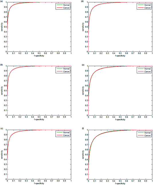
The performance of each classifier is shown in the ROCs in Fig. 9(a–f). Decreasing the number of wavenumbers used in classification reduces the performance of the classifier, as observed in the AUC values of 0.9780 and 0.9739 for 20 and 18 wavenumbers respectively. Reducing the number of discrete frequencies is expected to reduce classifier performance, since less information is being used during training. Surprisingly, training the random forest with just 18 wavenumbers still enables excellent discrimination between normal-associated and cancerous epithelium tissue. Reducing the numbers of wavenumbers further to 16 discrete frequencies only has a marginal effect on classifier performance (AUC = 0.9772). However, when using 12 or 10 discrete frequencies, the classifier performance begins to deteriorate with AUC values of 0.9557 and 0.9421 respectively.

Fig. 9 Receiver operator curves using validation data for normal-associated and cancerous epithelium with (a) 20, (b) 18, (c) 16, (d) 14, (e) 12 and (f) 10, discrete frequencies. AUC values are 0.9780, 0.9739, 0.9720, 0.9669, 0.9557 and 0.9421 respectively.

AUC values provide a good comparison of classification accuracy, however a more meaningful measure is the proportion of correctly classified spectra. Table 6 shows the proportion of correctly classified cancerous (sensitivity) and normal-associated epithelium (specificity) as a function of the discrete frequencies used in classification. The values for sensitivity and specificity are the mean values based on repeated random sub-sampling using ten repeats.

Table 6 Table showing sensitivity and specificity for the validation data using random subset sampling using ten repeats

Number of discrete frequencies	25	20	18	16	14	12	10
Sensitivity (%)	94.60	93.02	92.27	91.88	91.13	89.11	87.15
Specificity (%)	93.39	91.71	91.16	91.03	90.05	88.53	86.80

---

The sensitivity and specificity are broadly in line with the AUC values, and using all 25 wavenumbers enables high classification accuracy. Reducing the number of discrete frequencies to 16 still results in good classification accuracy with sensitivity and specificity of 91.88% and 91.03% respectively. Performance of the classifier becomes poorer when using 12 or fewer discrete frequencies. However using only 10 wavenumbers still enables surprisingly good classification accuracy, with sensitivity and specificity of 87.15% and 86.80%. Inspection of Table 5 reveals that, when using 10 discrete frequencies, the majority of the wavenumbers are in the range 1000–1072 cm⁻¹, indicating that important spectral biomarkers are located here.

The number of discrete frequencies chosen when acquiring chemical images is a key parameter. However, the time penalty associated with collecting increasing numbers of discrete frequencies is also an important consideration. Furthermore, as the number of discrete frequencies increases, so does the time required to train the random forest classifier. The performance of the random forest classifier as a function of AUC, sensitivity, specificity, acquisition time per core, and training time are shown in Table 7.

Table 7 Table showing AUC, sensitivity, specificity, collection time per core, and classifier training time as a function of the number of discrete frequencies used with the random forest classifier

No. of frequencies	AUC	Sensitivity	Specificity	Collection time per core (min)	Training time (min)
25	0.9851	94.60	93.39	5.5	90
20	0.9780	93.02	91.71	4.47	60
18	0.9739	92.27	91.16	4.33	48
16	0.9772	91.88	91.03	4.13	37
14	0.9669	91.13	90.05	4	32
12	0.9557	89.11	88.53	3.6	24
10	0.9421	87.15	86.80	3.27	17

---

The resulting sensitivity and selectivity are excellent when using the full 25 discrete frequencies, and a single core can be measured in 5.5 minutes, which is a reasonable timescale. However, constructing the classifier takes the longest time at ca. 90 minutes. Utilising only 10 discrete frequencies enables fast data acquisition (3.27 minutes), and the random forest classifier can be constructed in just 17 minutes. However, the improved throughput and analysis time is offset by the reduced sensitivity and specificity of 87.15% and 86.80% respectively. To put this into perspective it is crucial to understand what timescales would be clinically acceptable. Once the classifier has been trained and robustly validated there would not be a requirement to retrain the classifier on a regular basis. Therefore, provided that the classifier can be trained within reasonable timescales, then the key parameter is the collection time per core. Utilising between 14 and 16 discrete frequencies enables each core to be measured in approximately 4 minutes while maintaining sensitivity and specificity >90%. Although there is a slight reduction in sensitivity and specificity compared to utilising the full 25 discrete frequencies, there is a considerable time saving of approximately 90 seconds per core. We would suggest that acquiring high-resolution images of a single TMA acquired in just four minutes, while maintaining high sensitivity and specificity, would be clinically acceptable.

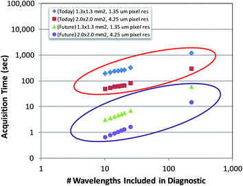
As QCL-based, full-field imaging technology continues to advance over the coming years, this tradeoff will become less apparent to the clinician. The underlying technology employed in this work is scalable and has the potential to reach data collection times 1–2 orders of magnitude shorter, limited by the thermal time constant of the bolometer (typically 0.33/fps) and the time required to step the stage a single FOV when building mosaic images. Even today, if a slightly lower pixel resolution of 4.25 μm is deemed acceptable for the application, a 9.5× increase in throughput could be achieved simply by using the 0.3 NA 4× objective with a 2 mm × 2 mm FOV. In this configuration, tissue cores with diameters up to 2 mm could be imaged in a quarter of the times reported in this work. Current and expected future trends in data acquisition times as a function of the number of discrete wavenumbers employed in the diagnostic for two different area–pixel resolution configurations are shown in Fig. 10.

Fig. 10 Data acquisition times vs. the number of discrete wavenumbers included in the diagnostic for the current and future QCL full-field imaging technology used in this work. Two different imaging configurations were used in this analysis: (1) 1.3 mm × 1.3 mm (2 × 2 mosaic) at 1.35 μm pixel size (this work), and 2.0 mm × 2.0 mm (single FOV) at 4.25 μm pixel size.

Estimating future throughput trends assumed two camera frames (at 30 fps) are used per discrete wavenumber to ensure adequate settling and 125 msec stage mosaic step times. Based on these results, it becomes immediately apparent that whole-slide diagnostic imaging could eventually be completed in a matter of minutes using the protocols developed in this work.

3.4 Discrete frequency classification: independent test set

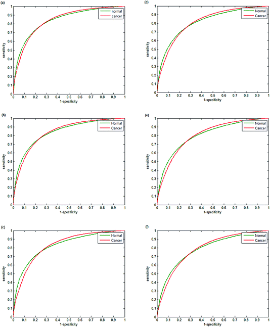
Testing classifier performance using the same patients for training and testing is likely to produce favourable results, since inter-patient variability does not become a factor. Implementation of SHP in the clinic requires that good classification of disease state can be achieved as new patients are introduced. Confidence in SHP using discrete frequency imaging can only be achieved if it performs well on patients in an independent test set. Each random forest classifier was used to classify epithelium spectra from the 14 patients in the independent test set. The ROCs obtained in each case are shown in Fig. 11(a–f) and 12. Fig. 11(a) shows the ROC obtained when using 25 discrete frequencies for training and classification on the independent test set. The AUC values that were obtained for the validation set were observed to be all close to 1, indicating good discrimination between classes when training and testing occurs on the same patients. However, testing the classifier on the independent test set reduces the AUC values from 0.9851 for the validation data to 0.8395 for the independent test set. Reduced classification accuracy is expected to occur for the independent test, since the data used to test the model are from new patients and therefore completely independent. Reducing the number of discrete frequencies decreases AUC values for the independent test set, in a similar manner observed for the training data set. The AUC value of 0.8396 obtained using 20 discrete frequencies instead of 25 (0.8395) is very similar, indicating that classification performance has not deteriorated significantly. Although there is a slight reduction in AUC (0.8163) when using 16 wavenumbers, each ROC plot appears broadly similar. Classification performance only appears to deteriorate significantly when utilising 14 or fewer discrete frequencies. Using only 10 discrete frequencies (Fig. 12), the AUC value decreases to 0.7808, which is in stark contrast to the validation set, which had an AUC value of 0.9421.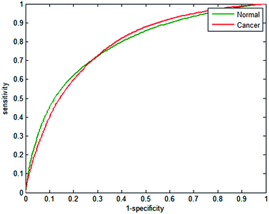

Fig. 11 Receiver operator curves using the independent test set for normal-associated and cancerous epithelium with (a) 25, (b) 20, (c) 18, (d) 16, (e) 14, and (f) 12 discrete frequencies. AUC values are 0.8395, 0.8396, 0.8261, 0.8163, 0.8044 and 0.7876 respectively.

Fig. 12 Receiver operator curves (ROC) with 10 wavenumbers using independent test set for normal-associated and cancerous epithelium. Area under the curve (AUC) values are 0.7808.

The effect of reducing the number of discrete frequencies on sensitivity and specificity is shown in Table 8. Utilising the full 25 discrete frequencies enables reasonable classification accuracy rates of 72.14% and 80.23% for sensitivity and specificity respectively. Reducing the number of discrete frequencies to 16 only has a limited impact on classification, with sensitivity and specificity values of 70.46% and 78.10%. In contrast to the validation set, the sensitivity does not appear to deteriorate significantly when reducing the number of discrete frequencies. Specificity, however, does appear to be strongly correlated to the number of discrete frequencies, and performance drops off sharply when less than 14 wavenumbers are used. When using only 10 wavenumbers the classification of the independent test set is poorer, with a mean sensitivity and specificity of 68.73% and 73.51% respectively.

Table 8 Table showing sensitivity and specificity for the independent test set using random subset sampling for ten trained classifiers

Discrete frequencies	25	20	18	16	14	12	10
Sensitivity (%)	72.14	71.29	71.13	70.46	69.48	68.25	68.73
Specificity (%)	80.23	80.83	78.86	78.10	76.69	75.07	73.51

---

The poorer performance of the classifiers on the independent test set is surprising considering the excellent classifier performance using the training data. Since all patients in this study have been diagnosed with prostate cancer, there is likely to be considerable biochemical variability between patients. To perform well on new patients, the model needs to be trained on a dataset that encompasses this variation. Given the limited patient numbers available in this study for training and testing, it is likely that the model did not have sufficient variability built in to enable good discrimination between normal and cancerous tissue for new patients. Similar findings have been published by Pounder³² when using spectral histology of breast tissue using FTIR chemical imaging. In their study, good classification performance was observed on the training data for classifying epithelium, lymphocytes and myofibroblast-rich stroma with AUC values of 0.94. Upon classifying an independent test set there was a deterioration in classifier performance, with AUC values in the range of 0.8–0.88. The authors described this effect as being due to the limited number of cores (50) and patients used in the study. These findings are broadly in line with the classifier performance which we have detailed in this paper. We have also considered whether instrumental or sample preparation parameters could be a contributory factor to the poorer classification accuracy of the independent test set. Variability in sample and substrate thickness, and whether the samples are left in wax or dewaxed are all parameters that could potentially affect classifier performance. However, a much larger study investigating the effect of each parameter will be required to determine the optimum parameters for classification performance. Another possibility for the poorer classification on the independent test set is the selection of the salient spectral frequencies. In this proof-of-concept study only two patients were used for selecting the spectral frequencies used to train and test the model. Given the biochemical variability within a patient population, it is unlikely that two patients are a sufficiently large dataset for identifying the key biomarkers. In the future it is recommended that a larger patient population is used for frequency collection, and this is planned to be conducted. Although our preliminary results are promising, larger studies using a more diverse patient database would be required to fully evaluate the full potential of discrete frequency imaging for disease diagnosis.

4 Conclusions

Discrete frequency infrared chemical imaging has the potential to provide high-resolution, high-throughput chemical images on a timescale that could revolutionise spectral histopathology. In this study, we have demonstrated that high-quality chemical images of tissue biopsy cores composed of almost a million pixels can be obtained in a matter of minutes. Comparable chemical images obtained on a state-of-the-art FTIR system using an FPA detector would have taken several hours. We have clearly demonstrated on a validation set that excellent classifier performance can be achieved by careful selection of discrete frequencies. We have further shown that significant time advantages can be achieved by using just 16 discrete frequencies while maintaining good classification accuracy. Testing the classifier on an independent test set produced mixed results, with poorer accuracy than on the validation set. However, reasonable classification accuracy could still be achieved when using 16 or more discrete frequencies. Classifier performance may have been compromised by only using two patients for selecting the optimal wavenumbers. Utilising a larger patient population for determining the key biomarkers will be important in any future studies. Limitations on the number of patient tissue core biopsy samples available are the most likely cause of the reduced accuracy when testing on new patients. Prospects for this new and exciting technology are bright. However, further work needs to be performed on significantly larger patient numbers to fully understand its potential for successful implementation in the clinic.

Acknowledgements

We would like to thank Daylight Solutions for making the Spero infrared microscope available to us for the duration of the study. We would also like to acknowledge Jeremy Rowlette, Edeline Fotheringham, Miles Weida, Bill Mohar and Matthew Barre for their help on the project and also for their roles during informative discussions. PG and MP would like to acknowledge the EPSRC for funding (EP/K02311X/1, EP/L012952/1).

Notes and references

1. L. G. Luna, Manual of Histologic Staining Methods of the Armed Forces Institute of Pathology, McGraw Hill, New York, 1968.
2. W. P. Michael and H. Ross, Histology a text and atlas, Lippincott Williams & Wilkins, 6th edn, 2010.
3. J. B. Lattouf and F. Saad, BJU Int., 2002, 90, 694–698 , discussion 698–699.
4. H. Fabian, P. Lasch, M. Boese and W. Haensch, Biopolymers, 2002, 67, 354–357.
5. B. R. Wood, L. Chiriboga, H. Yee, M. A. Quinn, D. McNaughton and M. Diem, Gynecol. Oncol., 2004, 93, 59–68.
6. B. Bird, M. Miljkovi, S. Remiszewski, A. Akalin, M. Kon and M. Diem, Lab. Invest., 2012, 92, 1358–1373.
7. N. Bergner, B. F. M. Romeike, R. Reichart, R. Kalff, C. Krafft and J. Popp, Analyst, 2013, 138, 3983–3990.
8. M. J. Baker, E. Gazi, M. D. Brown, J. H. Shanks, N. W. Clarke and P. Gardner, J. Biophotonics, 2009, 2, 104–113.
9. A. Akalin, B. Bird, X. Mu, M. A. Kon, A. Ergin, S. H. Remiszewski, C. M. Thompson, D. J. Raz and M. Diem, Lab. Invest., 2015, 95, 406–421.
10. E. Gazi, M. Baker, J. Dwyer, N. P. Lockyer, P. Gardner, J. H. Shanks, R. S. Reeve, C. A. Hart, N. W. Clarke and M. D. Brown, Eur. Urol., 2006, 50, 750–761.
11. N. Wald and E. Goormaghtigh, Analyst, 2015, 140, 2144–2155.
12. K. M. Dorling and M. J. Baker, Trends Biotechnol., 2013, 31, 437–438.
13. M. J. Walsh, D. Mayerich, A. Kajdacsy-Balla and R. Bhargava, 2012.
14. A. Liu, L. Wei, W. A. Gardner, C.-X. Deng and Y.-G. Man, Int. J. Biol. Sci., 2009, 5, 276–285.
15. P. R. Pandey, J. Saidou and K. Watabe, Front. Biosci., 2010, 15, 226–236.
16. M. J. Walsh, S. E. Holton, A. Kajdacsy-Balla and R. Bhargava, Vib. Spectrosc., 2012, 60, 23–28.
17. L. S. Leslie, A. Kadjacsy-Balla and R. Bhargava, Medical Imaging: Digital Pathology, 2015, 9420.
18. P. Bassan, J. Mellor, J. Shapiro, K. J. Williams, M. P. Lisanti and P. Gardner, Anal. Chem., 2014, 86, 1648–1653.
19. R. Bhargava, Anal. Bioanal. Chem., 2007, 389, 1155–1169.
20. D. C. Fernandez, R. Bhargava, S. M. Hewitt and I. W. Levin, Nat. Biotechnol., 2005, 23, 469–474.
21. H. Brooke, B. V. Bronk, J. N. McCutcheon, S. L. Morgan and M. L. Myrick, Appl. Spectrosc., 2009, 63, 1293–1302.
22. J. Filik, M. D. Frogley, J. K. Pijanka, K. Wehbe and G. Cinque, Analyst, 2012, 137, 853–861.
23. P. Bassan, J. Lee, A. Sachdeva, J. Pissardini, K. M. Dorling, J. S. Fletcher, A. Henderson and P. Gardner, Analyst, 2013, 138, 144–157.
24. M. J. Pilling, P. Bassan and P. Gardner, Analyst, 2015, 140, 2383–2392.
25. P. Bassan, A. Sachdeva, J. H. Shanks, M. D. Brown, N. W. Clarke and P. Gardner, 2014, 9041, 90410D.
26. M. J. Baker, J. Trevisan, P. Bassan, R. Bhargava, H. J. Butler, K. M. Dorling, P. R. Fielden, S. W. Fogarty, N. J. Fullwood, K. A. Heys, C. Hughes, P. Lasch, P. L. Martin-Hirsch, B. Obinaju, G. D. Sockalingum, J. Sulé-Suso, R. J. Strong, M. J. Walsh, B. R. Wood, P. Gardner and F. L. Martin, Nat. Protoc., 2014, 9, 1771–1791.
27. P. Bassan, M. J. Weida, J. Rowlette and P. Gardner, Analyst, 2014, 139, 3856–3859.
28. Y. Yang, J. Sulé-Suso, G. D. Sockalingum, G. Kegelaer, M. Manfait and A. J. El Haj, Biopolymers, 2005, 78, 311–317.
29. E. Gazi, J. Dwyer, P. Gardner, A. Ghanbari-Siahkali, A. P. Wade, J. Miyan, N. P. Lockyer, J. C. Vickerman, N. W. Clarke, J. H. Shanks, L. J. Scott, C. A. Hart and M. Brown, J. Pathol., 2003, 201, 99–108.
30. L. Breiman, Journal of Machine Learning, 2001, 45, 5–32.
31. G. R. Lloyd and N. Stone, Appl. Spectrosc., 2015, 69, 1066–1073.
32. F. N. Pounder and R. Bhargava, 2009, vol 7182, p. 718206.

---