Quantitative ionization energies and work functions of aqueous solutions

Abstract

Despite the ubiquitous nature of aqueous solutions across the chemical, biological and environmental sciences our experimental understanding of their electronic structure is rudimentary—qualitative at best. One of the most basic and seemingly straightforward properties of aqueous solutions—ionization energies—are (qualitatively) tabulated at the water–air interface for a mere handful of solutes, and the manner in which these results are obtained assume the aqueous solutions behave like a gas in the photoelectron experiment (where the vacuum levels of the aqueous solution and of the photoelectron analyzer are equilibrated). Here we report the experimental measure of a sizeable offset (ca. 0.6 eV) between the vacuum levels of an aqueous solution (0.05 M NaCl) and that of our photoelectron analyzer, indicating a breakdown of the gas-like vacuum level alignment assumption for the aqueous solution. By quantifying the vacuum level offset as a function of solution chemical composition our measurements enable, for the first time, quantitative determination of ionization energies in liquid solutions. These results reveal that the ionization energy of liquid water is not independent of the chemical composition of the solution as is usually inferred in the literature, a finding that has important ramifications as measured ionization energies are frequently used to validate theoretical models that posses the ability to provide microscopic insight not directly available by experiment. Finally, we derive the work function, or the electrochemical potential of the aqueous solution and show that it too varies with the chemical composition of the solution.

---

Introduction

The ability to predict and to understand chemical reactions, hydration structures and charge transfer processes in aqueous solutions is governed by the electronic structure of the liquid. Arguably the most sought components in this regard are the ionization energies (IE) of the solvent (water) and solute orbitals^1–9 as their energies dictate whether single electron transfers between different species in solution are possible.¹⁰

Ionization energies of aqueous solutions are measured by photoelectron spectroscopy (PES) using a liquid jet;⁸ however, published values for the same, or similar solution often differ substantially between laboratories,^11–14 or even within a single laboratory.^15,16 This creates a less than satisfactory situation, as these experimental results are frequently used to validate theoretical models that posses the ability to provide microscopic insight not directly available by experiment.^9,17

To date, IEs of aqueous solutions determined by liquid jet PES using (synchrotron) soft X-ray radiation rely on two assumptions: (1) the aqueous solution behaves like a gas during the experiment, and (2) the ionization energy of liquid water is independent of the chemical composition of the solution. The former implies the vacuum levels of the aqueous solution and of the analyzer are equilibrated during measurement, while the latter, which appears surprising based on chemical intuition, simplifies the interpretation of the experimental result by providing an internal energy reference that enables for a spectral shift (for instance if the photon energy is not properly calibrated, or if the solution is charging during ionization)—analogous to using the inner shell 1s energy level of adventitious carbon as reference during a solid state PES experiment. In this approach, IEs of solutes in aqueous solutions measured with soft X-ray radiation are determined exclusively by referencing their energy to those of water, the latter are assumed independent of solute and solute concentration. Here, by measuring photoelectron spectra while applying external bias to the liquid jet we quantify the vacuum level offset of the aqueous solution. We show (i) that the vacuum levels of an aqueous solution and the photoelectron analyzer are not equilibrated during a PES experiment, and (ii) that the ionization energy of liquid water depends (strongly) on the chemical composition of the solution. These results unambiguously reveal that the two assumptions invoked a priori to interpret PES measurements from aqueous solutions using soft X-ray radiation are not universally valid and may introduce errors in the reported ionization energies. Quantitative ionization energies from an aqueous solution are only realized after accounting for the vacuum level offset between the solution and the photoelectron analyzer, something heretofore never reported. From the vacuum level offset we derive the work function (electrochemical potential) of the aqueous solution and show that it too varies substantially with the chemical composition of the solution.

Ionization energies from photoelectron spectroscopy

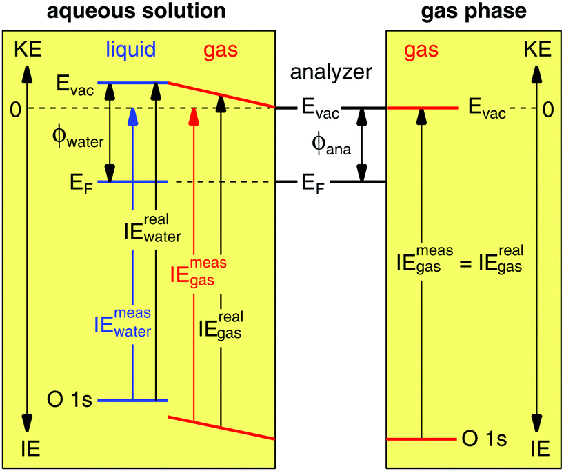
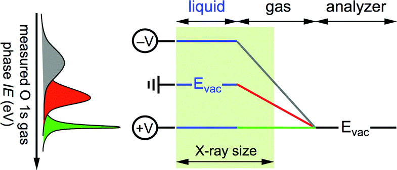
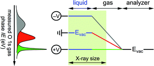
Gas phase water has a well-known IE^18,19 that can be measured by PES,

IE^meas_gas = hν − KE, (1)

where hν is the photon energy and KE the measured kinetic energy of the photoelectron. Zero KE is defined at the vacuum level of the analyzer. The measurement is straightforward to interpret in absence of any external influence because the vacuum level (E_vac) of the gas is equilibrated with that of the analyzer (Fig. 1, right hand side). In this case the measured ionization energy of the gas (IE^meas_gas) is also the real ionization energy (IE^real_gas), that is, the exact difference in energy between the occupied orbital under study and vacuum level of the gas.

Fig. 1 Energy level diagram for a gas phase (right hand side) and liquid jet of aqueous solution (left hand side) photoelectron spectroscopy experiment. Abbreviations: E_vac, vacuum level; E_F, Fermi energy; ϕ, work function; ana, analyzer; KE, kinetic energy; IE, ionization energy. In the gas phase experiment the vacuum level of the gas is equilibrated with that of the analyzer, whereas in the aqueous solution experiment the vacuum level of the gas is pinned to the vacuum levels of the liquid and of the analyzer, which results in an electric field between the two (depicted as sloped energy levels of the gas). Zero kinetic energy is defined for both experiments as the vacuum level of the analyzer.

Photoelectron spectroscopy from a liquid jet of aqueous solution combines a gas phase environment (the Knudsen layer of evaporating/condensing water molecules that surround the jet) with that of a (liquid) surface (Fig. 1, left hand side). The vacuum level of the gas is no longer equilibrated with that of the analyzer everywhere but is instead now pinned to both the vacuum levels of the analyzer and aqueous solution²⁰ with a linear gradient of the electric field between. The (liquid) surface and the analyzer are equilibrated through their Fermi energies, ensured during the PES experiment by measuring only conductive solutions that are in electrical contact with the analyzer (the liquid is grounded with the analyzer). The real ionization energies of the aqueous solution are given by,

IE^real_water = hν − KE + (ϕ_water − ϕ_ana), (2)

in absence of a streaming potential where ϕ_water and ϕ_ana are the work functions of the aqueous solution and analyzer, respectively, and zero KE is again defined at the vacuum level of the analyzer. The measured ionization energies—those reported in the literature under the assumption the vacuum level, and not the Fermi energy of the aqueous solution is equilibrated with the analyzer—are given by,

IE^meas_water = hν − KE, (3)

which deviates from the real value by the vacuum level offset (ϕ_water − ϕ_ana). While eqn (2) is straightforward to interpret, it requires quantifying the vacuum level offset between an aqueous solution and the analyzer, something heretofore never reported. Without accounting for this offset, IEs for the same aqueous solution will vary between laboratories (as is evident from the literature)^11–16 because KE depends on the vacuum level of the analyzer used to record the spectra. This effect is evident from the example schematic energy diagram of Fig. 1, which depicts the case where the work function of the aqueous solution is greater than that of the analyzer [(ϕ_water − ϕ_ana) > 0]. Under these conditions IE^meas_water is lower than IE^real_water; however, because no adequate reference IEs exist in the literature for aqueous solutions this effect would not be immediately obvious to the experimenter. A quantifiable observable is IE^meas_gas, which under these conditions is also lower than IE^real_gas (for which adequate reference is available^18,19), because the gas resides in a gradient of the electric field that affects all its energy levels (vacuum level and O 1s core level equally, see Fig. 1).²⁰ One can, therefore, immediately determine if the work function of an aqueous solution is greater (IE^meas_gas < IE^real_gas) or smaller (IE^meas_gas > IE^real_gas) than that of the analyzer by comparing the IE of gas phase water in absence and in the presence of the aqueous solution surface. If the vacuum levels of the aqueous solution and analyzer are equilibrated, as is traditionally assumed for the interpretation of liquid jet PES measurements, then IE^meas_gas = IE^real_gas and IE^meas_water = IE^real_water.

Experimental observation of a vacuum level offset between an aqueous solution and the photoelectron analyzer

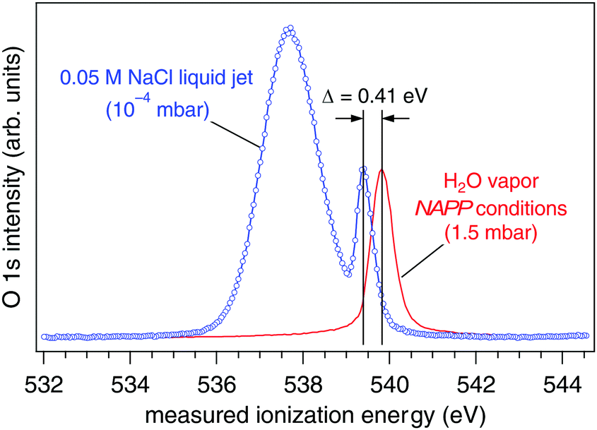
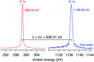
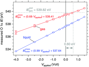
The ionization energy of the O 1s orbital of gas phase water is measured under near ambient pressure photoemission (NAPP) conditions at 1.5 mbar (Fig. 2, red trace). After calibrating the photon energy using hν and 2hν (see Experimental methods) we obtain the real ionization energy, IE^real_gas = 539.82(±0.02) eV, a result that agrees well with the literature.^18,19 Exchanging the NAPP conditions of the gas phase measurement for a liquid jet (0.05 M NaCl, 273 K) operating in 10⁻⁴ mbar, the O 1s core level spectrum reveals the presence of two well-resolved components (Fig. 2, blue trace). The more intense and significantly broader component at lower measured ionization energy (IE^meas_water = 537.64(±0.02) eV) corresponds, based on earlier assignments,²¹ to the aqueous solution of the liquid jet, whereas the component at higher ionization energy (IE^meas_gas = 539.41(±0.03) eV) is from gas phase water molecules that surround the liquid jet (the Knudsen layer). Based on the arguments set forth in the preceding section it becomes immediately clear from these two spectra that the work function of an aqueous solution of 0.05 M NaCl is greater than that of our analyzer because the measured gas phase O 1s IE is shifted lower in energy than its real value. As a consequence, all measured ionization energies from this aqueous solution (core and valence orbitals alike) will also be underestimated relative to their real values. In what follows we quantify the vacuum level offset between this 0.05 M NaCl aqueous solution and the analyzer using two different approaches with the goal of establishing (1) the real ionization energy and (2) the work function (electrochemical potential) of the aqueous solution. Results are then compared to those of a second aqueous solution, 0.15 M butylamine in 0.05 M NaCl.

Fig. 2 O 1s spectra of gas phase water under NAPP conditions at 1.5 mbar (red trace) and from a liquid jet of 0.05 M NaCl at 10⁻⁴ mbar (blue trace). The two components of the liquid jet spectrum originate from the liquid phase (lower ionization energy) and from gas phase water that surrounds the jet (Knudsen layer). The measured ionization energy of gas phase water shifts 0.41 eV lower in energy in the presence of the liquid jet. The spectra have been normalized in such a way that the two gas phase peaks have equal intensity.

Experimental methods

Gas phase ionization energy under NAPP conditions

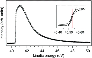
The ionization energy of the O 1s orbital of gas phase water is measured under near ambient pressure photoemission (NAPP) conditions. Triple-freeze–pump–thawed Milli-Q water is introduced inside the ionization chamber using a standard ultrahigh vacuum (UHV) leak value until a stable pressure of 1.5 mbar. During the measurement the vacuum system of the ionization chamber is switched off, however, there is small continuous pumping through the 500 μm aperture that serves as entrance to the differentially pumped electrostatic lens system of the analyzer. The UHV beamline is sealed from the ambient pressure of the ionization chamber by a 200 nm thick SiN_x membrane (Silson Ltd). The Scienta HiPP-2 spectrometer is operated in constant energy mode at pass energy of 100 eV using a curved entrance slit of 0.5 (width) × 25 (height) mm. The O 1s spectra regions (hν and 2hν) are collected using 0.05 eV energy steps of the analyzer. The ionization energy is calculated using eqn (1) after fitting the two spectra (Fig. 3) using Voigt functions.

Fig. 3 O 1s spectra from 1.5 mbar water vapour (in absence of any surface/liquid) using hν (left, red trace) and 2hν (right, blue trace). The ionization energy is calculated from eqn (1). The nominal photon energy of the beamline is 840.00 eV.

Liquid jet operation

X-ray photoelectron spectroscopy experiments are performed at the SIM beamline of the Swiss Light Source using the NAPP endstation²² and a 30 μm pinhole placed in the intermediate focus of the beamline that serves to reduce the X-ray spot size while also increasing the photon energy resolution of the beamline.²³ Fused quartz capillaries of 19 and 22 μm are used at 273 K (the solutions are passed through an ice bath immediately before entry to the ionization chamber) and with flow rates of 0.30 and 0.35 mL min⁻¹, respectively. A complete description of in situ PES from a liquid jet is given elsewhere.²¹ All experiments are performed in vacuum of 3–5 × 10⁻⁴ mbar by expanding the liquid jet to hit a LN₂-filled trap while continuously pumping the measurement chamber using an Agilent TwisTorr 700 turbo molecular pump backed by an Adixen Roots pump. The Scienta HiPP-2 spectrometer (referred to as analyzer throughout this article) is operated in constant energy mode at a pass energy of 100 eV. The entrance slit of the hemisphere is 0.3 (width) × 25 (length) mm (and curved), which results in a theoretical energy resolution better than 75 meV. The liquid jet is operated along the vertical length of the entrance slit. The titanium entrance cone of the analyzer has an aperture of diameter 0.5 mm. The working distance between the entrance cone and the liquid jet is 0.5 mm.

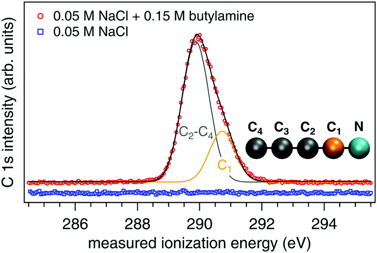
All aqueous solutions are prepared using Milli-Q water in glass bottles that are cleaned beforehand using a dilute Deconex 12 N-x solution and rinsed thoroughly with Milli-Q water. Before addition of the solutes, argon (Ar) gas is vigorously bubbled through the liquid water for 20 min. This ensures any dissolved CO₂ is removed, as verified by a measured pH of 7.0 (Mettler Toledo ExpertPro electrode, calibrated using a 4-point curve at pH 2.0, 4.01, 7.0 and 10.0). Sodium chloride (NaCl, ≥99.8%, ACS Reagent, Sigma-Aldrich) and 1-butylamine (99%, Alfa Aesar, C 1s spectrum in Fig. 4) are used as received. Once the aqueous solutions are prepared they are mounted to the high-pressure liquid chromatography (HPLC) pump used to supply the liquid jet and kept under constant purge by helium (He) throughout the experiments. This latter step was performed to ensure the solutions keep their native pH values and are not influenced by dissolved CO₂ from the atmosphere over the ∼16 h needed to perform one series of measurements.

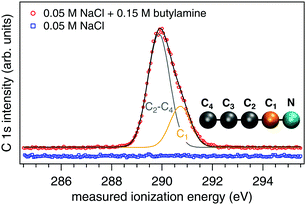Fig. 4 C 1s spectra from liquid jets of 0.05 M NaCl (blue trace) and 0.15 M butylamine in 0.05 M NaCl (red trace). The spectra are offset in intensity for clarity. The deconvolution of the butylamine spectrum into two components and their assignments are shown.

Our reference aqueous solutions are not pure water but instead contain 0.05 M NaCl. The C 1s spectrum of Fig. 4 from this solution shows that there is no trace of any carbon-based contaminants. Electrolyte is added to ensure sufficient conductivity to the liquid. 0.05 M NaCl is specifically chosen because it has been shown by experiments to largely suppress any streaming potential associated with the operation of the liquid jet.^12,24 Under these conditions, the streaming potential has been recently calculated to be only 6 mV,²⁵ a factor of more than six less than our smallest reported error (±40 mV) for a real ionization energy or work function of an aqueous solution. We therefore expect the ionization energies and work functions reported herein are not influenced by our use of a liquid jet. In addition, we have verified the conductivity of the solution is sufficient to suppress any potential charging caused by the X-ray beam by repeating the experiments using a factor of ca. five less photon flux (achieved by detuning the undulator of the beamline and estimating the flux using the current on the last refocusing mirror) with identical results.

External bias is applied to the liquid jet through a 225 μm gold wire mounted to the last metal (stainless steel) connection of the liquid jet (ca. 20 mm above the ionization point) using a Tektronix 60 V PWS4602 linear DC power supply with a resolution of ±1 mV. Spectra are fit using Voigt functions after a standard linear background subtraction.

Photon energy calibration

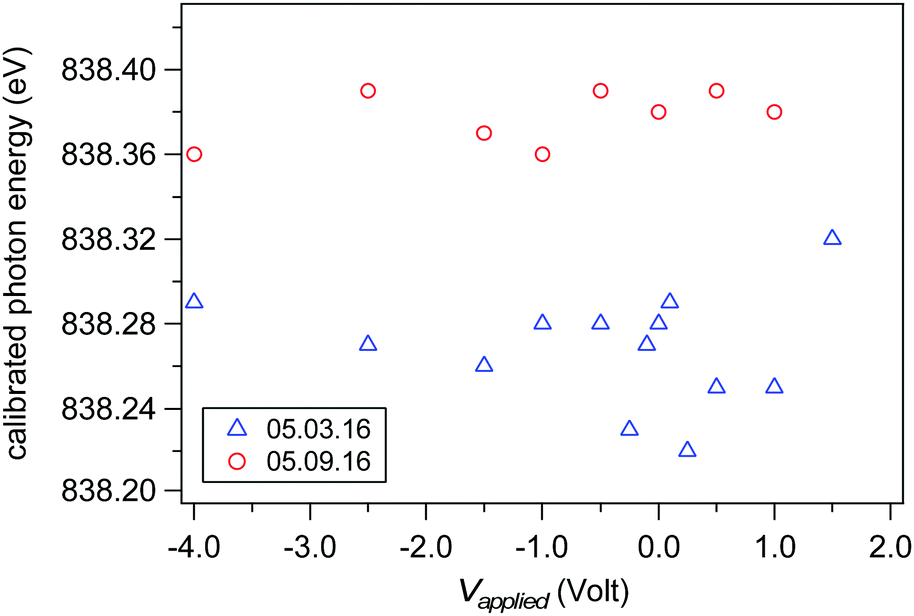
Accurate ionization energies are calculated only after the exact photon energy of the incident X-ray is determined. We have calibrated the photon energy during each scan reported in this article by simultaneously collecting the O 1s spectral region using photon energies hν and 2hν (see example in Fig. 3). The two O 1s spectral regions are then fit (with liquid and gas phase peaks) and the difference in kinetic energy between the O 1s liquid phase components set as the photon energy. Fig. 5 shows the calibrated beamline energy from scan-to-scan and day-to-day for all measurements from a liquid jet of 0.05 M NaCl (the spectra of Fig. 8 and the results of Fig. 9). The offset in photon energy of up to 0.15 eV between the different measurement day's may originate from small changes in orbit of the electron storage ring or from small temperature-dependent shifts in the energy slit position after the monochromator. These observed shifts highlight the importance of calibrating the photon energy during each scan if exact IEs are sought.

Fig. 5 Calibrated photon energy for each spectra of the 0.05 M NaCl series of data (the spectra of Fig. 8 and the results in Fig. 9). Calibration was done by measuring O 1s spectra from both hν and 2hν (see example spectra in Fig. 10). The nominal photon energy of the beamline was 840.00 eV. Results for measurements performed on two different days are shown in blue (May 3rd, 2016) and red (May 9th, 2016).

Work function of the analyzer

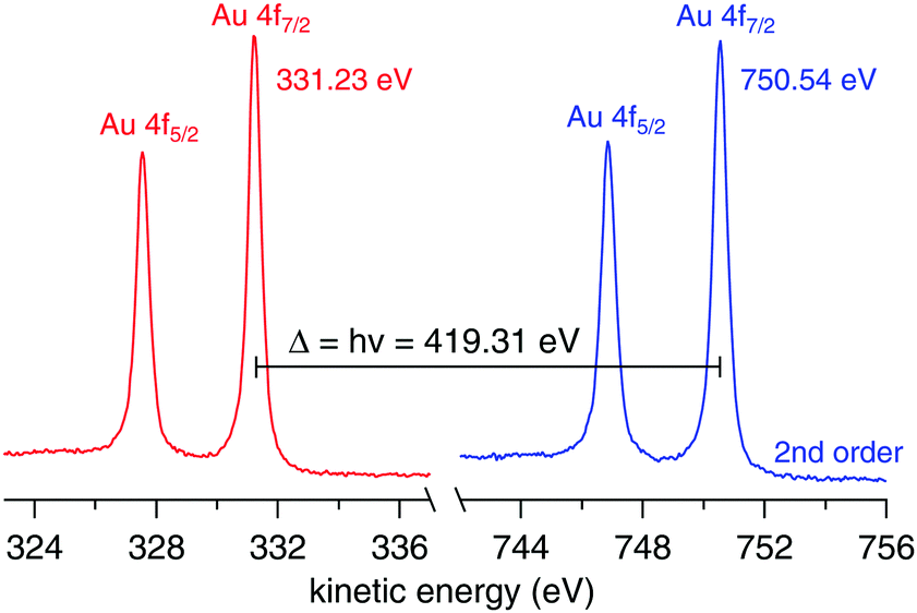
The work function of the analyzer is determined using a 100 μm gold wire mounted in place of the liquid jet. The work function is calculated using

ϕ_ana = hν − BE_Au4f − KE_Au4f, (4)

where hν is the calibrated photon energy, BE_Au4f the known binding energy of the Au 4f_7/2 peak, 84.00(±0.05) eV,²⁶ and KE_Au4f the measured kinetic energy of the Au 4f_7/2 peak. Fig. 6 shows the spectra used to calculate ϕ_ana = 4.08(±0.06) eV.

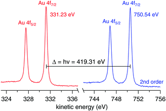Fig. 6 Au 4f spectra from a 100 μm gold wire mounted in place of the liquid jet using hν (left, red trace) and 2hν (right, blue trace). The nominal photon energy of the beamline was 420.00 eV.

Results and discussion

Quantifying the real ionization energy of an aqueous solution

The magnitude of the shift in the O 1s gas phase ionization energy observed in Fig. 2 depends not only on the vacuum level offset between the aqueous solution and the analyzer (ϕ_water − ϕ_ana), but additionally on a geometric factor, c, that is specific to the experimental setup.²⁷ This geometric factor accounts for the size of the ionization source sampling a finite gas volume somewhere between the liquid and the analyzer (Fig. 7). In this volume gas phase molecules experience a gradient in the electric field that affects their IEs to different extents depending on their distance from the liquid jets surface (recall that the origin of this electric field gradient is the vacuum level of the gas being pinned to both that of the aqueous solution and the analyzer, Fig. 1 and 7).²⁷ The difference between the real and measured O 1s gas phase IEs is given by,

IE^real_gas − IE^meas_gas = c(ϕ_water − ϕ_ana), (5)

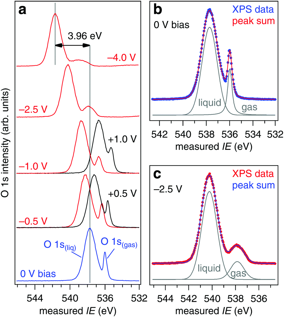
where IE^real_gas is measured in absence of the liquid jet (NAPP conditions of Fig. 2) and IE^meas_gas in the presence of the liquid jet. c is determined by quantifying the response (slope) of the measured O 1s gas phase ionization energy when the liquid jet is subject to controlled applied bias.²⁷ The response of the liquid O 1s component does not enter directly in c, but is needed to ensure the applied bias is quantitatively transferred to the liquid jet at the ionization point. Consider these two limiting cases: (1) the X-ray spot size is matched to the diameter of the liquid jet such that it ionizes (in addition to the jet) only a single molecular layer of gas phase water, the layer that is in direct contact with the aqueous solution, and (2) the X-ray spot is broad and ionizes (in addition to the jet) all gas phase water molecules between the liquid and the entrance to the analyzer (a distance of 500 μm in our experiment²²). In case (1) IE^meas_gas will be shifted from IE^real_gas by exactly the offset in vacuum levels between the aqueous solution and the analyzer, and c = 1.0 eV V⁻¹. In case (2) IE^meas_gas will be shifted (on average) from IE^real_gas by half the offset in the vacuum levels, and c = 0.5 eV V⁻¹ (a noticeable broadening of the O 1s level will also occur because the measured ionization energies are distributed over a range of energies, see Fig. 7). Our geometric correction factor is expected to lie between these two limiting cases (1.0 ≥ c ≥ 0.5) as the X-ray spot size (65 μm)²³ exceeds the diameter of the liquid jet (19 or 22 μm), but is substantially smaller than the 500 μm needed to ionize all gas molecules up to the analyzer (see shaded region of Fig. 7). To determine c for our experimental geometry we have applied biases of −4.0, −2.5, −1.5, −1.0, −0.5, −0.25, −0.1, 0 (grounded), +0.1, +0.25, +0.5, +1.0, and +1.5 V to a liquid jet of 0.05 M NaCl; example spectra are shown in Fig. 8a while spectral deconvolutions into the liquid and gas components are shown in Fig. 8b (grounded) and 8c (−2.5 V). Our measurements focus exclusively on the core O 1s orbital of water as it displays a sharp, single-component peak (one each for gas and liquid) that shifts unambiguously with the applied bias, however, the vacuum level offset will equally affect the quantification of valence level IEs as they too are calculated using eqn (2).

Fig. 7 Energy level diagram depicting the effect of applied bias on the liquid jet and the corresponding response in the gas phase O 1s spectra. Only the vacuum levels of the liquid, gas and analyzer are shown. The vacuum level of the liquid is varied by applying an external bias to the liquid jet. In this example the grounded liquid is assumed to have a higher vacuum level than the analyzer, ϕ_water − ϕ_ana > 0. A positive applied bias shifts the vacuum level of the liquid down, whereas a negative applied bias shifts it up relative to that of the analyzer.²⁵ The measured O 1s gas phase ionization energy depends not only on the vacuum level offset between the aqueous solution and the analyzer but additionally on a geometric correction factor that accounts for the finite size of the X-ray (see eqn (5)). The full width at half the maximum (FWHM) of the O 1s gas phase peak is proportional to the slope in its vacuum level.

Fig. 8 (a) O 1s spectra as a function of applied bias for a solution of 0.05 M NaCl. (b) Deconvolution of the 0 V bias spectrum of (a) into the liquid and gas phase components. (c) Deconvolution of the −2.5 V bias spectrum of (a) into the liquid and gas phase components.

The shifts of the O 1s orbitals from a liquid jet of 0.05 M NaCl at 273 K under external applied bias are shown in Fig. 9, which plots the measured ionization energies (eqn (1) and (3)) after calibrating the photon energy of the beamline for each spectrum (see Experimental methods). Results for nozzle diameters of 19 and 22 μm and for flow rates of 0.30 and 0.35 mL min⁻¹, respectively, are included in Fig. 9, and no difference is observed. The liquid O 1s component shifts in near-perfect agreement to the applied bias, the response is 0.99(±0.01) eV V⁻¹ and the coefficient of determination from a linear regression fit through the data is R² = 0.999, while the gas phase response is c = 0.68(±0.05) eV V⁻¹ with R² = 0.997. Errors are estimated from the linear regression fits through the data of Fig. 9 and have a confidence of ±95%. The measured ionization energies at zero applied bias are 539.41(±0.03) eV (gas) and 537.64(±0.02) eV (liquid). Using eqn (5) with IE^real_gas = 539.82(±0.02) eV, IE^meas_gas = 539.41(±0.03) eV and c = 0.68(±0.05) eV V⁻¹ we determine the vacuum level offset between the aqueous solution and the analyzer (ϕ_water − ϕ_ana) is +0.60(±0.07) eV.

Fig. 9 Response of the measured O 1s ionization energies to applied bias on a liquid jet of 0.05 M NaCl. Blue: liquid O 1s component. Red: gas O 1s component. The solid lines are linear regression fits to the data sets. Measured ionization energies are calculated from eqn (1) (gas) and (3) (liquid). The real ionization energy of gas phase water (539.82 eV) is recovered under an applied bias of +0.60 V (marked by the dashed lines).

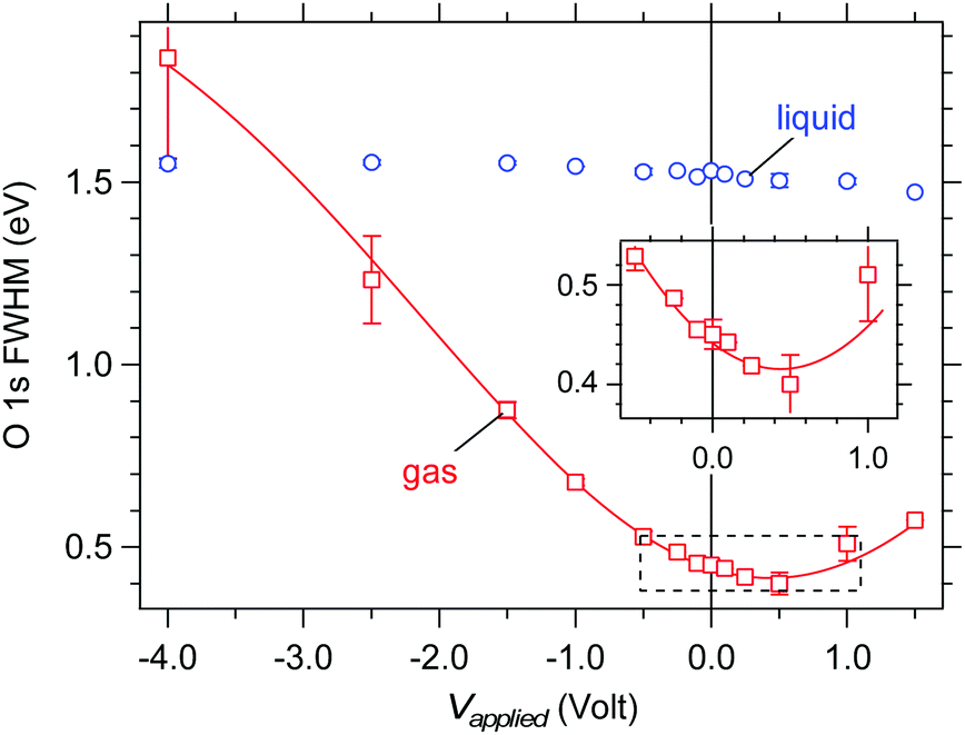
The full width at half the maximum (FWHM) of the O 1s gas phase component offers support to our finding of a vacuum level offset between the aqueous solution and the analyzer. Under an applied bias that exactly compensates the vacuum level offset the gas phase peak is expected to have its smallest FWHM as all gas molecules reside in an electric field-free region (see Fig. 7). The measured FWHM are shown in Fig. 10 as a function of applied bias. A minimum in the gas phase FWHM is observed at an applied bias of +0.5 V (red markers, see also the inset of Fig. 10), in qualitative agreement with the value of +0.60(±0.07) eV determined above for the vacuum level offset between the aqueous solution and the analyzer. We note that the fitting procedure is noticeably less reproducible under large applied bias (see error bars at −2.5 and −4.0 V bias in Fig. 10) because the peak becomes exceedingly broad and as such loses its appreciable intensity. However, the main focus of our discussion resides around small-applied bias where the fit and reproducibility are robust. The FWHM of the liquid component (Fig. 10, blue markers) shows no substantial effect with applied bias, broadening by a maximum 0.08 eV over the entire 5.5 V range, which confirms that the applied bias only acts to shift the energy levels of the aqueous solution relative to those of the analyzer but does not introduce any chemical change to the solution.

Fig. 10 Measured full width at half the maximum (FWHM) of the O 1s components as a function of applied bias on a liquid jet of 0.05 M NaCl. Blue: liquid O 1s component. Red: gas phase O 1s component. The solid line is a polynomial fit to the gas phase data and is intended only as a guide to the eye. The inset enlarges the region highlighted by the dashed box and shows a minimum in the FWHM of the gas component near +0.5 V applied bias.

Work functions of solid samples are determined in PES by measuring the secondary electron energy distribution curve (SEEDC) relative to the Fermi energy,²⁸ an approach that has been recently extended to aqueous solutions.²⁰ The work function is given by,

ϕ_water = hν − KE_Fermi + KE_cutoff + e·V_applied, (6)

where KE_Fermi is the kinetic energy of the Fermi level under no external bias, e is the elementary charge, and KE_cutoff is the kinetic energy cutoff of the SEEDC under an applied bias (V_applied). The Fermi energy of an aqueous solution is not evident in the spectra, which makes direct calculation of ϕ_water using eqn (6) non-trivial.²⁹ The SEEDC does, however, provide a direct measure of the difference between the vacuum levels of the aqueous solution and the analyzer,

(ϕ_water − ϕ_ana) = KE_cutoff + e·V_applied. (7)

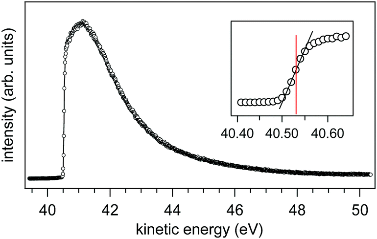
We have measured the SEEDC for 0.05 M NaCl at 273 K using a liquid jet of 22 μm (0.35 mL min⁻¹) under an applied bias of −40.00 V (Fig. 11). The onset energy is found at 40.53(±0.02) eV as determined from the inflection point of the rising edge (see inset of Fig. 11).³⁰ Using eqn (7) with KE_cutoff = 40.53 eV and V_applied = −40.00 V we find ϕ_water − ϕ_ana = +0.53(±0.02) eV.

Fig. 11 Secondary electron energy distribution curve (SEEDC) from a liquid jet of 0.05 M NaCl under an applied bias of −40.00 V. The inset shows the onset (40.53 eV) as determined from the inflection point of the rising edge.

Having established the vacuum level offset between 0.05 M NaCl and the analyzer using two different approaches (+0.60(±0.07) and +0.53(±0.02) eV) we are now in a position to report the first quantitative ionization energy from aqueous solution. Using eqn (2) with hν − KE = IE^meas_water = 537.64(±0.02) eV we find the real ionization energy of the O 1s orbital from liquid water in 0.05 M NaCl is 538.21(±0.07) eV. It is important to draw attention to the non-negligible correction applied to the measured O 1s ionization energy for this solution, (ϕ_water − ϕ_ana) = +0.57(±0.07) eV, as it highlights the scale by which previously reported measured ionization energies from aqueous solutions may be shifted from their real values.

Effect of solution composition on the vacuum level offset and ionization energy of an aqueous solution

In solid materials the vacuum level depends strongly on a plethora of internal and external factors that include purity, crystallographic orientation, morphology and surface composition, to name but a few.²⁸ Of particular interest for aqueous solutions are the cleanliness of the water–air (vacuum) interface and the chemical composition of the solution. The former becomes a non-issue when using the liquid jet—there is no spectroscopic evidence (see Fig. 4) to suggest even a partial layer of adventitious carbon contaminates the water–air (vacuum) interface as is traditionally observed with static aqueous solutions in vacuum.^20,31–34 In order to demonstrate the effect of solution composition on the vacuum level offset and ionization energy of an aqueous solution we have carried out an additional set of experiments for a solution of 0.15 M butylamine (CH₃–CH₂–CH₂–CH₂–NH₂, C 1s spectrum shown in Fig. 4) in 0.05 M NaCl. Butylamine is chosen because it partially segregates to the water–air interface and is therefore expected to have a large effect on the electron density and dipole orientation of the solution interface, but additionally because it contains no oxygen atom that might otherwise complicate the interpretation of the O 1s spectral region.

The response of this ternary solution to applied bias is determined in a manner analogous to that of 0.05 M NaCl using only a 19 μm nozzle and a flow rate of 0.30 mL min⁻¹ (Fig. 12). The liquid O 1s component shifts, as it did for the 0.05 M NaCl solution, in near-perfect agreement to the applied bias, the slope is 0.99(±0.01) eV V⁻¹ and the coefficient of determination from a linear regression fit to the data is R² = 0.999, while the gas phase slope is c = 0.70(±0.05) eV V^−1 35 with R² = 0.999. The measured ionization energies are 539.79(±0.02) eV (gas) and 537.74(±0.02) eV (liquid). Using eqn (5) with IE^real_gas = 539.82(±0.02) eV, IE^meas_gas = 539.79(±0.02) eV and c = 0.70(±0.05) eV V⁻¹ we determine that the vacuum level offset between the aqueous solution and the analyzer (ϕ_water − ϕ_ana) is +0.04(±0.04) eV. The FWHM of the gas phase O 1s component supports this finding, showing a pronounced minimum at 0 V bias (inset of Fig. 12). The real ionization energy is calculated with the minimal correction of +0.04(±0.04) eV (eqn (2)), and is 537.78(±0.04) eV for the liquid phase O 1s component.

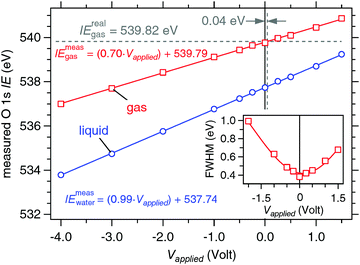Fig. 12 Response of the measured O 1s ionization energies to applied bias on a liquid jet of 0.15 M butylamine in 0.05 M NaCl. Blue: liquid O 1s component. Red: gas O 1s component. The solid lines are linear regression fits to the data sets. Measured ionization energies are calculated from eqn (1) (gas) and (3) (liquid). (inset) Measured full width at half the maximum (FWHM) of the O 1s gas component as a function of applied bias on a liquid jet of 0.15 M butylamine in 0.05 M NaCl. The solid line is a polynomial fit to the data and is intended only as a guide to the eye. The minimum in the FWHM is at 0.0 V bias.

It is common practice with PES measurements that employ (synchrotron) soft X-ray radiation in combination with a liquid jet to assume the IE of liquid water is independent of solution composition. Spectra from virtually any aqueous solution, irrespective of solute chemical composition or concentration [see for example ref. 7 (0.7 M cytidine in 1 M Tris–HF buffer), ref. 9 (1 M NaCl), ref. 16 (2 M imidazole), and ref. 36 (2 M guanidinium chloride in 2 M ammonium chloride)], are energy referenced to one of the published measured ionization energies of water taken in dilute (<0.05 M) electrolyte.^11,12 Our results, using the O 1s orbital of liquid water, reveal that the real ionization energy of liquid water depends on the chemical composition of the solution. Even in relatively dilute conditions compared to those of ref. 7, 9, 16 and 36 the addition of 0.15 M butylamine to a solution of 0.05 M NaCl results in a substantial shift in the O 1s ionization energy: −0.43 eV (the negative sign indicates the O 1s orbital moves closer to the vacuum level). In addition, the measured ionization energies of aqueous solutions published in the literature and used as energy reference are likely shifted from their real values by an undetermined vacuum level offset, which, in our case, is as much as +0.57 eV, but will certainly vary from instrument-to-instrument. A difference in work function between analyzers, which would not be surprising,²⁸ might offer a simple explanation for (at least part of) the discrepancy in the results of Winter et al. (11.16 eV)¹¹ and of Kurahashi et al. (11.31 eV)¹² for the IE of the 1b₁ orbital (HOMO) of liquid water. These seemingly small but significant details can no longer be ignored as PES from aqueous solutions transitions from the largely qualitative observations of the past decade towards the sort of quantitative (exact) results demanded by ever increasing levels of theory. For example, Gaiduk et al. recently calculated the valence band spectrum for an aqueous solution of 1 M NaCl using first principles.⁹ Eight different levels of theory were screened and their performance benchmarked by experiment. The accompanying PES measurement from a liquid jet of 1 M NaCl was, however, energy referenced to a solution of 0.03 M NaCl reported by Kurahashi et al.¹² By making this energy reference the authors implicitly imply (1) that the ionization energy of liquid water is independent of solution composition, and (2) that the measured ionization energies do not depend on the analyzer used. If we assume the experimental ionization energies reported in the study of Gaiduk et al. may be shifted from their real values by up to 0.57 eV (because the solution is 1 M NaCl and not 0.03 M, and the vacuum level offset was not quantified) then the level of theory deemed most successful would, in fact, be one of the least accurate.

The decrease in ionization energy of water upon the addition of butylamine can be rationalized by comparing the donor numbers of water and butylamine. Donor number is an experimental measure of the polarity of a (solvent) molecule, or its ability to act as an electron donor/acceptor.³⁷ In PES, donor number has been used to describe the relative ability of a molecule to screen the core-hole of a surrounding atom/molecule.³⁸ Molecules with higher donor numbers are more effective at screening the core-hole of a neighbouring ionized atom/molecule, which reduces the ionization energy. The donor number of butylamine (42 kcal mol⁻¹)³⁹ is more than two times greater than that of water (18 kcal mol⁻¹),³⁹ and therefore offers effectively two times better screening of the O 1s core-hole. This increased screening manifests itself as a shift to lower ionization energy.

The work function (electrochemical potential) of an aqueous solution

The results of our vacuum level offset measurements display an internal self-consistency that underscores its success. After all, our analysis using two different approaches for 0.05 M NaCl yield virtually the same result, with a mean (ϕ_water − ϕ_ana) = 0.57(±0.07) eV. The measured FWHM of the gas phase O 1s component when the vacuum levels of the aqueous solutions and analyzer are aligned are independent of the chemical composition of the solution, further credence to support its width depends directly on the vacuum level offset between the aqueous solutions and the analyzer (minima FWHM in Fig. 10 and 12 are equal). When the vacuum levels are equilibrated the gas behaves as if the liquid were not there and the natural line width of the gas is recovered. The vacuum level offset together with knowledge of the work function of the analyzer (ϕ_ana = 4.08(±0.06) eV, see Experimental methods), enables quantitative determination of the work function, or more commonly, the electrochemical potential of the aqueous solution. We find values of ϕ_water = 4.65(±0.09) eV for 0.05 M NaCl, and ϕ_water = 4.12(±0.07) eV for 0.15 M butylamine in 0.05 M NaCl. Similar to the behaviour of a solid surface²⁸ we find the work function of water depends strongly on the chemical composition at the interface. It is non-trivial to compare the present quantitative results for a dilute aqueous solution of 0.05 M NaCl, 4.65(±0.09) eV, to that estimated previously for a saturated solution of NaCl (∼6 M), ϕ_water = 5.0(±0.5) eV, as the saturated solution interface contained an abundance of several different carbon contaminants.²⁰ The effect of this carbon-contamination was not systematically evaluated in ref. 20 and so the work function of a clean saturated solution of NaCl is not known.

The 0.05 eV width of the rising edge of the SEEDC (inset of Fig. 11) is at least an order of magnitude more narrow than those previously reported for aqueous solutions, 0.5 eV²⁰ and 0.7 eV,⁴⁰ and allows the onset energy to be determined simply by the inflection point of the rising edge.^30,41 We attribute the narrow width of the rising edge primarily to the cleanliness of the liquid microjet—no adventitious carbon contamination to introduce heterogeneity, new dipoles or a redistribution of electron density at the air–water interface, but additionally, at least in the case of the UV study of Faubel from 1997,⁴⁰ to the higher resolution of modern analyzers. This result ensures that the level of accuracy attainable for quantitative measure of the vacuum level offset (and subsequently the work function of an aqueous solution) is no worse than those for solids.

Conclusions

In summary, this report presents a systematic approach to determine quantitative ionization energies for aqueous solutions using liquid jet X-ray photoelectron spectroscopy. Exact core (or valence) level ionization energies are determined only after accounting for the vacuum level offset between the aqueous solution and the photoelectron analyzer. We presented two different methods for quantifying this offset, which display a self-consistency that underscores its success. Accounting for the vacuum level offset in the calculation of ionization energies revealed that the O 1s ionization energy of liquid water is not, as is traditionally assumed in the literature, independent of the chemical composition of the solution. The observed shift to lower ionization energy upon addition of 0.15 M butylamine to an aqueous solution of 0.05 M NaCl is explained by the higher donor number of butylamine compared with water, and thereby its ability to more effectively screen the core-hole of a neighbouring ionized water molecule.

The work function, or electrochemical potential of the aqueous solution is derived from the vacuum level offset between the aqueous solution and the photoelectron analyzer. Similar to the well-known behaviour of solid surfaces in vacuum, the work function was shown to vary with the chemical composition of the interface. By adding 0.15 M butylamine to an aqueous solution of 0.05 M NaCl the work function was reduced by 0.53 eV. We suspect this effect is caused by a redistribution of the water–air (vacuum) surface dipole but further investigation, accompanied by the appropriate theoretical support, is needed to validate this hypothesis. This work is on going in our laboratory.

Acknowledgements

A portion of this work was performed at the SIM beamline of the Swiss Light Source (SLS), Paul Scherrer Institute, Villigen, Switzerland. G. O. acknowledges funding from an ETH Research Grant (no. ETH-20 13-2). A. G. and M. A. B. acknowledge funding from the Swiss National Science Foundation (no. 153578). D. C. acknowledges funding from the Slovenian Research Agency (P1-0112).

Notes and references

1. D. Grand, A. Bernas and E. Amouyal, Chem. Phys., 1979, 44, 73–79.
2. N. S. Kim and P. R. LeBreton, J. Am. Chem. Soc., 1996, 118, 3694–3707.
3. H. Fernando, G. A. Papadantonakis, N. S. Kim and P. R. LeBreton, Proc. Natl. Acad. Sci. U. S. A., 1998, 95, 5550–5555.
4. C. E. Crespo-Hernandez, R. Arce, Y. Ishikawa, L. Gorb, J. Leszczynski and D. M. Close, J. Phys. Chem. A, 2004, 108, 6373–6377.
5. P. Slavicek, B. Winter, M. Faubel, S. E. Bradforth and P. Jungwirth, J. Am. Chem. Soc., 2009, 131, 6460–6467.
6. E. Cauet, M. Valiev and J. H. Weare, J. Phys. Chem. B, 2010, 114, 5886–5894.
7. C. A. Schroeder, E. Pluharova, R. Seidel, W. P. Schroeder, M. Faubel, P. Slavicek, B. Winter, P. Jungwirth and S. E. Bradforth, J. Am. Chem. Soc., 2015, 137, 201–209.
8. R. Seidel, B. Winter and S. E. Bradforth, Annu. Rev. Phys. Chem., 2016, 67, 283–305.
9. A. P. Gaiduk, M. Govoni, R. Seidel, J. H. Skone, B. Winter and G. Galli, J. Am. Chem. Soc., 2016, 138, 6912–6915.
10. R. G. Pearson, J. Am. Chem. Soc., 1986, 108, 6109–6114.
11. B. Winter, R. Weber, W. Widdra, M. Dittmar, M. Faubel and I. V. Hertel, J. Phys. Chem. A, 2004, 108, 2625–2632.
12. N. Kurahashi, S. Karashima, Y. Tang, T. Horio, B. Abulimiti, Y. I. Suzuki, Y. Ogi, M. Oura and T. Suzuki, J. Chem. Phys., 2014, 140, 174506.
13. K. R. Siefermann, Y. X. Liu, E. Lugovoy, O. Link, M. Faubel, U. Buck, B. Winter and B. Abel, Nat. Chem., 2010, 2, 274–279.
14. A. T. Shreve, T. A. Yen and D. M. Neumark, Chem. Phys. Lett., 2010, 493, 216–219.
15. B. Jagoda-Cwiklik, P. Slavicek, L. Cwiklik, D. Nolting, B. Winter and P. Jungwirth, J. Phys. Chem. A, 2008, 112, 3499–3505.
16. P. R. Tentscher, R. Seidel, B. Winter, J. J. Guerard and J. S. Arey, J. Phys. Chem. B, 2015, 119, 238–256.
17. N. Kharche, J. T. Muckerman and M. S. Hybertsen, Phys. Rev. Lett., 2014, 113, 176802.
18. W. L. Jolly, K. D. Bomben and C. J. Eyermann, At. Data Nucl. Data Tables, 1984, 31, 433–493.
19. R. Sankari, M. Ehara, H. Nakatsuji, Y. Senba, K. Hosokawa, H. Yoshida, A. De Fanis, Y. Tamenori, S. Aksela and K. Ueda, Chem. Phys. Lett., 2003, 380, 647–653.
20. H. Tissot, J. J. Gallet, F. Bournel, G. Olivieri, M. G. Silly, F. Sirotti, A. Boucly and F. Rochet, Top. Catal., 2016, 59, 605–620.
21. M. A. Brown, M. Faubel and B. Winter, Annu. Rep. Prog. Chem., Sect. C: Phys. Chem., 2009, 105, 174–212.
22. M. A. Brown, A. Beloqui Redondo, I. Jordan, N. Duyckaerts, M.-T. Lee, M. Ammann, F. Nolting, A. Kleibert, J. P. Machler, M. Birrer, H. J. Wörner and J. A. van Bokhoven, Rev. Sci. Instrum., 2013, 84, 073904.
23. G. Olivieri, A. Goel, A. Kleibert and M. A. Brown, J. Synchrotron Radiat., 2015, 22, 1528–1530.
24. N. Preissler, F. Buchner, T. Schultz and A. Lubcke, J. Phys. Chem. B, 2013, 117, 2422–2428.
25. M. A. Brown, Z. Abbas, A. Kleibert, A. Goel, S. May and T. M. Squires, Phys. Rev. X, 2016, 6, 011007.
26. A. Chaudhuri, T. J. Lerotholi, D. C. Jackson, D. P. Woodruff and V. Dhanak, Phys. Rev. Lett., 2009, 102, 126101.
27. S. Axnanda, M. Scheele, E. Crumlin, B. H. Mao, R. Chang, S. Rani, M. Faiz, S. D. Wang, A. P. Alivisatos and Z. Liu, Nano Lett., 2013, 13, 6176–6182.
28. A. Kahn, Mater. Horiz., 2016, 3, 7–10.
29. The Fermi energy can be indirectly determined from an equivalent measurement of SEEDC on a conductive solid sample in a parallel experiment or in a separate experiment under otherwise identical photon energy and applied bias conditions using, for instance, a gold wire mounted in the position of the liquid jet. This procedure was employed in ref. 20 albeit using an extended polycrystalline gold foil.
30. G. Ertl and J. Küppers, Low Energy Electrons and Surface Chemistry, VCH Verlagsgesellschaft, Weinheim, Germany, 1985.
31. M. H. Cheng, K. M. Callahan, A. M. Margarella, D. J. Tobias, J. C. Hemminger, H. Bluhm and M. J. Krisch, J. Phys. Chem. C, 2012, 116, 4545–4555.
32. S. Ghosal, M. A. Brown, H. Bluhm, M. J. Krisch, M. Salmeron, P. Jungwirth and J. C. Hemminger, J. Phys. Chem. A, 2008, 112, 12378–12384.
33. S. Ghosal, J. C. Hemminger, H. Bluhm, B. S. Mun, E. L. D. Hebenstreit, G. Ketteler, D. F. Ogletree, F. G. Requejo and M. Salmeron, Science, 2005, 307, 563–566.
34. M. J. Krisch, R. D'Auria, M. A. Brown, D. J. Tobias, J. C. Hemminger, M. Ammann, D. E. Starr and H. Bluhm, J. Phys. Chem. C, 2007, 111, 13497–13509.
35. The geometric correction factor, c, is specific to the geometry of the experiment and is therefore expected to be, within the reproducibility of the measurements, the same for each sample investigated. Our results are consistent with this interpretation of c.
36. J. Werner, E. Wernersson, V. Ekholm, N. Ottosson, G. Ohrwall, J. Heyda, I. Persson, J. Soderstrom, P. Jungwirth and O. Bjorneholm, J. Phys. Chem. B, 2014, 118, 7119–7127.
37. C. Reichardt, Solvents and Solvent Effects in Organic Chemistry, Wiley-VCH GmbH and Co., 3rd edn, 2003.
38. M. El Kazzi, I. Czekaj, E. J. Berg, P. Novak and M. A. Brown, Top. Catal., 2016, 59, 628–634.
39. F. Cataldo, Eur. Chem. Bull., 2015, 4, 92–97.
40. M. Faubel, B. Steiner and J. P. Toennies, J. Chem. Phys., 1997, 106, 9013–9031.
41. This procedure is very accurate for solid samples because of the sharp rising edge of the SEEDC. In previous SEEDC measurements from aqueous solutions, see e.g., ref. 20 and 40, the rising edges are broad, 0.5 and 0.7 eV, respectively, and such a straightforward determination of the cutoff energy is non-trivial. In ref. 20 it was concluded that the determination of the SEEDC energy cutoff in liquids appears somewhat arbitrary because of this broad rising edge. In an attempt to circumvent the ambiguity of determining the cutoff energy an exponentially modified Gaussian function was used to fit the SEEDC in ref. 20 and 40. Our rising edge is more than an order of magnitude more narrow (0.05 eV) and as such we have implemented the well accepted approach employed to determine the energy cutoff in solid samples (as shown in ref. 30).

---