The role of a small-scale cutoff in determining molecular layers at fluid interfaces

Abstract

The existence of molecular layers at liquid/vapour interfaces has been a long debated issue. More than ten years ago it was shown, using computer simulations, that correlations at the liquid/vapour interface resemble those of bulk liquids, even though they can be detected in experiments only in a few cases, where they are so strong that they cannot be concealed by the geometrical smearing of capillary fluctuations. The results of the intrinsic analysis techniques used in computer experiments, however, are still often questioned because of their dependence on a free parameter that usually represents a small-scale cutoff used to determine the interface. In this work I show that there is only one value of the cutoff that can ensure a quantitative explanation of the intrinsic density correlation peaks in terms of successive layer contributions. The value of the cutoff coincides, with a high accuracy, with the molecular diameter.

---

1 Introduction

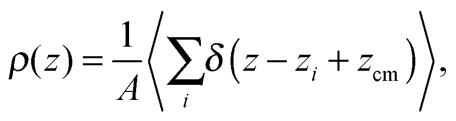
The presence of a definite microscopic structure at the interface between two fluids, similar to that at a liquid/solid interface,¹ has always been debated. Since the very first theoretical and numerical investigations^2,3 it has emerged that even simple liquids might display a pronounced layered structure at the liquid/vapour interface. These observations were not backed up by experiments, and soon thereafter it was concluded from simulation studies on larger systems that oscillations in the density profile were artefacts of insufficient sampling.⁴

Later on it became clear that the presence of surface fluctuations induces a smearing of the density profiles, leading to the commonly observed sigmoidal shapes. The density profile, deconvoluted from the surface waves, is usually referred to as the intrinsic density profile.⁵ In a way, the intrinsic density profile is not conceptually different from a usual density profile. The latter, even though it is often not mentioned explicitly, expresses the correlation, along the macroscopic normal to the interface, z, between a particle's position and that of the centre of mass of the system,

where 〈⋯〉 denotes a canonical average, A is the simulation box cross-sectional area, z_i is the coordinate of the i-th particle, and z_cm is the coordinate of the centre of mass of the system. Without correlating the particle's position with the centre of mass, one would obtain simply the one-particle density, a constant, as in a proper canonical sampling the centre of mass of the system would span the whole available space. If the correlation is performed instead with respect to the local position of the interface ξ(x_i,y_i), one obtains the intrinsic profileFor some liquids the correlations at the surface are so strong that some traces of them “survive” the smearing of capillary waves⁶ and can be observed in the non-intrinsic density profile and also detected, for example, by X-ray reflectivity measurements. This is the case for the liquid metals Ga⁷ and Hg.⁸ It turns out that it is reasonable to expect some kind of layering in every simple or molecular liquids, at least far from the critical temperature.⁹ The assumption of a layered structure of the intrinsic density profile of the kindhas proven to fit well the intrinsic profile of simple liquids, and has been used to show that deviations from capillary wave theory due to correlation effects are restricted to the first few layers.⁹

In this sense, there is probably no doubt left that the intermolecular correlations present in the bulk show up also at the interface, and that the oscillations of the intrinsic density profile can be related to the presence of successive layers.¹⁰ However, one should keep in mind that in order to calculate the intrinsic profile, a continuous surface should be identified, and this has to be derived from the (discrete) set of atoms. As such, the surface is just an ancillary construct, not a well-defined physical object, and suffers, in all of its many operative definitions, from some ambiguity. These are usually represented by some kind of small-scale cutoff used to define the surface itself, be it the distance used in the intrinsic sampling method of Chacón and Tarazona,⁹ the grid size in the method of Jorge and Cordeiro,¹¹ the Gaussian width in Willard and Chandler's method¹² or the probe sphere radius of the Identification of Truly Interfacial Molecules (ITIM) approach.¹³ In a critical comparison of several methods,^14,15 the optimal value of the cutoff parameter was sought, for example, by requiring the distribution in the first layer to differ the least from a Gaussian. The dependence of the intrinsic profile on the value of the cutoff parameter was also instead investigated, for example, for the grid-based method^11,16 and for the intrinsic sampling method.¹⁷

A common denominator of these results is that for values of the cutoff parameter close to the molecular size, the Gaussian shape of the distribution of atoms in the first layer is preserved, and the overall shape of the intrinsic profile (at least at distances not too close to the interface) is remarkably robust, that is, the profiles are not very sensitive to the choice of the cutoff value itself. Here I show that the separate contributions of successive layers to the intrinsic profile are, instead, much more sensitive to the cutoff value. At first glance a disadvantage, this feature becomes the key to showing that the value of the cutoff is precisely the molecular diameter or, vice-versa, that only using the molecular diameter as a natural cutoff, the intrinsic profile correlations can be explained in terms of successive molecular layers.

2 Methods, results and discussion

Simulations of liquid argon (2237 atoms arranged in a slab configuration in a box of 4 × 4 × 18 nm³) in the canonical ensemble were performed using the Nosé–Hoover thermostat^18,19 (with a relaxation time of 0.1 ps) at temperature T = 85 K, namely, close to the triple point. Argon molecules have been modelled using the Lennard-Jones potential U(r) = 4ε[(σ/r)¹² − (σ/r)⁶], known to reproduce well its liquid structure,²⁰ with the Rahman parameters²¹ε = 120 K and σ = 0.34 nm, where σ represents an effective molecular diameter. Periodic boundary conditions have been imposed in all three directions, and the dispersion part of the pair interactions has been computed by taking care of the periodic copies using the smooth Particle Mesh Ewald method²² for the Lennard-Jones interaction with a Gaussian width of 0.246 nm, and a mesh size of 0.15 nm. The equations of motion have been integrated using a leapfrog algorithm with a timestep of 1 fs for 500 ps of equilibration followed by 1 ns of sampling. The velocity of the center of mass has been subtracted every 100 steps, and the configurations of the system have been saved to disk for later analysis with the same frequency.

The simulations as described above have been performed using the molecular dynamics simulation package GROMACS version 5.1,²³ while the analysis of the intrinsic profiles has been performed using the (planar) ITIM algorithm¹³ as implemented in ref. 24. The algorithm works as follows: for every stored configuration, the molecules in the liquid phase have been selected, by a simple cluster analysis with a cutoff of 0.5 nm, as those belonging to the largest cluster. Conversely, all molecules not belonging to the largest cluster (mostly monomers) are considered to belong to the vapour phase.²⁵ Surface molecules are then identified as those which come first in contact with probe spheres of diameter d moving from the gas phase to the liquid one. A probe sphere and an argon molecule are considered to be in contact when their distance is equal to (d + σ)/2. Once the molecules in the first layer have been selected, the ITIM procedure is repeated to identify the second layer, and so on, up to the fifth one.

The resulting intrinsic density profiles, calculated for different values of the probe sphere radius, are reported in Fig. 1, together with the pair correlation function, normalized to match the bulk density. The probe sphere diameter d ranges from 0.2 to 0.4 nm, namely, from about 60 to 120% of the Lennard-Jones parameter σ. All intrinsic density profiles share the same qualitative features, with maxima located at, or in close proximity of, the corresponding peak of the radial distribution function. One distinctive trend is that the density close to the surface becomes larger upon increasing the probe sphere radius. This can be easily understood if one considers the limiting behaviour for an infinitely large probe sphere radius, where only one atom (the outermost) would be identified as a surface one, contributing to the delta peak at z − ξ = 0, while all other atoms, no matter how small their distance from the interface z − ξ, would contribute to the remaining part of the density profile.

Fig. 1 Intrinsic density profiles of the liquid/gas interface of Ar in the liquid region, for different values of the probe sphere diameter, ranging from 0.4 nm (curve that penetrates most in proximity to the origin) to 0.2 nm (curve with the largest depletion close to the origin). The pair correlation function, rescaled to fit the bulk number density, is also reported and identifiable by the more pronounced oscillations.

As it was anticipated in the Introduction, the density profile turns out to be a rather robust feature. For example, to the 60% rescaling of the probe sphere diameter d mentioned above (that is, a change from 0.34 to 0.20 nm), the position of the second peak (z − ξ ≃ −0.35 nm) moves only by 6%, and its height by 12%. For the third peak, the corresponding figures are even smaller. The robustness of the total intrinsic profile is related to the fact that as soon as the long-wave fluctuations at the surface are filtered out (which are also those with the largest amplitudes), the underlying intrinsic profile starts emerging, as the main source of smearing is removed.

This picture changes dramatically if one looks at the contributions to the intrinsic profile coming from different layers, reported in Fig. 2, for the sake of clarity, for a selected set of probe sphere diameters d = 0.20, 0.32, 0.34, 0.36, and 0.40 nm.

Fig. 2 Intrinsic density profiles of the liquid/gas interface of Ar in the liquid region, for different values of the probe sphere diameter (from the top to the bottom, d = 0.40 to 0.20 nm, respectively) together with the contributions of the second, third, fourth and, fifth layers.

In this case, the corresponding distributions of the layer contributions (the middle panel and the lowest panel) are not even comparable. If the probe sphere diameter d is chosen to have the same value as the molecular one d = σ = 0.34 nm, the layer profiles become clearly peaked at the corresponding maxima of the intrinsic profile, and show an unimodal distribution. In contrast, in the d = 0.20 nm, as well as in the d = 0.40 nm cases, the peaks of the layers are shifted with respect to the corresponding intrinsic profile maxima, and show the clear presence of shoulders. For the two remaining cases (d = 0.32 and d = 36 nm), it is still possible to see, especially in the third and fourth peak, respectively, that the layer distribution is not exactly peaked at the corresponding maxima of the intrinsic profile.

This sensitivity to the probe-sphere size emerges because the fact of belonging to a specific coordination layer, rather than to another one, is determined by correlations at the scale of the molecular size, as opposed to the smearing of capillary waves, which occurs predominantly at long wavelengths.

In order to perform a more quantitative analysis of these shifts, it is possible to determine the peak location by performing a Gaussian fit in the proximity of the maxima both for the total intrinsic profile and for the layer contributions. The result of this fit is shown in Fig. 3, where the peak position is reported as a function of the probe sphere diameter d for the first four peaks after the surface one (which is always a delta function at z − ξ = 0). In the second peak case, the peak position itself does not depend, by any practical means, on the probe sphere diameter, and the values coming from the best fits to the total profile and to the first layer contribution almost always coincide.

Fig. 3 Position of the different peaks in the total intrinsic profile (circles) and in the different layers (squares), as a function of the probe sphere diameter d. Lines are guides to the eye that connect neighboring points.

The third, fourth and fifth peaks show a much more interesting behaviour. The positions of the peaks, determined from the fit to the total intrinsic profile, are also in this case only weakly dependent on the probe sphere diameter, confirming once more that the total intrinsic profile has rather stable features. In contrast, the peak positions determined from the fit to the successive layers show a much stronger dependence on d, and are located deeper towards the bulk for smaller probe sphere radii, and closer to the interface for larger ones. As expected from the qualitative trend shown already in Fig. 2, the two lines clearly cross at the value d = σ.

A closer inspection of the [0.32, 0.36] nm region shows that the two curves cross at a values d = σ within 0.01 nm. This is a rather strong indication that the structure of the peaks close to the interfaces can be interpreted in terms of a self-consistent definition of successive layers, only if the probe-sphere diameter is chosen to be the same as the molecular diameter, σ.

One question is left open, namely, whether it is possible to find a similar criterion for non-spherical molecules. In the present case, the Lennard-Jones diameter is a reasonable estimate of the smallest accessible distances between molecules. This is not the case, for example, for water, where instead the first peak of the radial distribution function is located at a distance smaller than the Lennard-Jones diameter, because of the presence of strong electrostatic forces. In this case, one would expect the optimal probe sphere diameter to be smaller than the Lennard-Jones one, although this point needs further investigation.

3 Conclusions

In this work, an analysis of the properties of successive molecular layers, as a function of the small-scale cutoff used to identify them, has been presented. Contrary to the total intrinsic profile, which was found to be rather insensitive to small changes of the cutoff, the distributions of the molecular layers below the interfacial one turned out to depend more markedly on it. The reason for the robustness of the total intrinsic profile is that the intrinsic structure starts emerging as soon as the long-wave fluctuations of the interface are removed, no matter what is the fine grain detail of the filtering procedure. In contrast, it is the position correlations at the molecular scale that determine to which layer the molecules belong. In order to match these two scales and reconcile the picture of the intrinsic profile peaks with that of successive molecular layers, one has to use a well-defined value of the small-scale cutoff (here, the ITIM probe sphere size), which turns out to be, within 0.01 nm, the molecular size itself, σ.

It should be stressed here that, so far, no a priori prescription exists, on what the criterion for choosing a small-scale cutoff should be and, in this sense, that choice ultimately reflects our ideas on what characterizes a “proper” surface. The added value of the present approach, however, is that it introduces self-consistency to the description of the layering at the interface and this, hopefully, will help dispel the doubts about the significance of molecular layers at liquid/liquid and liquid/vapour interfaces.

References

1. F. F. Abraham, J. Chem. Phys., 1978, 68, 3713–3716.
2. C. A. Croxton and R. P. Ferrier, J. Phys. C: Solid State Phys., 1971, 4, 1909.
3. J. W. Perram and L. R. White, Faraday Discuss. Chem. Soc., 1975, 59, 29–37.
4. G. A. Chapela, G. Saville and J. S. Rowlinson, Faraday Discuss. Chem. Soc., 1975, 59, 22–28.
5. J. S. Rowlinson and B. Widom, Molecular Theory of Capillarity, Oxford University Press, Oxford, 1982.
6. E. Chacón, M. Reinaldo-Falagán, E. Velasco and P. Tarazona, Phys. Rev. Lett., 2001, 87, 166101.
7. M. J. Regan, E. H. Kawamoto, S. Lee, P. S. Pershan, N. Maskil, M. Deutsch, O. M. Magnussen, B. M. Ocko and L. E. Berman, Phys. Rev. Lett., 1995, 75, 2498–2501.
8. O. M. Magnussen, B. M. Ocko, M. J. Regan, K. Penanen, P. S. Pershan and M. Deutsch, Phys. Rev. Lett., 1995, 74, 4444–4447.
9. E. Chacón and P. Tarazona, Phys. Rev. Lett., 2003, 91, 166103.
10. M. Sega, B. Fábián and P. Jedlovszky, J. Chem. Phys., 2015, 143, 114709.
11. M. Jorge and M. N. D. S. Cordeiro, J. Phys. Chem. C, 2007, 111, 17612.
12. A. P. Willard and D. Chandler, J. Phys. Chem. B, 2010, 114, 1954–1958.
13. L. B. Pártay, G. Hantal, P. Jedlovszky, Á. Vincze and G. Horvai, J. Comput. Chem., 2008, 29, 945–956.
14. M. Jorge, P. Jedlovszky and M. N. D. S. Cordeiro, J. Phys. Chem. B, 2010, 114, 11169–11179.
15. M. Jorge, P. Jedlovszky and M. N. D. S. Cordeiro, J. Phys. Chem. B, 2010, 114, 18656–18663.
16. M. Jorge and M. N. D. S. Cordeiro, J. Phys. Chem. C, 2007, 111, 17612–17626.
17. E. Chacón and P. Tarazona, J. Phys.: Condens. Matter, 2005, 17, S3493.
18. S. Nosé, Mol. Phys., 1984, 52, 255–268.
19. W. G. Hoover, Phys. Rev. A: At., Mol., Opt. Phys., 1985, 31, 1695–1697.
20. J. L. Yarnell, M. J. Katz, R. G. Wenzel and S. H. Koenig, Phys. Rev. A: At., Mol., Opt. Phys., 1973, 7, 2130–2144.
21. A. Rahman, Phys. Rev., 1964, 136, A405.
22. U. Essman, L. Perera, M. L. Berkowitz, T. Darden, H. Lee and L. G. Pedersen, J. Chem. Phys., 1995, 103, 8577–8593.
23. S. Páll, M. Abraham, C. Kutzner, B. Hess and E. Lindahl, in Solving Software Challenges for Exascale, ed. S. Markidis and E. Laure, Springer International Publishing, 2015, vol. 8759.
24. M. Sega, S. S. Kantorovich, P. Jedlovszky and M. Jorge, J. Chem. Phys., 2013, 138, 44110.
25. B. Senger, P. Schaaf, D. S. Corti, R. Bowles, J.-C. Voegel and H. Reiss, J. Chem. Phys., 1999, 110, 6421.

---

References

- F. F. Abraham, J. Chem. Phys., 1978, 68, 3713–3716 CrossRef CAS