
 Open Access Article
 This Open Access Article is licensed under a
 Creative Commons Attribution 3.0 Unported Licence
Modeling blue to UV upconversion in β-NaYF4:Tm3+†
Pedro
Villanueva-Delgado
 *a,
Karl W.
Krämer
a,
Rafael
Valiente
b,
Mathijs
de Jong
c and
Andries
Meijerink
c
*a,
Karl W.
Krämer
a,
Rafael
Valiente
b,
Mathijs
de Jong
c and
Andries
Meijerink
c
aDepartment of Chemistry and Biochemistry, University of Bern, 3012 Bern, Switzerland. E-mail: pedro.villanueva@dcb.unibe.ch
bDepartamento de Física Aplicada, Facultad de Ciencias, Universidad de Cantabria-IDIVAL, 39005 Santander, Spain
cCondensed Matter and Interfaces, Debye Institute for Nanomaterials Science, Utrecht University, 3508TA Utrecht, The Netherlands
First published on 2nd September 2016
Abstract
Samples of 0.01% and 0.3% Tm3+-doped β-NaYF4 show upconverted UV luminescence at 27![[thin space (1/6-em)]](https://www.rsc.org/images/entities/char_2009.gif) 660 cm−1 (361 nm) after blue excitation at 21140 cm−1 (473 nm). Contradictory upconversion mechanisms in the literature are reviewed and two of them are investigated in detail. Their agreement with emission and two-color excitation experiments is examined and compared. Decay curves are analyzed using the Inokuti–Hirayama model, an average rate equation model, and a microscopic rate equation model that includes the correct extent of energy transfer. Energy migration is found to be negligible in these samples, and hence the average rate equation model fails to correctly describe the decay curves. The microscopic rate equation model accurately fits the experimental data and reveals the strength and multipolarity of various interactions. This microscopic model is able to determine the most likely upconversion mechanism.
660 cm−1 (361 nm) after blue excitation at 21140 cm−1 (473 nm). Contradictory upconversion mechanisms in the literature are reviewed and two of them are investigated in detail. Their agreement with emission and two-color excitation experiments is examined and compared. Decay curves are analyzed using the Inokuti–Hirayama model, an average rate equation model, and a microscopic rate equation model that includes the correct extent of energy transfer. Energy migration is found to be negligible in these samples, and hence the average rate equation model fails to correctly describe the decay curves. The microscopic rate equation model accurately fits the experimental data and reveals the strength and multipolarity of various interactions. This microscopic model is able to determine the most likely upconversion mechanism.
1 Introduction
Upconversion (UC) is the absorption of two or more low-energy photons and the subsequent emission of a high-energy photon.1 Several trivalent lanthanide ions are commonly used for this purpose, for example singly doped or codoped into insulator lattices. Tm3+ ions can emit light at different wavelengths from the NIR to the UV and show upconversion in singly doped samples under NIR, red, and blue excitation.2–5 Tm3+ codoped with Yb3+ also shows particularly strong blue and UV emission under 980 nm excitation.6–8There are different applications of upconversion phosphors, for example in biomedical research,9 dental medicine,10 photovoltaic energy production,11 and photocatalysis.12,13
The detailed mechanism of singly doped Tm3+ upconversion under different excitation energies has been studied in several crystalline and vitreous environments. However, the actual processes involved are not clear for the case of blue excitation that results in UV emission.2 These processes may also be responsible for the efficient blue and UV emission in samples codoped with Yb3+.7
There are several energy transfer (ET) processes that lead to upconversion. In this work we will examine two of them: energy transfer upconversion (ETU) and cross-relaxation (CR). Both processes have the same requirements: two ions in close proximity and resonance between energy states (spectral overlap).
Two kinds of ET interactions are possible, multipolar or exchange, depending on the distance between the ions and the electronic orbital overlap.14 For the β-NaYF4:Tm3+ samples investigated in this paper, the exchange interaction is not significant as the minimum distance between rare earth ions in β-NaYF4 is 3.53 Å and the low doping increases the average first neighbor distance to more than 10 Å.15,16 In the multipolar case, the strength of the interaction W can be expanded as a series of inverse powers of the distance R between the sensitizer (S) and the activator (A):17
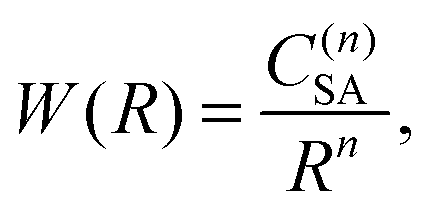 | (1) |
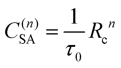
where n is the multipolarity of the interaction, n = 6, 8, and 10 for dipole–dipole (d–d), dipole–quadrupole (d–q), and quadrupole–quadrupole (q–q), respectively, and C(n)SA is a constant that depends on the multipolarity. The dominant multipolarity of a transition depends on the symmetry of the states involved.14,18
Several models have been developed to predict the decay of a sensitizer in the presence of an activator under different assumptions. The Inokuti–Hirayama model, for example, predicts the decay curve of a sensitizer that can decay radiatively or transfer its energy to an activator situated nearby. Other interactions such as energy migration among the sensitizers or ET to excited states of the activator (ETU or CR) are not taken into account.19 The random lattice positions of the activator and the combination of the two relaxation pathways produce a non-exponential decay, especially at the beginning of the decay curve. The beginning of the curve is mostly affected by the ET to the activator, while the tail of the curve reproduces the single exponential decay of the sensitizer. The analytical form is given by
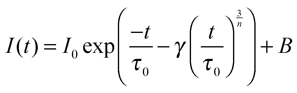 | (2) |
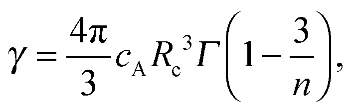 | (3) |
 | (4) |
A recent microscopic rate equation model includes the effect of the crystalline environment (the distances between the ions) and the finite speed of energy migration.16 This model can predict the dynamics of a system at different dopant concentrations and excitation powers. A fit to experimental data provides the most likely critical radius and multipolarity of the different interactions.
2 Experimental methods
Microcrystalline powder samples of β-NaYF4:0.3% Tm3+ and β-NaYF4:0.01% Tm3+ were synthesized as described in ref. 29.Visible and NIR emission spectra and decay curves were recorded using an Opotek Opolette HE 355II laser as an excitation source with a pulse width of 7 ns and a repetition rate of 10 Hz. An Edinburgh Instruments FLS920 spectrophotometer with a 0.3 m single emission monochromator and Hamamatsu R928 UV/VIS or R5509-73 NIR photomultiplier tubes (PMTs) were used to detect the light. An Edinburgh Instruments PCS900 single-photon counter and multichannel analyzer were used to record the decay curves.
The two-color pump and probe excitation experiments were carried out using an Opotek Opolette HE 355II (7 ns pulse) and an Ekspla NT342B-10-SH/DUV OPO (5 ns pulse) as excitation sources (both with 10 Hz repetition rate), a 0.55 m TRIAX 550 single emission monochromator, and a Hamamatsu R928 PMT. The signal was analyzed using a Stanford Research SR400 gated photon counter. Both laser pulses were synchronized using a Standford Research DG535 pulse generator to arrive at the sample at the same time. The UV upconversion emission spectra were recorded using the same setup but using only the Ekspla laser as an excitation source.
All measurements were performed at room temperature.
3 Results
The powder X-ray diffractograms of the β-NaYF4:0.01% Tm3+ and β-NaYF4:0.3% Tm3+ samples correspond to the pure hexagonal β-NaREF 4 phase (RE = rare earth ion) that crystallizes in the space group P![[6 with combining macron]](https://www.rsc.org/images/entities/char_0036_0304.gif) . The RE3+ sites with C1 and C3h symmetry have both a nine-fold coordination by F− ions and are randomly occupied by Y3+ and Tm3+ ions,15 see Fig. S1, ESI.†
. The RE3+ sites with C1 and C3h symmetry have both a nine-fold coordination by F− ions and are randomly occupied by Y3+ and Tm3+ ions,15 see Fig. S1, ESI.†
Fig. 1 shows the emission spectra of β-NaYF4 doped with 0.3% and 0.01% Tm3+ after 3H6 → 1G4 excitation at 21140 cm−1 (473 nm). Both samples have been investigated under the same experimental conditions. The peaks have been assigned to f–f transitions of Tm3+ based on their lifetimes and energies, according to the Dieke diagram.30
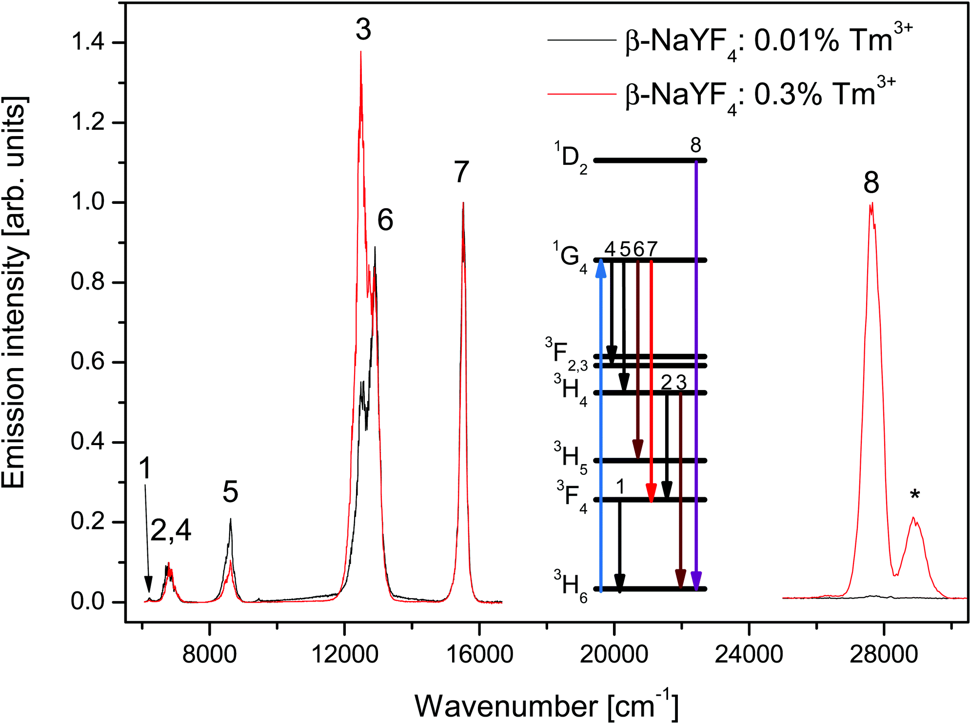 | ||
| Fig. 1 Emission spectra of β-NaYF4 doped with 0.3% Tm3+ (red line) and 0.01% Tm3+ (black line) after 3H6 → 1G4 excitation at 21140 cm−1. The low energy side is normalized to the 1G4 → 3F4 emission intensity. The high energy side (1D2 → 3H6) was recorded using a different detector, but otherwise with the same settings for both samples. The band marked with an asterisk (*) corresponds to the Tm3+ 3P0 → 3F4 emission. | ||
The low energy side of the spectra shows emission from the 1G4, 3H4, and 3F4 states to the 3H6 ground state and other intermediate states. The spectra are normalized to the 1G4 → 3F4 emission intensity. The major differences observed between the two samples are the 3H4 → 3H6 and 1G4 → 3H4 emission intensities. The former emission is about 2.5 times stronger in the 0.3% sample than in the 0.01% sample, the latter however is 2 times weaker. These differences are discussed in Section 4.
The small peak close to 6200 cm−1 (numbered 1 in Fig. 1) is assigned to the 3F4 → 3H6 transition. Since the detector efficiency strongly decreases towards that end of the spectrum, that peak's position and intensity can only be taken as indicative.
The band centered at 6780 cm−1 (numbered 2 and 4 in Fig. 1) is assigned to the transitions 3H4 → 3F4 and 1G4 → 3F3. The different peaks in the band have decay curves that correspond to the 3H4 or 1G4 states, see Fig. 2b and c. Most of the band intensity originates from the 3H4 → 3F4 transition, see Fig. 3a, and also Fig. S2, ESI.†
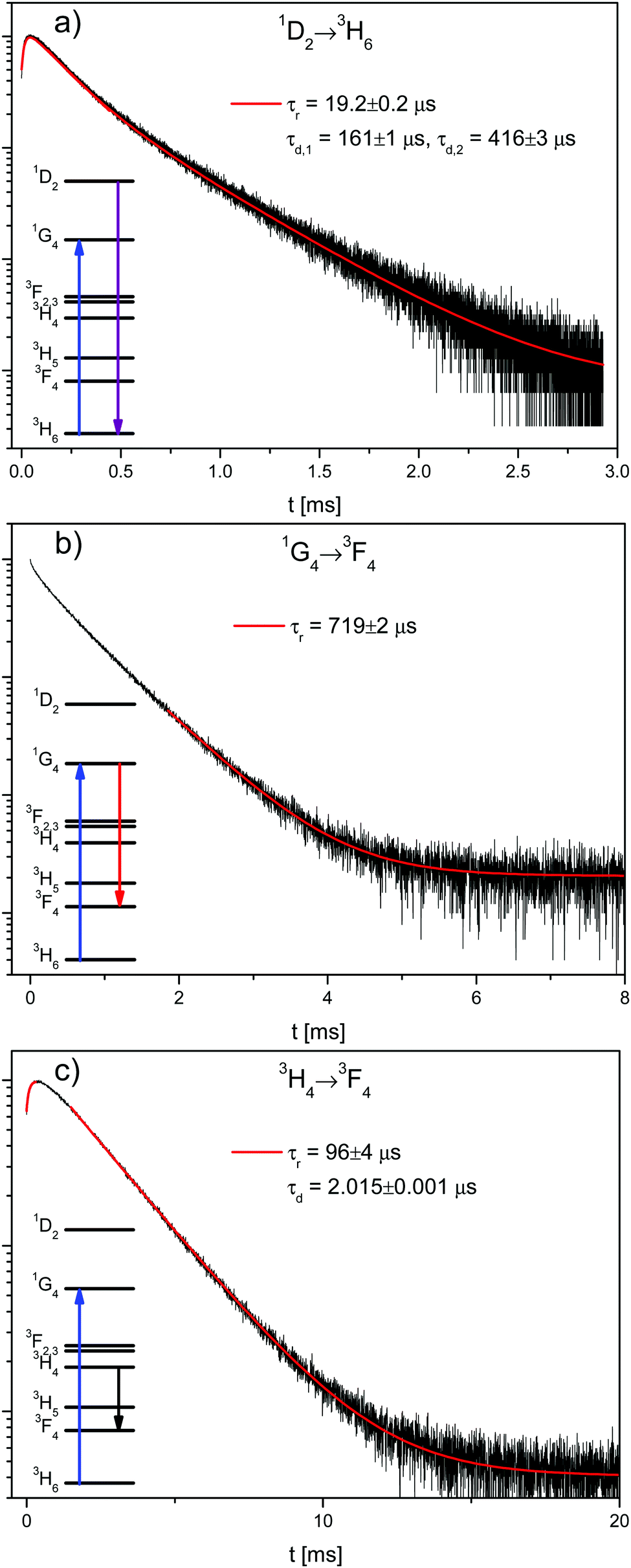 | ||
| Fig. 2 Decay curves of β-NaYF4:0.3% Tm3+ (black lines) after 3H6 → 1G4 excitation (at 21140 cm−1) with exponential rise τr and decay τd fits (red lines). (a) 1D2 → 3H6 transition with a single exponential fit to the rise and a double exponential fit to the decay. (b) 1G4 → 3F4 transition with a single exponential fit to the decay. (c) 3H4 → 3F4 transition with single exponential rise and decay fits. | ||
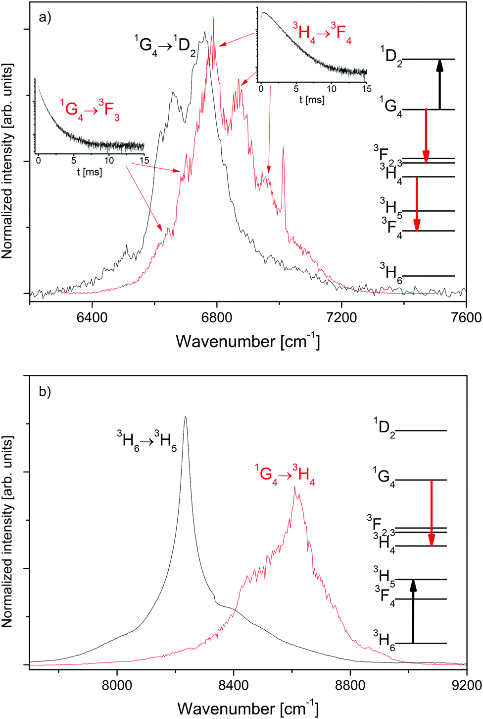 | ||
| Fig. 3 Spectral overlap (normalized to the area) of selected transitions in β-NaYF4:0.3% Tm3+. (a) 1G4 → 1D2 excited state absorption (black line) and 3H4 → 3F4/1G4 → 3F3 emissions (red line). (b) 3H6 → 3H5 ground state absorption (black line) and 1G4 → 3H4 emission (red line). The respective transitions are indicated in the Tm3+ energy state diagrams on the right hand side. | ||
The high energy side of the spectra was recorded using a different detector and the intensities cannot be compared with the low energy side. The emission intensity of the 0.01% sample is 50 times weaker than that of the 0.3% sample. Aside from the 1D2 → 3H6 emission, a peak corresponding to the 3P0 → 3F4 emission is present in the spectra. The mechanism responsible for the population of the 3P0 state is beyond the scope of this paper. An ETU process from the 1D2 or 1G4 states is likely, as an ESA process from the 1G4 state is not resonant with any Tm3+ state.
Fig. 2 shows the decay curves of the 1D2 → 3H6, 1G4 → 3F4, and 3H4 → 3F4 transitions in β-NaYF4:0.3% Tm3+. The reason that the 1G4 → 3H6 decay is not shown here is due to the difficulty of measuring its emission close to the excitation energy. The 3H4 → 3F4 decay has been chosen instead of the 3H4 → 3H6 because the latter is very close in energy to the 1G4 → 3H5 emission and its rise time is partially masked by it. All decay curves from the 1G4 and 3H4 states are shown in Fig. S4, ESI.†
The 1G4 → 3F4 decay in Fig. 2b is not single exponential, which is evidence of energy transfer. The tail decay time is τd = 719 μs, which is shorter than the intrinsic lifetime τ = 758 μs, see Fig. S3b, ESI.† The most salient feature in Fig. 2a and c is the fast rise time of τr = 19 μs and τr = 96 μs, respectively. The decay of the 1D2 → 3H6 transition is not single exponential with fast and slow decay components of τd,1 = 161 μs and τd,2 = 416 μs, respectively. Both decay times are slower than the intrinsic 1D2 lifetime of τ = 67.5 μs, see Fig. S3a, ESI.† The 3H4 → 3F4 decay lifetime of τd = 2.015 ms is very similar to the 3H4 → 3H6 decay lifetime of 1.94 ms observed for the direct excitation of the 3H4 state in the 0.01% sample at low power, see Fig. S3c, ESI.†
The spectral overlap of selected transitions in β-NaYF4:0.3% Tm3+ is presented in Fig. 3. Fig. 3a shows the spectral overlap between the 1G4 → 1D2 excited state absorption, see Fig. S5, ESI,† and the 3H4 → 3F4 and 1G4 → 3F3 emission bands, see Fig. 1. The strong overlap between the transitions is a necessary condition for the ETU processes 3H4 + 1G4 → 3F4 + 1D2 and 1G4 + 1G4 → 3F3 + 1D2 between two interacting Tm3+ ions in close proximity.
Fig. 3b compares the ground state absorption 3H6 → 3H5, see Fig. S6, ESI,† to the 1G4 → 3H4 emission, see Fig. 1. The overlap is smaller than that in Fig. 3a, but still significant. Thus the CR process 3H6 + 1G4 → 3H5 + 3H4 is a possible ET process between two nearby Tm3+ ions.
4 Analysis
In the literature, contradictory Tm3+ upconversion mechanisms are proposed for the population of the 1D2 state after 1G4 excitation. Often, one ETU step processes are proposed: 1G4 + 1G4 → 3F3 + 1D2,33F3 + 3F3 → 3H6 + 1D2,6,7 or 1G4 + 1G4 → 3H4 + 1D2.2 Those investigations were carried out in different host lattices (including glasses). Samples additionally codoped with Yb3+ are sometimes used, which complicates the analysis. The different crystal-field environments result in small shifts in energy that may affect the resonance between transitions and thus different mechanisms may be responsible for the 1D2 upconversion in different samples. A recent work has studied the role of CR steps in depopulating the 1D2, 1G4, and 3H4 states for downconversion.31We now consider two upconversion mechanisms: schemes I and II, shown in Fig. 4. Scheme I involves two ET processes and three Tm3+ ions. Scheme II involves an ETU process, multiphonon relaxation, and two Tm3+ ions. Both schemes explain the very fast rise times of the 1D2 and 3H4 states, see Fig. 2a and c.
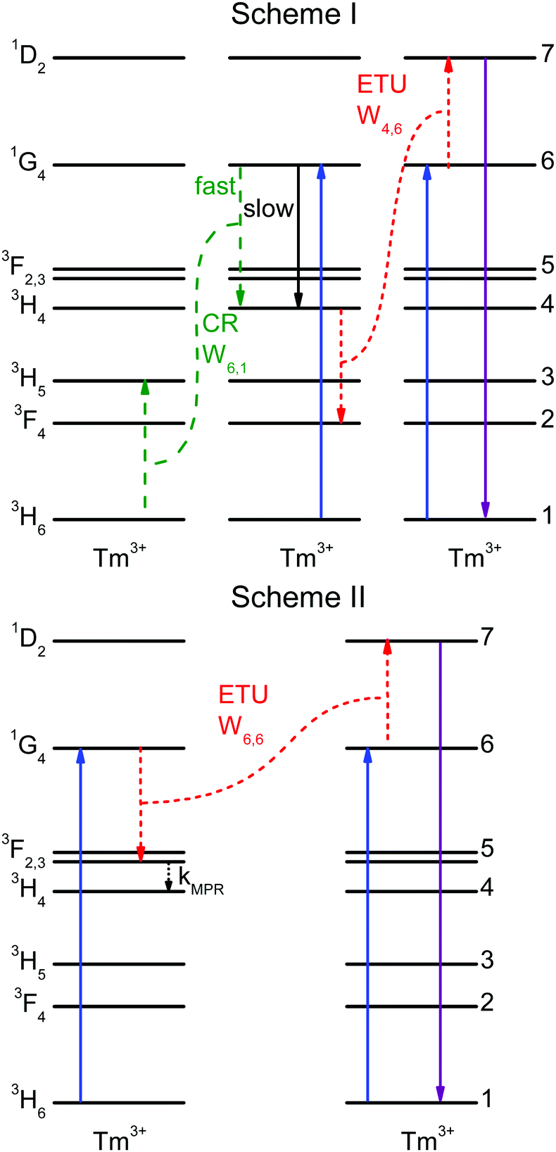 | ||
| Fig. 4 Possible mechanisms for 1D2 upconversion in Tm3+. The blue arrow 3H6 → 1G4 indicates the excitation and the violet arrow shows the 1D2 → 3H6 upconverted UV emission. The Wi,j denote ET processes with initial states i and j. Scheme I: two ET processes populate the 3H4 and 1D2 states. The 1G4 → 3H4 radiative transition (black arrow, slow) and the CR step (green arrows, fast) populate the 3H4 state. The ETU step (red) populates the 1D2 state. Scheme II: one ETU process populates the 1D2 state. Rapid multiphonon relaxation (MPR) from 3F3 populates the 3H4 state. | ||
Scheme I: the 1G4 → 3H4 decay time of 719 μs is much slower than the 96 μs rise time of the 3H4 luminescence, see Fig. 2b and c. Accordingly, the 3H4 state cannot be directly populated by the 1G4 state. But energy transfer processes between two ions can affect a state population very quickly; in fact, the CR step 3H6 + 1G4 → 3H5 + 3H4 is able to populate the 3H4 state very rapidly. The emission spectra, see Fig. 1, support this statement. The spectra of both samples are very similar except for the 3H4 → 3H6 and 1G4 → 3H4 transitions. The 3H4 → 3H6 transition is stronger (by a factor of 2.5) in the 0.3% Tm3+ sample as a result of the CR process that populates the 3H4 state. This process depends on the Tm3+ concentration and hence it is stronger for the 0.3% Tm3+ sample. The 1G4 → 3H4 transition, however, is weaker (by a factor of 2) in the 0.3% Tm3+ sample while other transitions from the 1G4 state are not. It is possible that radiative energy transfer 1G4 + 3H6 → 3H4 + 3H5 plays a role in the higher doped sample, whereby a Tm3+ ion in the ground state absorbs a photon emitted from the 1G4 → 3H4 decay in another Tm3+ ion. Unfortunately, it is not possible to reliably measure the 3H5 → 3H6 and 3F4 → 3H6 emissions (see below).
Scheme II: the ETU process 1G4 + 1G4 → 3F3 + 1D2 can populate the 1D2 state rapidly and fast multiphonon relaxation from 3F3 to 3H4 can explain the fast rise time of the 3H4 state. The different emission intensities of the 3H4 → 3H6 and 1G4 → 3H4 transitions are explained in the same way as in scheme I.
The width of the emission bands in this lattice made it impossible to measure the decay curve of the 3H5 → 3H6 transition, as it is masked by the 1G4 → 3H4 emission; the 3F4 → 3H6 emission is at the edge of the detector sensitivity and therefore cannot be measured reliably. The 3H5 → 3H6 decay curve could offer valuable information to decide which of the two schemes prevails.
In order to discover which mechanism explains the experimental data better, we proceed to analyze the data in view of three models: the Inokuti–Hirayama model, an average rate equation model, and a microscopic rate equation model that takes the correct extent of energy transfer into account.
4.1 The Inokuti–Hirayama
The samples of β-NaYF4:Tm3+ contain only one optically active ion. In this case the sensitizer in the Inokuti–Hirayama model corresponds to the Tm3+ ions excited in the 1G4 state, while the activator are those ions in the ground state.The 1G4 → 3F4 decay has been fitted to the Inokuti–Hirayama model according to eqn (2), for the three different interaction multipolarities n = 6 (d–d), n = 8 (d–q), and n = 10 (q–q), see Fig. 5 and Table S1, ESI.† All fits are in good agreement with the experimental data, the best being that for dipole–dipole interaction. It is possible that all multipolarities play a role in the energy transfer process.
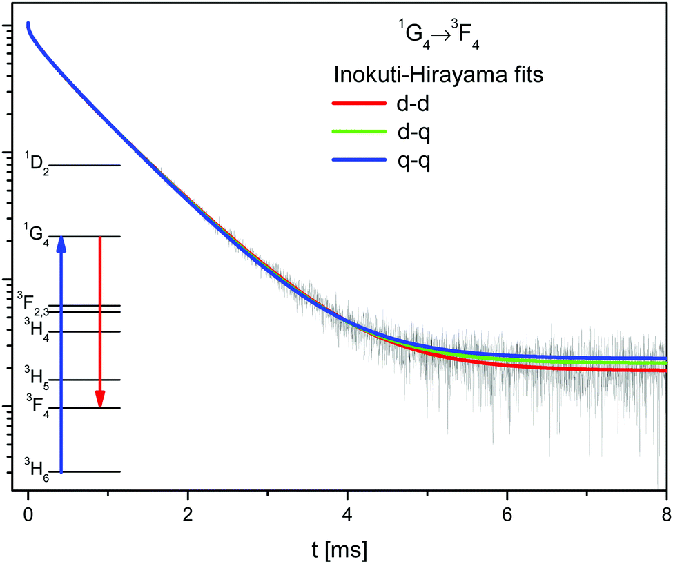 | ||
| Fig. 5 Decay of the 1G4 state (black line) in β-NaYF4:0.3% Tm3+ with the Inokuti–Hirayama fit for dipole–dipole (d–d), dipole–quadrupole (d–q), and quadrupole–quadrupole (q–q) interaction mechanisms. | ||
In order to determine the interaction critical radius using eqn (3), the activator concentration cA has to be obtained. cA is the concentration of Tm3+ ions in the ground state, and is related to the fraction FE of excited Tm3+ ions in the 1G4 state right after the excitation pulse: cA = (1 − FE)cTm3+, where cTm3+ is the concentration of Tm3+ ions in the sample, cTm3+ = 4.14 × 10¹⁹ ions cm−3 for β-NaYF4:0.3% Tm3+. FE can be estimated from the absorption transition probability RP and the pulse duration Δt. The absorption probability is given by
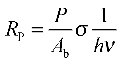 | (5) |
The absorption cross-section for 3H6 → 1G4 is σ = 7.77 × 10⁻²² cm2, see Fig. S6, ESI.† For the laser used in these experiments the relevant parameters are P = 6 × 10⁶ W, Ab = 3 × 10⁻² cm2, and Δt = 5 ns, which results in RP = 3.67 × 10⁵ s−1 and FE ≈ RPΔt ≈ 0.2%. Therefore, most Tm3+ ions remain in the ground state after the pulse and cA ≈ cTm3+.
Using the values determined above and eqn (3), the critical radius for the d–d CR process is Rc,IH = 11.8 ± 0.1 Å. This value is similar to those found in other lattices for other Tm3+ interactions.31,35,36
The Inokuti–Hirayama model agrees well with the experimental data due to the low concentration of Tm3+ ions. The long distances between Tm3+ ions restrict the extent of energy migration. The 1G4 decay has also been fitted using the Burshtein, Zusman and Yokota–Tanimoto models, see Fig. S7, ESI.† These models introduce energy migration among the sensitizers in addition to the sensitizer–activator ET. For all these models the fit results in zero or negligible energy migration rates.
The decay curve is therefore affected only by the energy transfer to nearby Tm3+ ions and the intrinsic radiative decay of the 1G4 state. Although the Inokuti–Hirayama model correctly predicts the 1G4 decay curve and shows that energy migration is absent, it does not make any predictions about the 3H4 and 1D2 decay curves or the specific ET processes (ETU and/or CR) that take place. A rate equation model can give information about the decay curves of all states and the ET processes involved.
4.2 Average rate equation model
The excitation, emission, CR, and ETU processes can be modeled with the help of a rate equation system.26,37 This is a system of n differential equations that depend on n variables (the energy state populations) and the time t. In this case n = 7, as the states higher in energy than 1D2 do not participate in the mechanism, see Fig. 4. The population of state i (i = 1,…,7) is denoted by yi, e.g. the population of the ground state is y1.The absorption and emission processes shown in Fig. 1 and the energy transfer processes depicted in Fig. 4 are expressed mathematically in eqn (6). The absorption of light corresponding to the 3H6 → 1G4 transition is modeled with RP(y1 − 13/9y6), where RP is the absorption probability, see eqn (5). The first term in the parentheses refers to stimulated absorption and the second to stimulated emission (13/9 is the relative degeneracy of the initial and final states). The decay is modeled with a decay rate constant ki that includes the radiative and non-radiative contributions. The emission from state i to state f is modeled with a branching ratio parameter βi,f. For example, for the 3H5 state the term β6,3k6y6 (with β6,3 < 1) indicates that a fraction of the decay from state 6 (1G4) populates state 3 (3H5). Energy transfer steps with initial states i and j are modeled with Wi,jyiyj, where Wi,j is a constant to be fitted using experimental data. Eqn (6) shows the state populations in red to help distinguish the linear and non-linear terms.
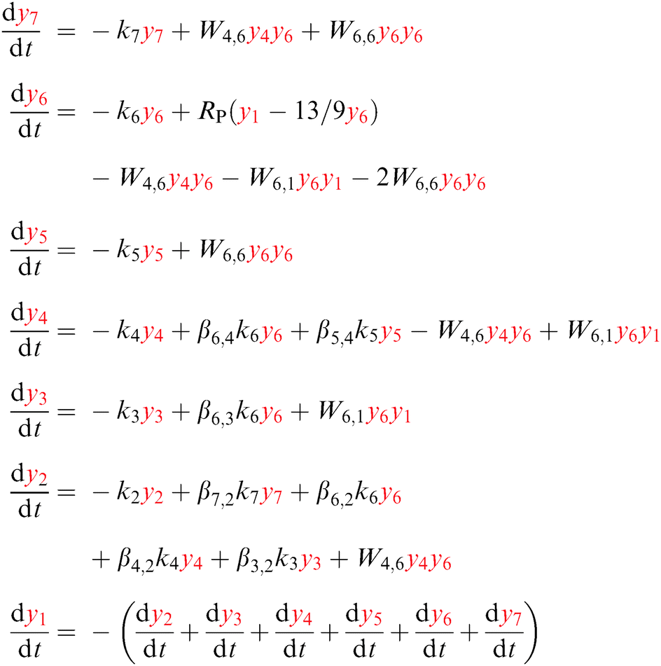 | (6) |
The 3F3 state decays mainly to the 3H4 state, so the decay rate k5 is the multiphonon relaxation rate kMPR shown in Fig. 4.
The solution to the system of equations is the population of each state as a function of time. The free parameters are the CR rate W6,1 and the ETU rate W4,6 (with W6,6 = 0) for scheme I and the ETU rate W6,6 (with W6,1 = W4,6 = 0) and the decay rate k5 for scheme II. The parameters for both schemes were fitted to the experimental data and are shown as dashed lines in Fig. 6. The best fit values of the parameters for scheme I are W6,1 = 2.13 × 10³ s−1 (CR rate) and W4,6 = 1.10 × 10⁸ s−1 (ETU rate), whereas they are W6,6 = 1.58 × 10⁷ s−1 and kMPR = 1.00 × 10⁶ s−1 for scheme II.
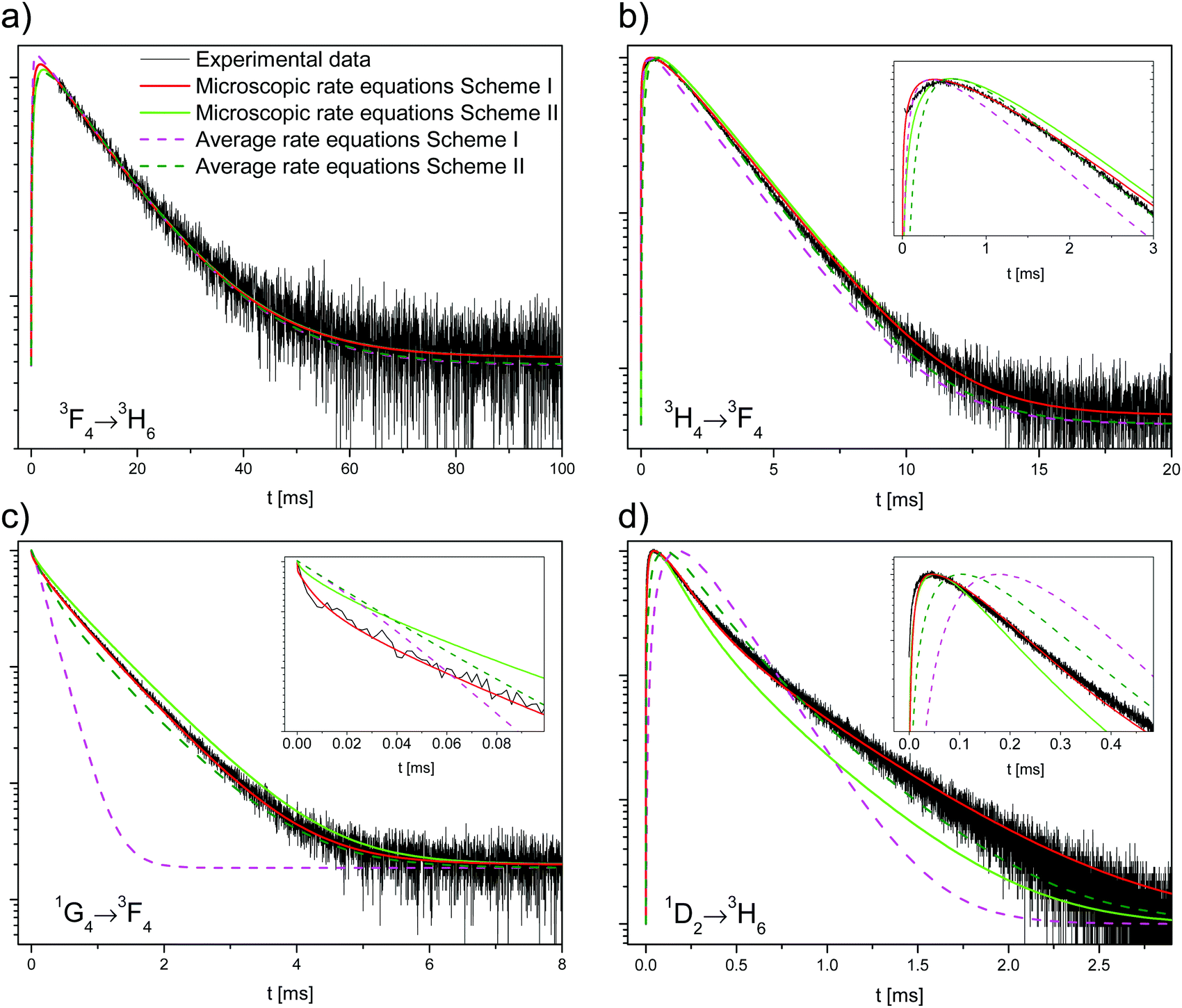 | ||
| Fig. 6 Experimental data and calculated decay curves. (a) 3F4, (b) 3H4, (c) 1G4, and (d) 1D2 state decays. The experimental data are plotted as black lines, the fits to the average rate equation model as dashed lines (scheme I, magenta; scheme II, olive), and the fits to the microscopic rate equation model as full lines (scheme I, red; scheme II, green). The insets show the decay at the short time scale. | ||
Neither fit to the average rate equation model is able to correctly reproduce the decay of the 1G4 and 1D2 states, especially for scheme I. The reason for this strong discrepancy with the experimental data is the absence of energy migration in the samples. There are two classes of excited ions: isolated ions that decay radiatively to the ground state and those that transfer their energy to another ion. Most ions belong to the former group, and hence the measured lifetime of the 1G4 decay (719 μs) is very similar to the intrinsic single exponential decay (760 μs). Ions in the latter group have a much faster decay rate as they efficiently transfer their energy.
The average rate equation model assumes infinitely fast energy migration among all ions in the sample so that the population of each state does not deviate much from the average.26,28 For these samples however, as previously demonstrated, energy migration is negligible. A more sophisticated microscopic rate equation model that can predict the decay curves of all states and correctly takes into account the correct extent of energy transfer is presented in the next subsection.
4.3 Microscopic rate equation model
A β-NaYF4:0.3% Tm3+ lattice with 50 × 50 × 50 unit cells is simulated and the distances between all ions are calculated, up to dmax = 150 Å. Then a rate equation system like eqn (6) is assigned to each Tm3+ ion in the lattice. For a concentration of 0.3% this results in 571 Tm3+ ions in the simulation. The ET rates are calculated taking into account the distances to the other ions and the chosen multipolarity of the interaction with eqn (1). These Wi,j rates are not average ET parameters but actually the CSA rates in eqn (1). The resulting nonlinear system of differential equations has 3997 variables, corresponding to 7 energy states for 571 ions. Its solution is the population of each state as a function of time. In order to compare the model with the experimental data, the average of each state is calculated across all ions.16 A fit of the parameters to the experimental data is performed. The fit normalized root-mean-square deviation εtotal is calculated by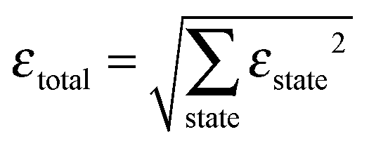 | (7) |
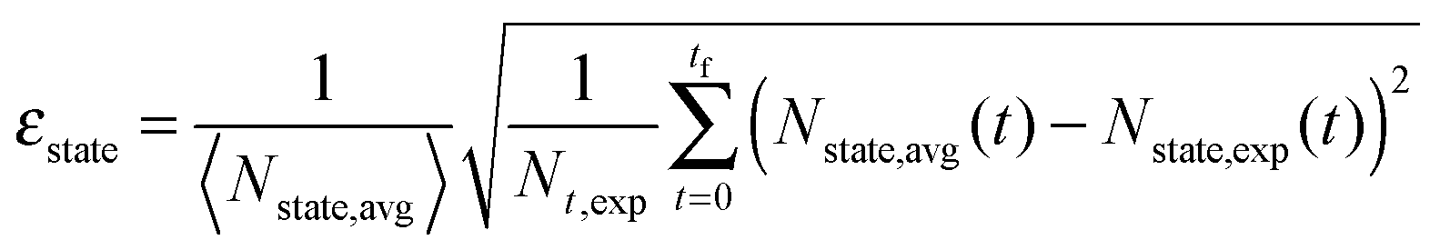 | (8) |
The values of the fixed parameters are given in Table 2 and the values of the lifetimes and branching ratios are the same as for the average rate equation model given in Table 1.
| Fixed parameter | Value |
|---|---|
| a | 5.9734(6) Å |
| c | 3.5296(4) Å |
| N cells | 125000 |
| d max | 150 Å |
| c Tm (0.3 mol%) | 4.14 × 10¹⁹ ions cm−3 |
|
σ (ν = 21100 cm−1) |
7.77 × 10⁻²² cm2 |
|
1.7 × 10⁷ W cm−2 |
| Δtpulse | 5 ns |
The results of the simulation are compared to the experimental data in Fig. 6. Scheme I (red lines) fits the experimental data better than scheme II (green lines), with a normalized root-mean-square deviation of εI = 0.49 versus εII = 0.68.
For scheme I, the fitted values are W4,6 = 1.258 × 10−38 cm6 s−1 (d–d interaction) for the ETU and W6,1 = 4.205 × 10−39 cm6 s−1 (d–d interaction) for the CR. The corresponding critical radii are Rc,ETU = 16.9 Å and Rc,CR = 12.1 Å. The agreement between experiment and simulation is excellent. The simulation correctly reproduces all decay curves, especially the rise of the 3H4 and 1D2 states, the non-exponential decay of the 1D2 state, and the shape of the 1G4 curve at the short timescale. For both ET steps, the dipole–dipole interaction (n = 6) gives the best fit to the experimental data, see Table S2, ESI.†
The critical radius of Rc,CR = 12.1 Å for the CR process is very similar to Rc,IH = 11.8 ± 0.1 Å for the Inokuti–Hirayama fit. This can be understood since the CR process is a transfer to an ion in its ground state, precisely the only kind of ET process that the Inokuti–Hirayama model deals with. The population of the 1D2 state is small and the effect of the ETU on the 1G4 decay curve is negligible, so the simple Inokuti–Hirayama fit is not much affected by it. However, both ET processes contribute to the decay curve of the 3H4 state.
For scheme II, the best fit for the ETU rate is W6,6 = 1.60 × 10⁻³⁵ cm6 s−1 with multipolarity n = 6 (d–d) and 3F3 decay rate kMPR = 3.26 × 10⁸ s−1. The corresponding critical radius is Rc,ETU = 47.9 Å, a value that is much larger than the usual range of 5–20 Å.31,35,36 Fischer et al. have estimated the energy gap law parameters for this lattice.37 Using a conservative estimate of the energy difference between the 3H4 and 3F3 states of ΔE = 1800 cm−1 the estimated rate is kMPR = 4.61 × 10⁴ s−1, several orders of magnitude smaller than the fitted value of 3.26 × 10⁸ s−1. The magnitudes of the optimized parameters for scheme II are physically unreasonable. Together with the higher fit error, it is concluded that scheme II cannot explain the experimental data correctly.
For either scheme, including energy migration among the Tm3+ ions does not improve the fit, in agreement with the results in Section 4.1.
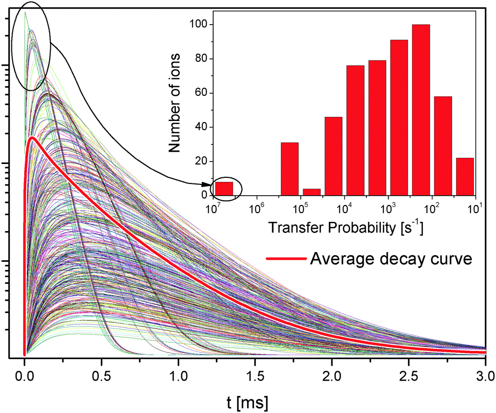 | ||
| Fig. 7 All 1D2 simulated decay curves of the 571 Tm3+ ions in a β-NaYF4:0.3% Tm3+ sample of 50 × 50 × 50 unit cells. The average population is shown as a thick red curve. The inset shows the histogram of the number of ions with a given energy transfer probability to its nearest neighbor. The ions with a higher transfer probability have faster rise and decay times. | ||
The transfer probability depends on the inverse sixth power of the distance, see eqn (1); this means that small differences in the distance have a large effect on the transfer probability, see the inset in Fig. 7.
Fig. 7 shows all 1D2 state decay curves from the 571 Tm3+ ions in the simulated lattice introduced above. The average decay curve is shown as a thick red line and is the same as in Fig. 6d.
Some ions reach the 1D2 state much faster than others and with a much higher probability. Those ions have neighbors at the nearest possible distance, and therefore interact very strongly; their decay curves dominate the average decay curve at the short timescale. Some other ions have neighbors further away and become excited at later times; they dominate the average decay curve at longer times. Because of the discrete nature of the distances in the lattice, the ET probability between two ions drops from about 6 × 10⁶ s−1 to 3 × 10⁵ s−1 for separations of 3.53 Å and 5.9 Å, respectively.
The features in the decay curves of other states have similar microscopic origins; however, since the 1D2 population requires two ET steps, this state is more strongly affected than others by the lattice distance distribution.
5 Conclusions
Two Tm3+–Tm3+ energy transfer processes are responsible for the upconverted UV luminescence in β-NaYF4:Tm3+ after 3H6 → 1G4 blue excitation at 21140 cm−1: the cross-relaxation step 3H6 + 1G4 → 3H5 + 3H4 and the energy transfer upconversion step 3H4 + 1G4 → 3F4 + 1D2. The alternative mechanism consisting of the energy transfer upconversion step 1G4 + 1G4 → 3F3 + 1D2 and non-radiative relaxation 3F3 → 3H4 cannot explain all experimental data. It requires unreasonable parameters for the upconversion and multiphonon relaxation rates.
The interaction strength and multipolarity have been determined for each process from a fit to experimental data. All results indicate that energy migration is negligible in these samples and that all energy transfer processes are due to dipole–dipole interactions.
The microscopic rate equation model accurately fits the experimental data and offers a detailed view on the ion to ion energy transfer processes. This microscopic model is a significant improvement on other models such as Inokuti–Hirayama and the average rate equation models because it takes into account the distances between ions and all decay and energy transfer processes in the sample, including energy migration.
Acknowledgements
The financial support of the EU FP7 ITN LUMINET (Grant agreement No. 316906) is gratefully acknowledged.References
- F. Auzel, Chem. Rev., 2004, 104, 139–174 CrossRef CAS PubMed.
- A. Gharavi and G. L. McPherson, Chem. Phys. Lett., 1992, 200, 279–282 CrossRef CAS.
- H. Yang and J. Gao, Phys. B, 2013, 426, 31–34 CrossRef CAS.
- E. Cantelar, G. Torchia and F. Cussó, J. Lumin., 2007, 122–123, 459–462 CrossRef CAS.
- G. Özen, A. Kermaoui, J. Denis, X. Wu, F. Pelle and B. Blanzat, J. Lumin., 1995, 63, 85–96 CrossRef.
- R. J. Thrash and L. F. Johnson, J. Opt. Soc. Am. B, 1994, 11, 881–885 CrossRef CAS.
- M. A. Noginov, M. Curley, P. Venkateswarlu, A. Williams and H. P. Jenssen, J. Opt. Soc. Am. B, 1997, 14, 2126–2136 CrossRef CAS.
- X. X. Zhang, P. Hong, M. Bass and B. H. T. Chai, Phys. Rev. B: Condens. Matter Mater. Phys., 1995, 51, 9298–9301 CrossRef CAS.
- J. Zhou, Q. Liu, W. Feng, Y. Sun and F. Li, Chem. Rev., 2015, 115, 395–465 CrossRef CAS PubMed.
- A. Stepuk, D. Mohn, R. N. Grass, M. Zehnder, K. W. Krämer, F. Pellé, A. Ferrier and W. J. Stark, Dent. Mater., 2012, 28, 304–311 CrossRef CAS PubMed.
- J. C. Goldschmidt and S. Fischer, Adv. Opt. Mater., 2015, 3, 510–535 CrossRef CAS.
- W. Yang, X. Li, D. Chi, H. Zhang and X. Liu, Nanotechnology, 2014, 25, 482001 CrossRef PubMed.
- Y. Chen, S. Mishra, G. Ledoux, E. Jeanneau, M. Daniel, J. Zhang and S. Daniele, Chem. – Asian J., 2014, 9, 2415–2421 CrossRef CAS PubMed.
- O. Malta, J. Non-Cryst. Solids, 2008, 354, 4770–4776 CrossRef CAS.
- A. Aebischer, M. Hostettler, J. Hauser, K. Krämer, T. Weber, H. U. Güdel and H.-B. Bürgi, Angew. Chem., Int. Ed., 2006, 45, 2802–2806 CrossRef CAS PubMed.
- P. Villanueva-Delgado, K. W. Krämer and R. Valiente, J. Phys. Chem. C, 2015, 119, 23648–23657 CAS.
- M. Quintanilla, E. Cantelar, F. Cussó, J. A. Barreda-Argüeso, J. González, R. Valiente and F. Rodríguez, Opt. Mater. Express, 2015, 5, 1168–1182 CrossRef.
- T. Kushida, J. Phys. Soc. Jpn., 1973, 34, 1318–1326 CrossRef CAS.
- M. Inokuti and F. Hirayama, J. Chem. Phys., 1965, 43, 1978–1989 CrossRef CAS.
- L. Zusman, J. Exp. Theor. Phys., 1977, 46, 347–351 Search PubMed.
- M. Artamonova, C. M. Briskina, A. Burshtein, L. Zusman and A. Skleznev, J. Exp. Theor. Phys., 1972, 35, 457–461 Search PubMed.
- A. Burshtein, J. Exp. Theor. Phys., 1972, 35, 882–885 Search PubMed.
- A. Burshtein, J. Lumin., 1985, 34, 167–188 CrossRef CAS.
- M. Yokota and O. Tanimoto, J. Phys. Soc. Jpn., 1967, 22, 779–784 CrossRef CAS.
- I. R. Martín, V. D. Rodríguez, U. R. Rodríguez-Mendoza, V. Lavín, E. Montoya and D. Jaque, J. Chem. Phys., 1999, 111, 1191–1194 CrossRef.
- W. Grant, Phys. Rev. B: Solid State, 1971, 4, 648–663 CrossRef.
- D. A. Zubenko, M. A. Noginov, V. A. Smirnov and I. A. Shcherbakov, Phys. Rev. B: Condens. Matter Mater. Phys., 1997, 55, 8881–8886 CrossRef CAS.
- L. Agazzi, K. Wörhoff and M. Pollnau, J. Phys. Chem. C, 2013, 117, 6759–6776 CAS.
- K. W. Krämer, D. Biner, G. Frei, H. U. Güdel, M. P. Hehlen and S. R. Lüthi, Chem. Mater., 2004, 16, 1244–1251 CrossRef.
- G. H. Dieke and H. Crosswhite, Spectra and Energy Levels of Rare Earth Ions in Crystals, Interscience Publishers, 1968 Search PubMed.
- D.-C. Yu, R. Martín-Rodríguez, Q.-Y. Zhang, A. Meijerink and F. T. Rabouw, Light: Sci. Appl., 2015, 4, e344 CrossRef CAS.
- A. Siegman, Lasers, University Science Books, Sausalito, California, 1986 Search PubMed.
- W. Demtröder, Laser Spectroscopy: Basic Principles, Springer, Berlin, Heidelberg, 2008, vol. 1 Search PubMed.
- D. R. Gamelin and H. U. Güdel, in Upconversion Processes in Transition Metal and Rare Earth Metal Systems, ed. H. Yersin, Springer, Berlin, Heidelberg, 2001, pp. 1–56 Search PubMed.
- S. Guy, M. Malinowski, Z. Frukacz, M. Joubert and B. Jacquier, J. Lumin., 1996, 68, 115–127 CrossRef CAS.
- L. Yan, Z. Xiao, F. Zhu, F. Zhang and A. Huang, J. Opt. Soc. Am. B, 2010, 27, 452–457 CrossRef CAS.
- S. Fischer, H. Steinkemper, P. Löper, M. Hermle and J. C. Goldschmidt, J. Appl. Phys., 2012, 111, 013109 CrossRef.
- P. Villanueva-Delgado, D. Biner and K. W. Krämer, J. Lumin., 2016 DOI:10.1016/j.jlumin.2016.04.023.
Footnote |
| † Electronic supplementary information (ESI) available. See DOI: 10.1039/c6cp04347j |
| This journal is © the Owner Societies 2016 |