Exploration of the phase diagram of liquid water in the low-temperature metastable region using synthetic fluid inclusions

Abstract

We present new experimental data of the low-temperature metastable region of liquid water derived from high-density synthetic fluid inclusions (996–916 kg m⁻³) in quartz. Microthermometric measurements include: (i) prograde (upon heating) and retrograde (upon cooling) liquid–vapour homogenisation. We used single ultrashort laser pulses to stimulate vapour bubble nucleation in initially monophase liquid inclusions. Water densities were calculated based on prograde homogenisation temperatures using the IAPWS-95 formulation. We found retrograde liquid–vapour homogenisation temperatures in excellent agreement with IAPWS-95. (ii) Retrograde ice nucleation. Raman spectroscopy was used to determine the nucleation of ice in the absence of the vapour bubble. Our ice nucleation data in the doubly metastable region are inconsistent with the low-temperature trend of the spinodal predicted by IAPWS-95, as liquid water with a density of 921 kg m⁻³ remains in a homogeneous state during cooling down to a temperature of −30.5 °C, where it is transformed into ice whose density corresponds to zero pressure. (iii) Ice melting. Ice melting temperatures of up to 6.8 °C were measured in the absence of the vapour bubble, i.e. in the negative pressure region. (iv) Spontaneous retrograde and, for the first time, prograde vapour bubble nucleation. Prograde bubble nucleation occurred upon heating at temperatures above ice melting. The occurrence of prograde and retrograde vapour bubble nucleation in the same inclusions indicates a maximum of the bubble nucleation curve in the ϱ–T plane at around 40 °C. The new experimental data represent valuable benchmarks to evaluate and further improve theoretical models describing the p–V–T properties of metastable water in the low-temperature region.

---

1. Introduction

The present work is a contribution to the research aimed at the understanding of the anomalies of water, in particular those observed in supercooled metastable water at temperatures below the ice–liquid coexistence curve.^1,2 For example, isothermal compressibility κ_T exhibits a minimum at 46 °C and increases upon further lowering the temperature, instead of monotonically decreasing as in “normal” liquids. In the supercooled region, the increase becomes quite rapid and κ_T may even diverge at around 228 K (−45 °C).³ (Unfortunately this would happen in the experimentally inaccessible region below the ice nucleation limit.) Several scenarios have been proposed to explain the strange behaviour of the thermodynamic response functions (see e.g. the review by Pallares et al.⁴), the first was the so-called ‘stability limit conjecture’ of Speedy.⁵

Speedy and Angell³ observed that the behaviour of the response functions in the supercooled region resembles the behaviour of κ_T when approaching the spinodal line, where κ_T ∝ ∂ϱ/∂p|_T → ∞. The liquid–vapour spinodal delimits the portions of the thermodynamic p–ϱ–T surface where fluid water can exist in a stable or metastable state. The liquid branch of the spinodal starts at the critical point and runs to negative pressures (tensile stress) with decreasing temperature. However, to explain the divergences in the supercooled water at atmospheric pressure, it would have to run through a pressure minimum and then increase again, as shown in Fig. 1a, to reach zero pressure at around 228 K. Speedy suggested that such re-entrant behaviour is indeed possible, because of the well-known density anomaly of water, the density maximum found at 4.0 °C when moving along an isobar at atmospheric pressure. When moving along isochores p(T|ϱ) with different densities ϱ, one finds the corresponding pressure minima, whose loci form the so-called temperature of maxima density (TMD) line, the dotted line in Fig. 1. The TMD line extends to the negative pressure region where liquid water is in a stretched metastable state. If the TMD line hits the spinodal, then it must be in a spinodal pressure minimum, as can be shown by a simple thermodynamic argument. Thus, the spinodal is re-entrant, possibly reaching zero pressure at the desired temperature of −45 °C.

Fig. 1 Two models proposed for the stability limit of metastable liquid water. (a) The “stability limit conjecture”⁵ postulates a single continuous spinodal curve that exhibits a pressure minimum and returns to positive pressures at low temperatures. The TMD line remains negatively sloped in the metastable region. The p–T diagram additionally displays the liquid–solid (L + S) and liquid–vapour (L + V) equilibrium curves. At low temperatures, the spinodal is hidden behind the T^ice_nr curve indicating homogeneous ice nucleation. (b) The model proposed by Poole et al.⁶ displays a TMD line that bends over to a positive slope in the metastable region and does not intersect the spinodal. As a consequence of this, the spinodal remains positively sloped and extends to higher negative pressures with decreasing temperature. The model postulates a second critical point (cp2) terminating the HDA–LDA coexistence line (HDA = high-density amorphous ice, LDA = low-density amorphous ice). Note, the liquid–solid coexistence curve and the ice nucleation curve are not shown.

Speedy's stability limit conjecture was soon challenged, but direct experimental verification remains impossible because in stretched water spontaneous bubble nucleation occurs way before reaching the spinodal, and in the supercooled region the accessible range is limited by ice nucleation. However, a strong indication against Speedy's conjecture came from molecular dynamic simulations using realistic water models. Poole and coworkers⁶ found evidence that with decreasing density the TMD line in the p–T representation bends to a positive slope and never meets the spinodal, as indicated in Fig. 1b. Thus, the simulated liquid spinodal keeps monotonically decreasing with decreasing temperature. In this scenario, another reason for the anomalies of supercooled water must be sought, for example a Widom line⁷ emanating from a novel critical point associated with two states of amorphous ice, or a novel state of low-density liquid.⁸ Moreover, the number of simulations and possible scenarios has increased,⁴ but the debate still suffers from the lack of experimental data.

The major problem that frustrates experimental studies in the metastable region of liquid water is heterogeneous nucleation of the vapour bubble. Different experimental techniques, such as Berthelot tubes, shock waves, or acoustic cavitation have been used to approach the liquid-spinodal (see the report by Caupin and Herbert⁹ and references therein), but by far the highest negative pressures of up to −140 MPa have been achieved by (pseudo-)isochoric cooling of synthetic fluid inclusions in quartz crystals (e.g. Zheng et al.¹⁰). Due to their microscopic size and strong hydrogen bonds between water and quartz, spontaneous heterogeneous nucleation of both the vapour and solid phases is strongly hampered and the water remains in a stretched metastable state down to large negative pressures. A disadvantage of the fluid inclusion approach, however, is that the fluid pressure cannot be directly measured, but has to be calculated from an adequate equation of state that provides a reasonable extrapolation into the metastable region (e.g. IAPWS-95¹¹).

Previous applications of fluid inclusions in this field have focused on the measurements of spontaneous retrograde bubble nucleation temperatures T^vap_nr to determine the maximum negative pressures along different fluid isochores.^10,12,13 The density of the water in the inclusions as well as the corresponding liquid-isochores has been calculated from an equation of state, based on the measurements of the liquid–vapour homogenisation temperature T_h. Because spontaneous nucleation of the vapour bubble was a prerequisite for the measurements of both T_h and T^vap_nr, these studies were restricted to inclusion densities lower than 943 kg m⁻³, corresponding to homogenisation temperatures greater than 120 °C. At higher densities, spontaneous nucleation usually fails to occur, particularly in small inclusions.

A different approach to determine fluid pressures inside the inclusions has been used by Alvarenga et al.¹⁴ and recently by Pallares et al.^4,15 They measured Brillouin scattering of metastable liquid fluid inclusions at different temperatures and internal pressures and compared the data with reference spectra measured along the liquid–vapour equilibrium curve. From the frequency shift with respect to the reference spectra, they calculated the sound velocity in the stretched water, and finally the pressure inside the inclusions.

In the present study, we report new microthermometric data from synthetic high-density water inclusions that, in most cases, do not show spontaneous vapour bubble nucleation upon cooling. Single ultrashort laser pulses were used to stimulate bubble nucleation in the metastable liquid,¹⁶ a precondition for subsequent measurements of the liquid–vapour homogenisation temperature T_h (L + V → L), and thus for an accurate determination of the water density in the inclusions. (The reader who is not familiar with this technique may consult Fig. 1 in ref. 17.) Besides prograde homogenisation temperatures T_h (upon heating) we also report retrograde liquid–vapour homogenisation temperatures T_h r measured upon cooling, ice nucleation temperatures T^ice_nr both in the presence and absence of the vapour bubble (L + V → S and L → S), final ice melting temperatures T^ice_m, most of them measured in the absence of a vapour bubble (L + S → L), and some measurements of spontaneous, retrograde and prograde vapour bubble nucleation T^vap_nr and T^vap_np (L → L + V), respectively. The IAPWS-95 formulation of Wagner and Pruss¹¹ was used in this study to calculate water densities and simultaneously serves as a reference to compare with our data. We note that IAPWS-95 assumes a negative slope of the TMD line throughout the metastable region, which results in a similar trend of the spinodal as proposed in Speedy's “stability-limit conjecture”.⁵

2. Materials and methods

2.1. Synthetic fluid inclusions

Synthetic fluid inclusions were produced according to the principles described by Sterner and Bodnar¹⁸ and Bodnar and Sterner.¹⁹ A total of twelve gold capsules were prepared containing pre-fractured quartz prisms and deionized (air-saturated) water. Hydrothermal syntheses of the inclusions were performed in an internally heated pressure vessel (IHPV) at temperatures between 420 and 520 °C and at pressures ranging from 710 to 860 MPa using argon as the pressure medium. Run durations were between 46 and 96 hours. After the hydrothermal runs the quartz prisms were removed from the gold capsules and cut into slices. The slices were ground and polished on both sides to a final thickness of 250 to 300 μm. The synthesized fluid inclusions were usually flat without negative crystal faces and inclusion sizes were typically below 500 μm³ (Fig. 2). Water densities of the inclusions were precisely determined by microthermometric measurements (cf. Section 2.4.2) and ranged from 996 to 916 kg m⁻³. In most of the samples, the inclusions were in a monophase liquid state at room temperature and did not show spontaneous bubble nucleation upon further cooling.

Fig. 2 Assemblage of synthetic fluid inclusions in quartz formed during hydrothermal experiments along a healed crack.

A detailed description of the preparation and synthesis procedures used to produce the fluid inclusions in this study can be found in Section S2.1 in the ESI.†

2.2. Experimental setup

The experimental setup is built around an upright microscope (Olympus BX51) and consists of: (i) a heating/freezing stage, (ii) a femtosecond laser system providing amplified ultrashort laser pulses, and (iii) a Raman spectrometer. A simplified scheme of the setup is shown in Fig. 3 and a more detailed version is provided in Fig. S1 (ESI†).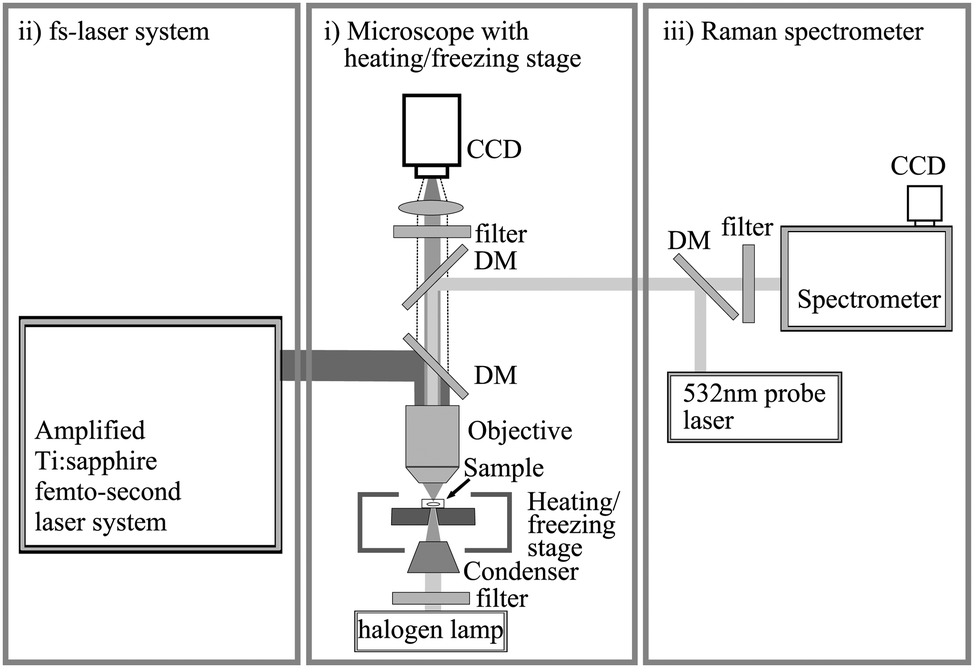

Fig. 3 Simplified scheme of the experimental setup used for this study. See the text for details. DM: dichroic mirror.

(i) The heating/freezing stage (Linkam THMSG 600) is mounted on the microscope and allows for microthermometric measurements in the temperature range between −180 and 600 °C. Temperature calibrations of the stage were performed using synthetic H₂O and H₂O–CO₂ fluid inclusion standards for the triple point of water (0.0 °C), the triple point of CO₂ (−56.6 °C), and the critical point of CO₂ (31.4 °C²⁰). Based on these calibrations, we estimate the accuracy of the temperature measurements at ±0.1 °C around 0 °C, at ±0.2 °C below −20 °C and above 40 °C and at ±0.3 °C above 100 °C. The precision (reproducibility) determined from replicate measurements is ±0.05 °C. Further details are provided in Section S2.2 (ESI†).

(ii) An amplified femtosecond (fs) laser system (Coherent) was used to stimulate vapour bubble nucleation in the metastable liquid state of the inclusions by means of single ultrashort laser pulses. For a detailed description of the setup we refer to the ESI† and to Krüger et al.¹⁶ The experimental setup allows us to stimulate vapour bubble nucleation in selected fluid inclusions at different temperatures under microscopic observation. Subsequent microthermometric measurements can be performed without moving the sample.

(iii) Confocal Raman spectroscopy was used to identify the ice phase in the inclusions in order to determine ice nucleation temperatures. In pure water inclusions the phase transition is not visible from microscopic observations unless a vapour bubble is present that becomes strongly compressed upon ice nucleation. The fiber-coupled Raman setup consists of a 500 mW diode-pumped solid-state single mode laser with 532 nm wavelength and 1 MHz bandwidth (Torus, Laser Quantum), two dichroic mirrors, a spectrometer (Horiba iHR550M CORE 3) and a back-illuminated CCD camera (Horiba SYNAPSE BIVS); for Raman excitation 60 mW was used. Again, a detailed description of the Raman setup is given in the ESI.† The setup allows us to measure Raman spectra at different temperatures under simultaneous observation of the focus position of the excitation beam relative to the fluid inclusions.

2.3. Microthermometric measurements

Using the synthetic pure water inclusions we measured prograde and retrograde liquid–vapour homogenisation temperatures T_h and T_h r, respectively, ice nucleation temperatures T^ice_nr, and ice melting temperatures T^ice_m. Moreover, in low density (ϱ < 925 kg m⁻³) inclusions, we measured the temperatures of spontaneous bubble nucleation, not only the common retrograde T^vap_nr (upon cooling), but also the prograde bubble nucleation T^vap_np, upon heating of inclusions that previously underwent an ice nucleation and melting loop.

The temperatures of the different phase transitions were measured at very low heating and cooling rates respectively to ensure that the sample was in thermal equilibrium with the heating and cooling block of the stage. When approaching the expected phase transition, i.e., for the final 1 or 2 centigrade the temperature was changed in 0.1 centigrade steps with intervals of 10 to 20 seconds in between. The different phase transitions are illustrated in Fig. 4 in a schematic representation of the p–T diagram of water. The phase diagram displays the liquid–vapour (L + V) and liquid–solid (L + S) equilibrium curves, the bubble–nucleation (cavitation) curve (T^vap_nr and T^vap_np), the ice nucleation curve (T^ice_nr) and three liquid-isochores passing through a pressure minimum.

Fig. 4 Schematic p–T phase diagram of water illustrating the different phase transitions observed in this study: liquid–vapour homogenisation (L + V → L), ice nucleation (L → S and L + V → S), final ice melting (L + S → L and L + V + S → L + V) and spontaneous vapour bubble nucleation (L → L + V). Thin solid curves represent three different liquid-isochores. The liquid–vapour equilibrium curve (L + V; solid line) is extended (dotted line) into the supercooled region, while the liquid–solid equilibrium curve (L + S; solid line) is extended to negative pressures (dotted line). The two curves form the upper boundaries of the doubly metastable region in which liquid water is metastable with respect to both vapour and ice. Broad grey lines denote p–T ranges of ice nucleation and spontaneous vapour bubble nucleation, respectively. Arrows indicate pressure increases due to spontaneous or stimulated vapour bubble nucleation as well as due to ice nucleation and subsequent heating. Flash symbols signify laser-induced bubble nucleation.

2.3.1. Prograde and retrograde liquid–vapour homogenisation. Fig. 5 shows a series of inclusion images illustrating prograde (top) and retrograde (bottom) liquid–vapour homogenisation. We started our measurements at 20 °C with inclusions being in a metastable liquid state at negative pressures (tensile stress) and stimulated vapour bubble nucleation by means of single ultrashort laser pulses. When the bubble nucleates, both the pressure and the density of the liquid phase increase and the inclusions transfer into a stable liquid–vapour two-phase state (L → L + V). Upon subsequent heating, the liquid phase expands at the expense of the vapour bubble. The decrease of the bubble size was routinely documented in a series of microphotographs taken at known temperatures. Finally, the vapour bubble collapses and the inclusions homogenise into a stable liquid state (L + V → L) at the (prograde) liquid–vapour homogenisation temperature T_h. Close to T_h, the vapour bubble becomes very small and hardly visible and often it starts moving around in the inclusions, preferably towards the dark corners of the inclusions. Therefore, liquid–vapour homogenisation could not always be observed directly. In these situations, we used a temperature cycling procedure²¹ to precisely determine the temperature at which the bubble finally disappeared.

Fig. 5 Top: Series of inclusion images illustrating prograde liquid–vapour homogenisation. After laser-induced bubble nucleation the inclusion is heated and the vapour bubble becomes smaller due to expansion of the liquid. Close to the homogenisation temperature the bubble starts moving and becomes hardly visible (inside circle). Finally, the bubble collapses and the inclusion homogenises to the liquid. Bottom: Series of inclusion images illustrating retrograde liquid–vapour homogenisation. Observations are the same as for prograde homogenisation.

After T_h measurements the inclusions were cooled to room temperature and vapour bubble nucleation was induced again by means of a femtosecond laser pulse. Subsequently, the inclusions were further cooled to measure the retrograde homogenisation temperature T_h r following the same procedure as described for the T_h measurements. But unlike prograde homogenisation, retrograde homogenisation can only be observed in high-density inclusions, in which T_h r is higher than T^ice_nr, the temperature of ice nucleation. Fig. 4 shows that the isochores of such high-density inclusions intersect the liquid–vapour equilibrium curve (L + V) twice, at T_h and T_h r, respectively. The reproducibility of the measured T_h and T_h r values was routinely checked by duplicate measurements alternately measuring prograde and retrograde homogenisation.

2.3.2. Ice nucleation. At the ice nucleation temperature T^ice_nr the liquid water transforms to solid ice. Again, we started our measurements at 20 °C with inclusions being in a metastable liquid state at negative pressures. Upon cooling the pressure follows the corresponding liquid-isochores to low temperatures (see Fig. 4) until ice spontaneously forms from the supercooled liquid (L → S). Since liquid water instantaneously transforms to ice, the phase transition cannot be observed visually as illustrated in Fig. 6a. Therefore, we used Raman spectroscopy to detect the characteristic change in the Raman spectrum when ice nucleation occurs (Fig. 6b). The Raman spectra were measured using a low-resolution grating (300 grooves per mm) and 1 second integration time, which allowed a ‘real-time’ monitoring of the inclusions during stepwise cooling. Test measurements were performed to ascertain that the 60 mW laser beam used for Raman excitation has no measurable effect on the nucleation of the ice phase as well as on the temperature of the sample. This was done by measurements of T^ice_nr and T^ice_m at saturation pressure and comparing the results obtained with and without laser irradiation of the inclusions.

Fig. 6 (a) Ice nucleation in a supercooled monophase liquid inclusion at negative pressures (L → S). The two images demonstrate that the phase transition cannot be observed visually. (b) Raman spectra of the inclusion shown in (a) illustrating the distinctive change from liquid water to ice. (c) Ice nucleation in the presence of the vapour bubble (L + V → S). The vapour bubble becomes completely compressed due to the larger volume of ice compared to liquid water.

In high-density inclusions featuring retrograde liquid–vapour homogenisation, ice nucleation occurs at positive pressures, while in low-density metastable liquid inclusions nucleation of ice takes place at negative pressures. Since these low-density inclusions do not exhibit retrograde homogenisation, we could also use them to measure T^ice_nr at saturation vapour pressure. To do so, we stimulated vapour bubble nucleation in the metastable liquid and cooled the inclusions along the liquid–vapour equilibrium curve (see Fig. 4). Upon ice nucleation the vapour bubble disappeared again due to the volume expansion of ice relative to liquid water (L + V → S; Fig. 6c).

The nucleation of ice results in an abrupt pressure increase in the inclusions. The pressure in the ice I_h state can be calculated using the equation of state by Feistel and Wagner,²² but since pressure in the inclusions is not measurable, we refrain from exact calculations. To assess the magnitude of the pressure, a rough estimate using Table 11 in ref. 22 is sufficient: in the inclusions with the lowest density of 922 kg m⁻³ ice nucleates at −30.5 °C (see Fig. 9) and the resulting pressure remains below 0.1 MPa (because the density of inclusions is the same as the density of ice at nearly zero pressure at the given temperature). However, in inclusions with ϱ > 942 kg m⁻³ the pressure becomes larger than 200 MPa after ice nucleation, exceeding thereby the range of validity of the ice I_h equation of state. Such high internal pressures can cause irreversible volume changes of the inclusions. Therefore, we routinely re-measured prograde homogenisation temperatures after T^ice_nr and subsequent T^ice_m measurements to check for a potential decrease of the water densities. In the case of irreversible volume changes, the initially measured T^ice_nr values did not reproduce in duplicate measurements but were systematically higher.

2.3.3. Ice melting. After ice nucleation, we heated the samples again to measure ice melting temperatures T^ice_m. The measurements of ice melting temperatures started at T^ice_nr in the positive pressure region of the ice stability field (see Fig. 4). Upon heating, the frozen system moves along the ice isochore p(T|ϱ^ice) and pressure slightly increases until the liquid–solid equilibrium is reached, where the ice starts melting at the initial ice melting temperature T^ice_m(i) (S → S + L), note that T^ice_m(i) depends on pressure, i.e., on the density of inclusions. With further increase of the temperature, the system moves down along the melting curve and with some temperature delay a phase boundary between the ice and liquid phases becomes visible, which can be used as a maximum estimate of the initial ice melting temperature. Due to relatively large uncertainties in determining the initial ice melting temperatures, we did not systematically measure T^ice_m(i) in the present study. Upon further heating, ice melts continuously and final melting is achieved at a temperature T^ice_m (L + S → L), which occurs at negative pressures, ideally at the intersection of the L + S curve with the corresponding liquid-isochore of the inclusions, as indicated in Fig. 4. After the final ice melting the inclusions were again in a metastable liquid state and we subsequently re-measured T_h to check whether the inclusion volumes have changed due to ice nucleation.

The inclusions with the lowest water densities analysed in this study (T_h > 140 °C) allowed us to measure the ice melting temperature under three-phase conditions (see Fig. 7b). For this purpose, we used the femtosecond laser pulses to stimulate vapour bubble nucleation during melting at −0.1 °C in the presence of liquid water and ice (L + S → L + S + V). In the inclusion shown in Fig. 7b, the final ice melting was measured between 0.0 and +0.1 °C (L + V + S → L + V) as expected for pure water inclusions.

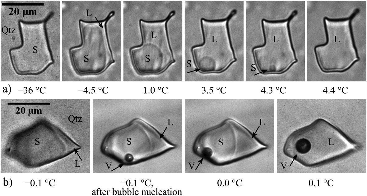Fig. 7 (a) Series of inclusion images illustrating ice melting in the absence of the vapour bubble. Ice melting proceeds continuously after reaching the L + S equilibrium curve. Final ice melting occurred at positive temperatures in the metastable liquid region (L + S → L). (b) Final ice melting at saturation pressure after stimulating vapour bubble nucleation (L + V + S → L + V).

2.3.4. Spontaneous vapour bubble nucleation. Two of our quartz samples contained low-density fluid inclusions that were in a stable liquid–vapour two-phase state at room temperature due to spontaneous nucleation of the vapour bubble (L → L + V). We started the measurements of retrograde bubble nucleation temperatures T^vap_nr first by heating the samples in order to re-homogenise the inclusions at temperatures between 145 and 151 °C (L + V → L). Upon subsequent cooling the pressure in the inclusions follows the corresponding liquid-isochore into the metastable region up to the spontaneous nucleation of the vapour bubble. In addition to retrograde bubble nucleation (upon cooling) we also observed prograde vapour bubble nucleation (upon heating) in the same inclusions. Starting again with a liquid–vapour two-phase state, the inclusions were cooled along the liquid–vapour equilibrium curve until ice nucleated. Now, the vapour bubble vanished either directly upon ice nucleation (L + V → S) or afterwards due to a slight expansion of ice upon subsequent heating (L + V → S + V → S). We continued heating until ice started to melt at the liquid–solid equilibrium (S → S + L). Upon further heating the pressure in the inclusions follows the ice melting curve into the metastable region until all the ice had melted at T^ice_m (L + S→L). Now, the inclusions were again in a metastable liquid state and pressure was determined by the liquid-isochore. Finally, upon further heating, we observed spontaneous prograde vapour bubble nucleation (L → L + V) at T^vap_np values that were systematically lower than retrograde bubble nucleation temperatures T^vap_nr. Measurements of T^vap_nr and T^vap_np were performed at a constant cooling and heating rate of 2 centigrade per minute.

2.4. Basics of data analysis

2.4.1. IAPWS-95. Fluid inclusion microthermometry provides information only on the temperature of phase transitions while pressure and density need to be calculated based on an adequate equation of state. In this study, we used the IAPWS-95 formulation of Wagner and Pruss¹¹ that provides the Helmholtz energy of the liquid and gaseous phases from which the p–V–T properties of an isochoric pure water system can be derived. The validity range of the formulation is between 250 and 1273 K and from 0 to 1000 MPa.

In the first place, we used the IAPWS-95 formulation to calculate the density of the liquid phase at saturation pressure, i.e., along the liquid–vapour equilibrium curve. At this point, we note that in addition to the IAPWS-95 formulation, Wagner and Pruss also reported a polynomial function that can be used alternatively to calculate liquid-densities along the liquid–vapour curve (eqn (2.6), Section 2.3.1¹¹). However, since this polynomial is an empirical fit to experimental data above 0 °C, it covers only the stable part of the liquid–vapour curve and should not be extrapolated into the supercooled metastable region. A comparison of the two modes of calculation revealed increasing divergence of the liquid densities below −20 °C, with lower densities resulting from IAPWS-95.

The IAPWS-95 formulation is considered to exhibit ‘reasonable’ behaviour when extrapolated into the metastable liquid region (Section 7.3.2¹¹). It allows us to extrapolate the liquid-isochores into the metastable region and to calculate the liquid-spinodal. Similar to the ‘stability limit conjecture’,⁵ IAPWS-95 assumes a negative slope of the TMD line in the metastable region, and, as a consequence, the spinodal turns up towards positive pressures at low temperatures.

Although IAPWS-95 does not provide any information about the solid states of water, Wagner and Pruss gave a polynomial function describing the p–T trend of the ice melting curve (I_h) (eqn (2.16), Section 2.4.1¹¹) derived from Wagner et al.²³ The curve is based on a fit to experimental data, including a few measurements of Henderson and Speedy,²⁴ providing ice melting temperatures in the metastable region down to −22.8 MPa. Due to the lack of experimental data at higher tensile stress, we extrapolated the ice melting curve further into the metastable region for comparison with our new ice melting data.

2.4.2. Effect of surface tension. The temperature at which the liquid–vapour equilibrium curve intersects the liquid-isochore (see Fig. 4) determines the bulk density of the water in the inclusions and is commonly referred to as the liquid–vapour homogenisation temperature T_h. Strictly speaking, however, this definition of T_h holds true only for infinitely large systems since it does not account for the volume-dependent effect of surface tension on liquid–vapour homogenisation. Henceforth, we will therefore use the term T_h∞ to denote the intersection of the liquid–vapour equilibrium curve with the liquid-isochore. This T_h∞ determines the actual bulk density ϱ_bulk of the liquid water in the inclusions. While the effect of surface tension is negligible in macroscopic systems, it becomes significant in microscopic systems like fluid inclusions, particularly for low homogenisation temperatures, i.e., at high water densities. Here, the actually observed homogenisation temperature T_h obs depends not only on the density but also on the size of the inclusions as demonstrated by Fall et al.²⁵ This means that besides T_h obs an additional volume measurement is required to determine the density of the inclusions. For practical reasons, we do not measure the volume V of the inclusions (cf. Stoller et al.²⁶). Instead, we determine the volume of the spherical vapour bubble based on radius measurements r(T) at known temperatures (see Section 2.4.4. below). For the calculations of T_h∞ (and thus ϱ_bulk) and the inclusion volume V we used the thermodynamic model of Marti et al.¹⁷ that accounts for the effect of surface tension on liquid–vapour equilibria in isochoric systems. The model relies on the minimisation of the Helmholtz energy of the system derived from the IAPWS-95 formulation, and predicts the thermodynamic state, the vapour bubble radius, the density and pressure of the liquid and vapour phases at a given temperature, and the volume and bulk density of the system. For inclusions analysed in this study, the temperature differences between T_h obs and T_h∞ were up to 1.8 °C. A schematic p–T diagram illustrating the effect of surface tension on liquid–vapour homogenisation is shown in Fig. S2 (ESI†).

2.4.3. Deviation from the isochoric system. Fluid inclusions are commonly regarded as isochoric systems, in which the pressure p(T) is defined by a liquid-isochore. In the present study, however, we applied a correction to account for the temperature-dependent volume change of the quartz crystal hosting the inclusions using expansion coefficients α of Desai.²⁷ The pressure p(T) in the inclusions now follows a “pseudo-isochoric” curve. Although the volume changes of the quartz host are relatively small, they result in a significant shift of the retrograde homogenisation temperature compared to the isochoric system. A schematic p–T diagram illustrating the difference between an isochoric and a quartz-confined system with respect to retrograde homogenisation is shown in Fig. S3 (ESI†).

2.4.4. Bubble radius measurements. The radius of the vapour bubble was determined based on microphotographs taken at different temperatures assuming a spherical bubble.²⁸ The inclusions analysed in this study, however, were often flat and the bubble diameter, particularly in ‘low-density’ inclusions exceeded the extension of the inclusions in the z-direction, which results in an oblate shape of the bubble and a radius that is apparently too large. To check whether or not the vapour bubble is spherical at a specific temperature we analysed the changes in the measured bubble radii as a function of temperature. Fig. 8a shows the example of a ‘low-density’ inclusion with a spherical vapour bubble in the entire temperature range between T_h obs and T^ice_nr. The solid curve represents the best fit of the radius measurements and predicts the theoretical evolution of the bubble radius for an inclusion volume of 210 μm³. In contrast, Fig. 8b shows another ‘low-density’ inclusion, in which the bubble becomes spherical only at radii smaller than 1.7 μm, i.e., at temperatures above 60 °C and below −20 °C, respectively. At temperatures in between the measured bubble radii are systematically larger than the theoretical radii predicted for an inclusion volume of 410 μm³, which indicates deformation of the bubble due to the confining inclusion walls. We performed these radius analyses for all inclusions in this study in order to eliminate a potential source of error in the determination of the inclusion volume V, and thus T_h∞, T_h r∞, and the bulk density ϱ_bulk. The accuracy of the radius measurements is estimated to be ±0.15 μm. The precision of the measurements is ±0.05 μm reflecting the deviation of the measured bubble radii from the best-fit curve of the theoretical radius evolution.

Fig. 8 Comparison of bubble radius measurements (dots) with the theoretical radius evolution (solid curve). Error bars indicate the estimated accuracy of the radius measurements of ±0.15 μm. (a) Example of an inclusion with a spherical vapour bubble in the entire temperature range. The volume of the inclusion was determined to be 210 ± 60 μm³. (b) Example of an inclusion in which the bubble is obviously oblate if the radius exceeds 1.7 μm. The volume of the inclusion was determined to be 360 ± 90 μm³. In both examples shown, T^ice_nr occurs before T_h r obs.

Fig. 9 ϱ–T diagram illustrating the results of the fluid inclusion measurements. T^ice_nr: ice nucleation in the absence of the vapour phase (L → S). T^ice_m: final ice melting in the absence of the vapour phase (L + S → L). T_h∞ and T_h r∞: prograde and retrograde liquid–vapour homogenisation (L + V → L). T^vap_nr and T^vap_np: spontaneous retrograde and prograde vapour bubble nucleation (L → L + V). The results of previous experimental studies are plotted for comparison. L + V: liquid–vapour equilibrium curve (IAPWS-95). L + S: liquid–solid equilibrium curve.²³ Dashed line: liquid-spinodal (IAPWS-95). Grey solid nearly horizontal lines: pseudo-isochore curves. Dash-dotted line: density of ice at zero pressure.²²

3. Results

A graphical representation of the results obtained in this study is shown in Fig. 9 and displays T_h∞, T_h r∞, T^ice_nr (only L → S), T^ice_m, T^vap_nr and T^vap_np as a function of density. The reason for using a ϱ–T representation instead of the more familiar p–T diagram is that we have an accurate measure for the density of the inclusions via T_h obs and the bubble radius r(T), whereas the pressure inside the inclusions needs to be calculated by extrapolation of the IAPWS-95 formulation into the metastable region. The diagram displays additional experimental data from previous studies^{10,12,13,29–31} for comparison with our new data. The liquid–vapour equilibrium curve (L + V) and the liquid-spinodal were derived from IAPWS-95,¹¹ and the liquid–solid equilibrium curve (L + S) was derived from the polynomial function given by Wagner et al.²³ Finally, the diagram displays three pseudo-isochores (with slight negative slopes) that intersect the liquid–vapour equilibrium curve at T_h∞ values of 50, 90 and 150 °C (with bulk densities of 988.0, 965.3 and 917.0 kg m⁻³, respectively). Numerical values of our experimental data are reported in Tables 1–3.

Table 1 Results of the microthermometric measurements of prograde and retrograde liquid–vapour homogenisation T_h obs and T_h r obs, (retrograde) ice nucleation T^ice_nr, and final ice melting T^ice_m of 26 fluid inclusions. Temperature accuracies are estimated based on the calibration of the heating/freezing stage. Vapour bubble radii r(T) refer to a temperature of 20 °C and were derived from theoretical radius curves fitted to the measured values. T_h∞, T_h r∞ and the volume V of the inclusions were calculated using the model of Marti et al.¹⁷ Due to the small size of the inclusions, the uncertainty of the bubble radius measurements (±0.15 μm) results in large relative errors of the inclusion volumes. However, the effect of the volume error on T_h∞ and T_h r∞ is small. The overall uncertainty of T_h∞ and T_h r∞ given in the table comprises the error relating to the temperature accuracy of the stage, the error resulting from the volume uncertainty, and an additional uncertainty associated with the vapour bubble collapse (see Section S2.4.2, ESI). The density of water at T^ice_nr and at T^ice_m was determined from T_h∞ by applying a correction for the temperature-dependent volume change of the quartz host. Note that the densities assigned to T^ice_m were determined from re-measurements of T_h obs performed after ice melting to account for potential volume increases of the inclusions resulting from ice nucleation. In particular, high-density inclusions with T_h∞ < 90 °C were often subject to irreversible volume changes, and thus, the densities at T^ice_m did not relate to the initial T_h∞ values reported in the table. For low-density inclusions that did not stretch due to ice nucleation Table 1 reports only the lowest T^ice_nr values measured in each inclusion considering these minimum temperatures as the closest approximation to homogeneous ice nucleation

Inclusion	T h obs (L + V → L) (°C)	T h r obs (L + V → L) (°C)	T ^icenr (L → S) ±0.2 °C	T ^icem (L + S → L) ±0.1 °C	r(@20 °C) ±0.15 μm	T h∞ (°C)	T h r∞ (°C)	V (μm^3)	ϱ bulk(Th∞) (kg m^−3)	ϱ(T^icenr) (kg m^−3)	ϱ(T^icem) (kg m^−3)
13-2-3	28.7 ± 0.1	−12.4 ± 0.1	−43.3	0.4	0.61	30.18^+0.46−0.32	−13.63^−0.39+0.29	450^−260+400	995.55^−0.14+0.10	997.75^−0.13+0.09	995.23^−0.12+0.10
13-2-2	29.8 ± 0.1	−13.2 ± 0.1	−43.3	0.4	0.46	31.64^+0.72−0.46	−14.70^−0.60+0.38	160^−110+230	995.10^−0.23+0.15	997.34^−0.21+0.13	994.53^−0.18+0.11
13-3-3	36.4 ± 0.2	−16.8 ± 0.1	−43.0	0.6	0.70	37.67^+0.45−0.37	−17.80^−0.29+0.23	330^−170+260	993.05^−0.16+0.14	995.44^−0.15+0.12	993.37^−0.15+0.12
13-3-4	45.0 ± 0.2	−21.5 ± 0.2	−42.4	1.0	0.55	46.42^+0.58−0.43	−22.55^−0.37+0.37	90^−60+100	989.57^−0.25+0.19	992.22^−0.23+0.17	989.86^−0.23+0.17
2-2-6	49.2 ± 0.2	−23.2 ± 0.2	−42.1	1.1	0.99	50.09^+0.31−0.29	−23.84^−0.28+0.26	430^−160+250	987.96^−0.14+0.13	990.70^−0.13+0.12	985.90^−0.12+0.11
14-1-4	51.4 ± 0.2	−24.2 ± 0.2	−42.3	1.2	0.51	52.85^+0.62−0.46	−25.22^−0.49+0.37	70^−30+70	986.68^−0.29+0.22	989.51^−0.28+0.20	987.87^−0.27+0.20
14-1-3	61.8 ± 0.2	−28.6 ± 0.2	−41.1	1.8	0.61	63.00^+0.47−0.39	−29.39^−0.37+0.32	60^−30+60	981.59^−0.25+0.21	984.68^−0.26+0.18	981.45^−0.24+0.20
2-1-3	71.8 ± 0.2	−31.9 ± 0.2	−40.4	2.1	0.91	72.64^+0.32−0.29	−32.42^−0.27+0.25	160^−70+90	976.21^−0.19+0.17	979.55^−0.18+0.16	978.51^−0.18+0.16
2-1-3c	74.5 ± 0.2	−32.9 ± 0.2	−40.1	2.1	0.91	75.34^+0.31−0.30	−33.42^−0.27+0.25	150^−60+90	974.61^−0.18+0.18	978.02^−0.18+0.17	977.00^−0.17+0.17
8-1-4	79.9 ± 0.2	−34.9 ± 0.2	−39.7	2.3	1.60	80.44^+0.24−0.23	−35.21^−0.22+0.22	690^−180+230	971.49^−0.15+0.15	975.06^−0.16+0.12	973.87^−0.14+0.14
2-1-4c	81.6 ± 0.2	−35.1 ± 0.2	−39.8	2.2	1.20	82.26^+0.27−0.26	−35.48^−0.24+0.23	280^−90+120	970.35^−0.17+0.16	973.94^−0.16+0.16	972.94^−0.16+0.16
8-1-1	88.8 ± 0.2	−36.8 ± 0.2	−38.5	2.8	1.05	89.52^+0.28−0.27	−37.19^−0.24+0.23	160^−60+80	965.62^−0.19+0.18	969.37^−0.17+0.19	968.24^−0.18+0.17
8-1-7	91.7 ± 0.2	Not observed	−37.7	3.0	2.04	92.42^+0.28−0.27	—	150^−60+70	963.66^−0.19+0.18	967.49^−0.19+0.18	966.55^−0.19+0.17
8-2-7	94.8 ± 0.2	n.o.	−37.3	3.1	1.35	95.38^+0.25−0.25	—	310^−90+100	961.61^−0.18+0.17	965.51^−0.17+0.17	963.50^−0.17+0.17
10-5-6	111.5 ± 0.3	n.o.	−36.1	4.4	1.14	112.14^+0.36−0.36	—	140^−50+60	949.31^−0.28+0.28	953.62^−0.27+0.27	952.74^−0.27+0.27
10-5-4	113.5 ± 0.3	n.o.	−35.9	4.5	1.18	114.11^+0.37−0.35	—	150^−50+60	947.78^−0.29+0.27	952.13^−0.28+0.27	951.26^−0.27+0.26
4-2-6	115.2 ± 0.3	n.o.	−36.1	4.6	1.07	115.86^+0.38−0.36	—	100^−40+50	946.41^−0.30+0.28	950.81^−0.29+0.28	949.94^−0.29+0.27
4-2-4	120.9 ± 0.3	n.o.	−35.2	5.1	1.19	121.50^+0.36−0.35	—	130^−50+60	941.46^−0.30+0.28	946.42^−0.29+0.28	945.58^−0.29+0.27
4-1-3	126.7 ± 0.3	n.o.	−34.1	5.3	1.12	127.32^+0.37−0.35	—	100^−30+50	937.09^−0.31+0.30	941.77^−0.30+0.29	940.94^−0.30+0.29
7-7-10	127.4 ± 0.3	n.o.	−34.4	5.4	1.20	127.99^+0.36−0.35	—	130^−40+50	936.53^−0.30+0.29	941.21^−0.30+0.28	940.40^−0.29+0.28
4-1-7	132.1 ± 0.3	n.o.	−33.1	5.7	1.80	132.53^+0.33−0.32	—	400^−90+100	932.67^−0.28+0.28	937.44^−0.27+0.27	936.65^−0.27+0.27
4-1-6	135.2 ± 0.3	n.o.	−32.3	6.0	1.11	135.82^+0.37−0.36	—	90^−30+40	929.83^−0.32+0.31	934.66^−0.31+0.30	933.89^−0.31+0.30
4-1-1	137.8 ± 0.3	n.o.	−32.1	6.1	1.82	138.22^+0.33−0.32	—	380^−90+100	927.71^−0.29+0.29	932.60^−0.28+0.28	931.84^−0.28+0.28
4-1-4	141.9 ± 0.3	n.o.	−31.4	6.4	1.52	142.38^+0.34−0.33	—	210^−60+70	924.00^−0.31+0.30	928.98^−0.30+0.29	928.23^−0.30+0.29
6-2-4	148.0 ± 0.3	n.o.	−30.7	6.7	1.86	148.41^+0.33−0.32	—	360^−80+100	918.49^−0.30+0.30	923.60^−0.30+0.29	922.88^−0.29+0.30
6-2-1	149.7 ± 0.3	n.o.	−30.5	6.8	1.55	150.17^+0.34−0.33	—	201^−53+65	916.85^−0.32+0.31	922.00^−0.31+0.30	921.28^−0.31+0.30

---

Table 2 Ice nucleation temperatures T^ice_nr of 23 inclusions measured at saturation pressure, i.e. in the presence of the vapour bubble (L + V → S). We report the lowest T^ice_nr values measured in each inclusion. In addition, the table lists T_h∞, the volume V of the inclusions, and the bubble radius r(T) at T^ice_nr

Inclusion	T ^icenr (L + V → S) ±0.2 °C	T h∞ (°C)	V (μm^3)	r(T^icenr) ±0.15 μm
7-2-1	−37.8	145.75^+0.33−0.33	250^−60+80	1.36
7-6-1	−38.1	145.70^+0.32−0.32	420^−90+100	1.64
7-6-6	−38.3	146.10^+0.37−0.35	80^−30+40	0.94
7-6-5	−38.3	146.14^+0.35−0.34	120^−40+50	1.06
7-6-3	−38.1	146.21^+0.33−0.32	360^−80+100	1.52
7-6-9	−38.5	146.45^+0.33−0.33	250^−60+80	1.39
7-6-7	−38.5	147.12^+0.38−0.36	70^−30+30	0.90
7-2-2	−37.9	147.14^+0.33−0.32	280^−70+80	1.42
7-6-4	−38.4	147.14^+0.34−0.33	270^−70+80	1.40
6-2-4	−38.4	148.31^+0.33−0.32	360^−80+100	1.59
6-2-7	−38.7	148.47^+0.36−0.35	100^−30+40	1.02
6-2-5	−39.0	148.62^+0.37−0.36	70^−20+30	0.90
6-2-6	−39.1	148.87^+0.36−0.35	100^−30+40	1.03
6-3-8	−39.5	149.71^+0.35−0.34	140^−40+50	1.12
6-3-9	−39.6	150.01^+0.35−0.34	140^−40+50	1.14
6-2-3	−38.7	150.21^+0.37−0.36	70^−30+30	0.91
6-2-2	−38.8	151.04^+0.38−0.36	60^−20+30	0.87
6-3-13	−39.6	150.99^+0.35−0.34	120^−40+50	1.10
6-2-1	−38.9	150.92^+0.35−0.34	130^−40+50	1.13
4-2-4	−39.2	121.50^+0.36−0.35	130^−50+60	0.86
4-2-6	−39.1	115.86^+0.38−0.36	100^−40+50	0.72
8-2-7	−39.2	95.38^+0.25−0.25	310^−90+100	0.55
10-5-6	−38.2	112.14^+0.36−0.36	140^−50+60	0.71

---

Table 3 Retrograde and prograde bubble nucleation temperatures T^vap_nr and T^vap_np of 22 inclusions. The tabulated T^vap_nr values represent the lowest temperatures measured for each inclusion, whereas for prograde bubble nucleation the highest T^vap_np values are reported. In addition, the table lists the corresponding T_h∞ values, the inclusion volume V, the bubble radius r at 20 °C as well as the water densities ϱ(T) at T_h∞, T^vap_nr and T^vap_np, respectively

Inclusion	T ^vapnr (L → L + V) ±0.2 °C	T ^vapnp (L → L + V) ±0.1 °C	r(20 °C) ±0.15 μm	T h∞ (°C)	V (μm^3)	ϱ bulk(Th∞) (kg m^−3)	ϱ(T^vapnr) (kg m^−3)	ϱ(T^vapnp) (kg m^−3)
7-6-2	53.7	29.6	1.86	145.21^+0.33−0.32	370^−80+100	921.43^−0.30+0.30	924.50^−0.29+0.29	925.17^−0.29+0.29
7-2-1	55.9	22.7	1.64	145.75^+0.33−0.33	250^−60+80	920.94^−0.31+0.30	923.96^−0.30+0.29	924.74^−0.31+0.49
7-6-1	59.7	22.8	1.94	145.70^+0.32−0.32	420^−90+100	920.99^−0.30+0.29	923.89^−0.29+0.28	924.91^−0.29+0.29
7-6-10	53.8	29.6	1.82	145.72^+0.33−0.32	350^−80+100	920.97^−0.30+0.30	924.05^−0.29+0.29	924.72^−0.29+0.29
7-6-6	64.7	17.2	1.13	146.10^+0.37−0.35	80^−30+40	920.62^−0.34+0.32	923.39^−0.33+0.31	924.69^−0.33+0.31
7-6-5	65.5	17.1	1.28	146.14^+0.35−0.34	120^−40+50	920.58^−0.32+0.31	923.32^−0.31+0.30	924.66^−0.31+0.30
7-6-3	63.3	17.3	1.85	146.21^+0.33−0.32	360^−80+100	920.52^−0.30+0.30	923.33^−0.29+0.29	924.59^−0.29+0.29
7-6-9	62.2	23.8	1.63	146.45^+0.33−0.33	250^−60+80	920.30^−0.31+0.30	923.15^−0.30+0.29	924.21^−0.30+0.29
7-6-8	52.9	26.2	2.15	146.57^+0.32−0.32	560^−110+130	920.19^−0.29+0.29	923.32^−0.28+0.28	924.05^−0.29+0.28
7-6-7	62.9	18.1	1.06	147.12^+0.38−0.36	70^−30+30	919.68^−0.35+0.33	922.53^−0.33+0.32	923.76^−0.34+0.32
7-2-2	61.8	24.3	1.70	147.14^+0.33−0.32	280^−70+80	919.66^−0.31+0.30	922.55^−0.30+0.29	923.59^−0.30+0.29
7-6-4	68.8	16.7	1.68	147.14^+0.34−0.33	270^−70+80	919.66^−0.31+0.30	922.33^−0.30+0.29	923.77^−0.30+0.29
6-2-4	64.4	n.o.	1.88	148.31^+0.33−0.32	360^−80+100	918.58^−0.30+0.30	921.43^−0.29+0.29	—
6-2-7	64.8	20.1	1.20	148.47^+0.36−0.35	100^−30+40	918.43^−0.33+0.32	921.27^−0.32+0.31	922.50^−0.32+0.31
6-2-5	54.4	29.1	1.07	148.62^+0.37−0.36	70^−20+30	918.29^−0.35+0.33	921.44^−0.34+0.32	922.14^−0.34+0.32
6-2-6	59.1	29.5	1.20	148.87^+0.36−0.35	100^−30+40	918.06^−0.33+0.32	921.08^−0.32+0.31	921.91^−0.32+0.31
6-3-8	69.8	19.5	1.38	149.71^+0.35−0.34	140^−40+50	917.28^−0.32+0.31	920.00^−0.31+0.30	921.40^−0.31+0.31
6-3-9	65.9	18.2	1.38	150.01^+0.35−0.34	140^−40+50	917.00^−0.32+0.32	919.85^−0.31+0.30	921.16^−0.31+0.31
6-2-3	65.2	22.6	1.09	150.21^+0.37−0.36	70^−30+30	916.81^−0.35+0.33	919.69^−0.34+0.32	920.87^−0.34+0.32
6-2-2	72.8	16.8	1.01	151.04^+0.38−0.36	60^−20+30	916.03^−0.36+0.34	918.70^−0.35+0.33	920.25^−0.35+0.33
6-3-13	71.8	n.o.	1.29	150.99^+0.35−0.34	120^−40+50	916.41^−0.33+0.32	919.10^−0.32+0.31	—
6-2-1	72.8	12.6	1.35	150.92^+0.35−0.34	130^−40+50	916.15^−0.33+0.32	918.81^−0.32+0.31	920.46^−0.32+0.31

---

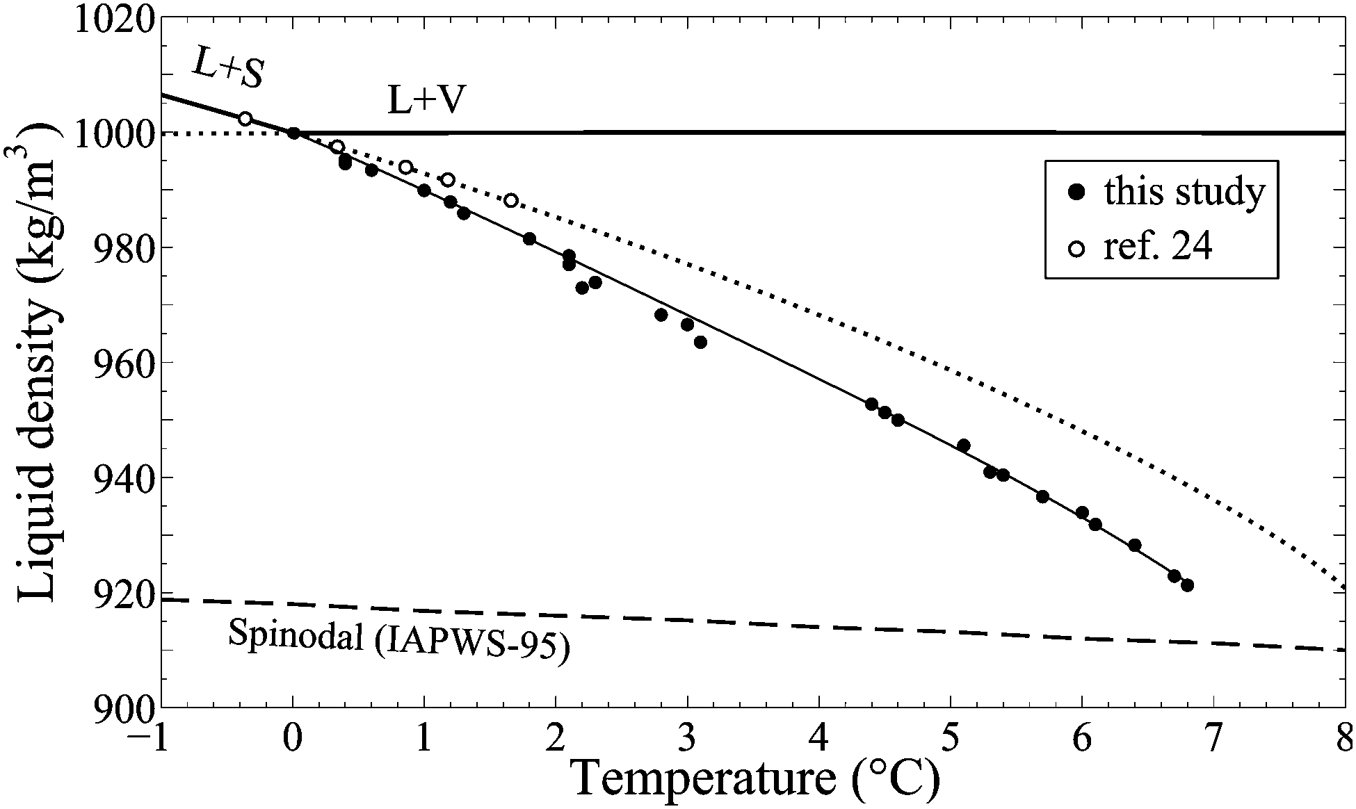
3.1. Liquid–vapour homogenisation data

Fig. 9 displays the T_h∞ and T_h r∞ data of prograde and retrograde liquid–vapour homogenisation, respectively, which by definition are plotted on the liquid–vapour equilibrium curve (L + V) and hence determine the bulk density of the water in the inclusions. The densities ϱ_bulk derived from prograde liquid–vapour homogenisation are used here as reference values to characterise the inclusions. They range from 996 to 916 kg m⁻³. By applying a correction to ϱ_bulk for the temperature-dependent volume change of the quartz host, we obtained ϱ(T), the density of an inclusion at any other temperature, namely at T^ice_nr, T^ice_m, T^vap_np and T^vap_nr. Retrograde liquid–vapour homogenisation was observed only in high-density inclusions with ϱ_bulk greater than 965 kg m⁻³, corresponding to T_h∞ values below 90 °C. The lowest T_h r∞ value determined in this study was −37.2 °C.

3.2. Ice nucleation data

In high-density inclusions with T_h∞ < 90 °C, ice nucleation commonly resulted in irreversible volume changes, and thus, T^ice_nr systematically increased in replicate measurements. This effect did not occur in low-density inclusions, in which case, T^ice_nr was typically reproduced within ±0.5 °C. In Table 1 and Fig. 9, we report only the lowest T^ice_nr value measured in each inclusion considering these minimum temperatures as the closest approximation to homogeneous ice nucleation. Apart from a slight scatter, the data points (eight spoked asterisks) shown in Fig. 9 indicate a linear increase of T^ice_nr with decreasing density in the range covered in this study. (Sorry for the lack of data points just below the saturation curve.) For a more detailed view of the ice nucleation data on an enlarged scale we refer to Fig. S4 (ESI†). We report an ice nucleation line (L → S) derived from a linear fit to our data:

ϱ(T^ice_nr) = −5.8481T + 743.53

with ϱ(T^ice_nr) in kg m⁻³ and T in °C, validity range from −43.3 to −30.5 °C. In addition to our own ice nucleation data, Fig. 9 displays independent measurements of Kanno and Miyata³⁰ at high densities, i.e., at positive pressures. Since Kanno and Miyata reported the p–T data of ice nucleation we converted them to ϱ–T using the IAPWS-95 formulation. The agreement between the two data sets is quite good. Although the formation of ice in stretched water has been observed by several authors,^24,32–34 quantitative data of T^ice_nr in the doubly metastable region are scarce and considerably higher than those measured in this study.

The ice nucleation line intersects the liquid–vapour equilibrium curve at −38.2 °C, providing an estimate of the expected ice nucleation temperature T^ice_nr at saturation pressure (L + V → S). In comparison to this, the real T^ice_nr measurements performed in the presence of the vapour bubble (not shown in Fig. 9) yielded slightly lower values, ranging between −37.8 and −39.6 °C (see Fig. S5, ESI†). Although these measurements suggest a potential effect of the vapour bubble on ice nucleation temperatures, we found only a weak correlation between T^ice_nr and the bubble radius r at T^ice_nr (see Fig. S6, ESI†). Replicate measurements of individual inclusions reproduced, with few exceptions, within ±0.5 °C. Again, Table 2 and Fig. S5 and S6 (ESI†) report the lowest T^ice_nr (L + V → S) values measured in each inclusion.

At −36.2 °C, Fig. 9 and Fig. S4 (ESI†) additionally show an intersection of the ice nucleation line with the liquid-spinodal predicted by IAPWS-95 (dashed curve). As a result, ice nucleation temperatures measured in low-density inclusions (ϱ(T^ice_nr) < 955 kg m⁻³) are plotted on the left hand side of the spinodal i.e., within the IAPWS-95 defined region of the unstable liquid. Therefore, IAPWS-95 cannot provide any pressures at T^ice_nr for these low-density inclusions, which is another reason for presenting our data in a ϱ–T diagram. It should be noted that we did not observe any indication for a change in the state of liquid water above T^ice_nr. Moreover, we found that the application of femtosecond laser pulses in the doubly metastable region, even close to T^ice_nr, resulted in vapour bubble nucleation but never stimulated ice nucleation. We therefore conclude that ice nucleation in fluid inclusions is not triggered by bubble nucleation as it was observed by Barrow et al.³⁴ in Berthelot tube experiments.

3.3. Final ice melting data

The results of final ice melting measurements (dots) illustrated in Fig. 9 indicate an increase of T^ice_m with decreasing density ϱ(T^ice_m). For comparison, the diagram also displays a reference ice-melting curve derived by extrapolation of eqn (2.16)¹¹ into the metastable region. Again, the initial p–T curve was converted to a ϱ–T curve using the IAPWS-95 formulation. Our fluid inclusion data show significant deviations from the extrapolated T^ice_m curve, which will be discussed in detail in Section 4.3. At densities around 970 kg m⁻³, we also observed a slight step in our ice melting data, which is supposed to have no physical meaning. Repeated measurements of these inclusions revealed significant variations of T_h obs after T^ice_m measurements that were not linked to corresponding changes in T^ice_m. Therefore, we do not consider these data reliable. At saturation pressure, i.e., in the presence of the vapour bubble, T^ice_m was measured at 0.0 ± 0.1 °C, which is in agreement with pure water inclusions. The maximum temperature of the final ice melting was measured to be +6.8 °C, which corroborates a previously reported temperature of +6.5 °C observed by Roedder³³ in metastable fluid inclusions.

3.4. Spontaneous bubble nucleation data

In the present study, spontaneous vapour bubble nucleation (or cavitation) occurred only in inclusions with T_h∞ > 145 °C. Replicate measurements of T^vap_nr and T^vap_np revealed a reproducibility within ±3 °C for individual inclusions. A comparison of different inclusions of similar densities (i.e., similar T_h∞ values), however, revealed larger variations of up to 10 °C, though we found no correlation with the inclusion volume in the range of inclusion sizes we were looking at. In Table 3 and Fig. 9, we report the lowest T^vap_nr values measured in each inclusion and the highest values of T^vap_np, respectively. Retrograde bubble nucleation was observed 80 °C to 90 °C below T_h∞, far away from the predicted liquid-spinodal. T^vap_np can be observed only in a narrow range of inclusion densities ϱ_bulk between 921.4 and 916.1 kg m⁻³, corresponding to T_h∞ values between 145.2 and 150.9 °C. At lower bulk densities, i.e., higher T_h∞ prograde bubble nucleation cannot be measured anymore because in these inclusions the ice phase does not fully compensate the bubble volume, and as a consequence ice melting occurs solely at saturation pressure and not at negative pressures in the metastable region. The temperature difference between T^vap_nr and T^vap_np tends to decrease with increasing density (decreasing T_h∞). An interpolation of our data suggests that T^vap_nr and T^vap_np become equal at around 40 °C. In the present study, the highest T_h∞ value of an inclusion that did not show spontaneous bubble nucleation was determined to be 142.4 °C (924.0 kg m⁻³).

In addition, Fig. 9 also displays some T^vap_nr data from previous studies.^{10,12,13,29,31} For the calculation of the corresponding ϱ(T^vap_nr) from these studies we treated T_h obs equal to T_h∞ since they only report T_h obs values. In fact in inclusions with ϱ < 930 kg m⁻³, the relative difference in ϱ_bulk resulting from the difference between T_h obs and T_h∞ is less than 0.05%, and thus, is negligible. In contrast to our own data, the T^vap_nr values reported in ref. 10, 29 and Table 1 of ref. 13 show a much larger scatter by several tens of degrees for different inclusions of similar densities. We therefore display only the lowest of these values in Fig. 9. The locus of the nucleation data points in the ϱ–T plane appears to form a bubble nucleation (cavitation) curve that exhibits a maximum at around 40 °C (see Discussion in Section 4.4).

4. Discussion

4.1. Evaluation of saturation liquid densities in the supercooled region

Retrograde liquid–vapour homogenisation temperatures provide information on the ϱ–T trend of the liquid–vapour equilibrium curve in the supercooled region. To evaluate our data, we calculated T_h r∞ based on T_h r obs and the reference bubble radius r(20 °C) of the inclusions. The corresponding (prograde) T_h∞ values were calculated accordingly from T_h obs using the same reference bubble radius. In this way, we obtained two independent densities for the same inclusion. In Fig. 10, we compare the T_h∞–T_h r∞ pairs obtained from high-density inclusions with a reference curve derived from IAPWS-95. To make the isochoric IAPWS-95 curve (dashed line) comparable to our fluid inclusion data, we applied a correction for the temperature-dependent volume change of the quartz host, which shifts the predicted T_h∞–T_h r∞ curve to the left (solid line). The starting points of the two curves are defined by the temperatures at which T_h∞ equals T_h r∞ (open circles). In the isochoric system this is at 4.0 °C, i.e. at the temperature of maximum density (TMD), whereas in the case of a quartz-confined system, the starting point is at 6.15 °C.³⁵ According to IAPWS-95 both curves end at −39.6 °C (vertical dash-dotted line), representing the temperature at which the liquid-spinodal intersects the liquid–vapour curve in the supercooled region. We recall that IAPWS-95 does not provide information on ice nucleation. In reality, ice nucleation in the presence of the vapour bubble (L + V → S) was observed close to the alleged spinodal crossing at temperatures in the grey shaded area between −37.8 and −39.6 °C.

Fig. 10 Plot of T_h∞vs. T_h r∞. The dashed line represents the prediction by IAPWS-95 for an isochoric system. The solid line results from an additional correction for the temperature-dependent volume change of the quartz host and is in excellent agreement with the T_h∞–T_h r ∞ data pairs obtained in this study (dots). Open circles indicate the temperatures at which T_h∞ equals T_h r ∞: at 4.0 °C in an isochoric system, and at 6.15 °C in a quartz confined system. Vertical dash-dotted line: intersection of the liquid–vapour equilibrium curve with the liquid-spinodal at −39.6 °C. Grey shaded area: the range of observed ice nucleation temperatures T^ice_nr at saturation pressure p^sat.

Fig. 10 demonstrates that the T_h∞–T_h r∞ data obtained in this study are in excellent agreement with IAPWS-95 (also see Fig. S7, ESI†), and thus, confirm the results of the IAPWS-5 formulation with respect to saturation liquid densities in the supercooled region. This finding suggests that the IAPWS-95 isochores for densities larger than 970 kg m⁻³, as drawn through the metastable region from T_h r∞ to T_h∞, through the temperature of maximum density, are essentially correct (the pseudo-isochore p(T|ϱ = 970 kg m⁻³) is included in Fig. 12b). However, our data discussed in the following paragraphs indicate that the validity of the IAPWS-95 extrapolation becomes questionable when diving deeper into the stretched metastable region.

4.2. Low-temperature trend of the liquid-spinodal

In Section 3.2, we have demonstrated that ice nucleation temperatures measured in low-density inclusions (ϱ(T^ice_nr) < 955 kg m⁻³) are plotted in the region where IAPWS-95 predicts an unstable thermodynamic state for liquid water. Therefore, our new experimental data clearly disprove the validity of the extrapolation of the IAPWS-95 formulation into the doubly metastable region at densities much below 970 kg m⁻³. Of course, our finding does not disprove Speedy's conjecture of a re-entrant liquid-spinodal.⁵ However, to explain the anomalies at −45 °C, the actual spinodal would have to be much more sloped in the ϱ–T representation than the IAPWS-95 spinodal (see Fig. 9) or cross to the positive pressure region through an ill-defined, possibly non-existent, extrapolation of the binodal at densities below the density of ice at zero pressure.

4.3. Ice melting curve

In Fig. 11, we have a closer look at the comparison of our ice melting data with the reference curve derived by extrapolation of eqn (2.16) in ref. 11 into the metastable region. The solid curve represents a weighed polynomial fit to our data, namely

ϱ(T^ice_m) = −0.01279T⁴ + 0.1368T³ − 0.06136T² − 9.637T + 1000

with ϱ(T^ice_m) in kg m⁻³ and T in °C, validity range from 0.0 to 6.8 °C.

Fig. 11 ϱ–T diagram illustrating the deviation of our experimental ice melting data (dots) from the extrapolated reference curve²³ (dotted line). Solid line: weighted fit to our data.

Fig. 12 (a) Enlarged detail of the ϱ–T phase diagram of water displaying the cavitation (bubble nucleation) curve ϱ_cav(T) (thick grey curve) derived from experimental data of this study and previous studies as well as the final ice melting data (this study). The cavitation curve exhibits a maximum at around 40 °C. Besides the thermodynamic spinodal (dashed line, IAPWS-95), the diagram features two kinetic spinodals for δ_T = 0 and +0.1 nm⁴⁰ (lower and upper grey dash-dotted curves, respectively). The two TMD lines (IAPWS-95 and Pallares et al.¹⁵) have negative slopes. As a guide to the eye the diagram displays two pseudo-isochores (solid, nearly horizontal grey lines) at T_h∞ of 143 and 151 °C, respectively. (b) p–T representation of the water phase diagram derived from (a). The pseudo-isochores (solid grey curves) exhibit a pressure minimum, while the cavitation curve p_cav(T) (thick grey line) is only gently curved. The two kinetic spinodals for δ_T = 0 and +0.1 nm⁴⁰ (lower and upper grey dash-dotted curves, respectively) are illustrated as well.

Data points that we regarded as less reliable (see Section 3.1) were weighted low for curve fitting. The deviations from the reference increase with increasing T^ice_m, i.e., with decreasing density ϱ(T^ice_m) and are significantly larger than the uncertainty of the temperature measurements. At the present stage of research, it is hard to tell if these deviations mainly indicate the limits of the extrapolation or if effects associated with the confinement of the ice–liquid system in a microscopic inclusion need to be considered.

One effect that definitely plays a role is elastic deformation of the inclusion walls under large tensile stress, which results in a volume decrease and thus an increase of the water density. To account for the difference between our data and the extrapolated curve we would have to assume elastic volume changes of up to 1.8% which seem too much considering the maximum tensile stress of −130 MPa at T^ice_m in the lowest density inclusions (according to IAPWS-95). However, Burnley and Davis³⁶ have demonstrated that elastic volume changes of fluid inclusions depend not only on the magnitude of differential stress but also on the size and the shape of the inclusions, the thickness of the inclusion walls and the orientation of the inclusions within an anisotropic crystal.

The effect of surface tension at the ice–liquid interface might also have an impact on ice melting temperatures. Actually, one would expect that the surface tension affects ice melting in a similar way as it affects the liquid–vapour homogenisation temperature. (recall Section 2.4.2. and ref. 17). However, for high density inclusions with T^ice_m near zero our data approach the results of Henderson and Speedy²⁴ obtained in a macroscopic Berthelot tube. This may indicate that the surface tension at the ice–water interface is sufficiently small (estimates vary from 0.04 mN m⁻¹ by van Oss et al.³⁷ to about 30 mN m⁻¹ by Hardy,³⁸ compared to 75 mN m⁻¹ for water), and the size of the inclusions is sufficiently large to neglect the effect of surface tension. On the other hand, interfaces with the host material may also play a role.

Setting aside, for now, the question of the validity of the melting curve extrapolation, we conclude the discussion of ice melting by pointing out the following observation: the lowest melting points nearly approach the IAPWS-95 spinodal, but nevertheless, the stretched ice melts into a homogeneous stretched liquid. This is yet another indication for the limitation of the IAPWS-95 extrapolation into the deeply stretched region. In the next section, we shall have a closer look at this finding.

4.4. Interpretation of spontaneous vapour bubble nucleation

Inspecting Fig. 12a, one finds that our measurements of the retrograde bubble nucleation temperatures T^vap_nr as a function of inclusion density ϱ confirm the general trend observed in previous studies: the loci of the lowest retrograde nucleation temperatures determined for different inclusion densities appear to lay close to a “cavitation curve” T_cav(ϱ) that decreases monotonically with increasing ϱ, until no nucleation is observed for densities larger than 930 kg m⁻³. In particular, we confirm the data point denoted by Azouzi et al.,³¹ which was obtained in a particularly thorough investigation of a nice (cylindrical) inclusion with a density of 928 kg m⁻³. An exception in the general trend is a singular inclusion reported by Zheng et al.,¹⁰ which exhibited a record T^vap_nr of 40 °C, despite its relatively small nominal density of about 910 kg m⁻³. When converting the ϱ–T data into p–T, one obtains the frequently cited record cavitation pressure of −140 MPa. (Zheng et al. used the EOS of Haar et al. for this.³⁹ Pressures shown in Fig. 12b have been recalculated using the IAPWS-95 formulation, which gives about −150 MPa.) However, a microphotograph in Zheng's thesis²⁹ shows that the respective inclusion was exceptionally large and very flat. If this inclusion is close to the sample surface, the large area of the thin quartz wall cannot resist high negative pressures at 40 °C and will be elastically curved into the inclusion, resulting in a comparatively large density increase. Note that in comparison to the inclusions analyzed in this study, an extra density increase of about 2% would be necessary to place the record data point into the gap between our retro- and prograde data. In view of this uncertainty, we suggest to use the second lowest temperature obtained by Zheng²⁹ in another inclusion from the same sample for this density, the data point enclosed in parenthesis in Fig. 12a and b.

A new finding of our study is the existence of prograde vapour bubble nucleation (cavitation) that occurs upon heating of metastable liquid inclusions above the ice melting temperature. The prograde T^vap_np(ϱ) appears to slightly increase with increasing density, in contrast to the decreasing trend of retrograde T^vap_nr(ϱ). This finding suggests to associate the pro- and retrograde values with a single cavitation curve ϱ_cav(T) which is not monotonic, but rather curved, exhibiting a maximum at around 40 °C. In our study we never reached this maximum, lacking samples with bulk densities in a small interval between 924 and 921 kg m⁻³; therefore, the gap. The thick grey line in Fig. 12a represents a suggestion for the ϱ_cav(T) curve. The nucleation data for low density inclusions at high temperatures¹⁰ are taken into account in a simplified fashion by requiring the ϱ_cav(T) to end at the critical point.

The formation of the cavitation curve is illustrated in Fig. 12b, where we translated all ϱ–T values into p–T using the IAPWS-95 formulation. The extrapolation of IAPWS-95 deep into the metastable region is questionable, but still the (pseudo-) isochores are qualitatively correct, exhibiting a pressure minimum close to the TMD line recently determined by Pallares et al.¹⁵ Thus, our data are consistent with the following picture: when moving along an pseudo-isochore p(T|ϱ), irrespective of the temperature increase or decrease, cavitation will occur at a temperature T where the pressure p(T|ϱ) approaches a certain critical value p_cav, which depends on the temperature. In Fig. 12b the thick grey line is the proposed p_cav(T) curve obtained by IAPWS-95 transformation of ϱ_cav(T) from Fig. 12a. While pseudo-isochores shown in Fig. 12b are curved, exhibiting a minimum at the TMD line, the cavitation curve p_cav(T) is a monotonic, gently curved function of temperature. Because of the difference in curvature, an isochore p(T|ϱ) can intersect the cavitation curve p_cav(T) twice, or not at all. Unfortunately, it is not clear from our data whether or not p_cav(T) exhibits a pressure minimum at low temperatures. If so, the pressure minimum would be at a temperature below the intersection with the TMD line predicted by IAPWS-95.

In Fig. 12a and b we plot one of the existing theoretical proposals for the cavitation curve, namely the “kinetic spinodal” by Kiselev and Ely for comparison.⁴⁰ The two kinetic spinodals were calculated based on IAPWS-95, but in addition took into account density fluctuations and the effect of the curvature of the liquid–vapour interface. The two grey dash-dotted curves, thus correspond to two values of the curvature parameter Tolman length (δ_T). Apparently, a kinetic spinodal with a Tolman length between 0 and 0.1 nm would coincide with our proposal at high temperatures, but at temperatures around the maximum of the ϱ_cav(T) curve the differences become large. This could be due to the failure of the extrapolation of IAPWS-95 deep into the metastable region. Notice that the form of the two kinetic spinodals resembles the form of the re-entrant IAPWS-95 spinodal. In fact, it has been proposed (Caupin,⁴¹ Caupin and Stroock⁴²) to exploit the cavitation data to obtain information on the p–T trend of the spinodal. Looking at our cavitation data from this point of view, we confirm our conclusion from ice nucleation data in Section 3.2: the actual spinodal, if re-entrant at all, must have its pressure minimum at a much lower temperature than that predicted by IAPWS-95 and a steeper negative slope at low temperatures.

However, we feel that one should not over-interpret the cavitation data and their theories. Unfortunately, there is still an unanswered question about the origin of the large difference in cavitation pressures obtained in microscopic inclusions and macroscopic Berthelot tubes or by the acoustical technique.⁴² Thus, one should remain open to a substantial revision of the theories of cavitation in the stretched state of water. Perhaps one should take explicitly into account the temperature dependence of the strength of the hydrogen bond,⁴³ which plays a role in the cohesion of water as well as in adhesion to the host material.

5. Conclusion

We presented a comprehensive fluid inclusion study that combines microthermometric measurements of homogenisation temperatures, both prograde T_h and retrograde T_h r, ice nucleation and melting temperatures (T^ice_nr, T^ice_m) as well as spontaneous bubble nucleation temperature upon cooling (T^vap_nr) and for the first time, prograde bubble nucleation temperature upon heating (T^vap_np). The set of our quartz samples provides a sufficiently broad range of inclusion densities to explore the low-temperature metastable region of liquid water. We compared the results of our study with the predictions of the IAPWS-95 formulation of the equation of state and the major findings are:

On the one hand, we confirm IAPWS-95 concerning saturation liquid-densities in the supercooled region. Thus, IAPWS-95 seems to be appropriate for inclusion densities larger than 970 kg m⁻³.

On the other hand, we disproof the low-temperature trend of the liquid-spinodal predicted by IAPWS-95, due to inconsistency with ice nucleation data in the doubly metastable region. This finding is further supported by our ice melting data, demonstrating that ice melts into a homogeneous liquid even for low densities with a melting point close to the predicted spinodal. Such inclusions exhibit prograde vapour bubble nucleation upon heating, in addition to the well-known retrograde bubble nucleation upon cooling. The resulting bubble nucleation (or cavitation) curve is not monotonic in the ϱ–T representation, but exhibits a maximum at around 40 °C. (Is this related with the compressibility minimum?) The cavitation pressure curve p_cav(T) obtained therefrom using IAPWS-95, is monotonic and only slightly curved.

Our findings do not determine whether the spinodal is re-entrant or not. However, looking at the ϱ–T data in Fig. 9, which are not affected by the questionable EOS extrapolation, one closing remark seems to be appropriate: liquid water with a density of 921 kg m⁻³ remains in a homogeneous state during cooling down to a temperature of −30.5 °C, where it is transformed into ice whose density corresponds to zero pressure. Is this finding compatible with any of the proposed scenarios?

List of abbreviations

L	Liquid phase
S	Solid phase
V	Vapour phase
Qtz	Quartz host
TMD	Temperature of maximum density
T	Temperature (°C)
V	Volume (μm^3)
p	Pressure (MPa)
ϱ	Density (kg m^−3)

Subscripts

obs	Observed (measured) value
h	Liquid–vapour homogenisation
n	Nucleation
m	Melting
∞	Hypothetical value for infinitely large volumes
p	Phase transition occurring upon heating
r	Phase transition occurring upon cooling

Funding

This work was supported by the Swiss National Science Foundation [grant number 200021-140777/1].

Acknowledgements

We acknowledge the use of the HP-GeoMatS Lab of the Geo.X partners GFZ and Universität Potsdam for pure water fluid inclusion synthesis.

References

1. C. A. Angell, Water: a comprehensive treatise, Plenum, New York, 1982, vol. 7.
2. E. W. Lang and H.-D. Ludemann, Angew. Chem., Int. Ed. Engl., 1982, 21, 315–388.
3. R. J. Speedy and C. A. Angell, J. Chem. Phys., 1976, 65, 851.
4. G. Pallares, M. El Mekki Azouzi, M. A. Gonzalez, J. L. Aragones, J. L. F. Abascal, C. Valeriani and F. Caupin, Proc. Natl. Acad. Sci. U. S. A., 2014, 111, 7936–7941.
5. R. J. Speedy, J. Phys. Chem., 1982, 86, 982–991.
6. P. H. Poole, F. Sciortino, U. Essmann and H. E. Stanley, Nature, 1992, 360, 324–328.
7. B. Widom, in Phase transitions and criticcal phenomena, ed. C. Domb and M. S. Green, Academic Press, 1972, vol. 7.
8. C. A. Angell, Nat. Mater., 2014, 13, 673–675.
9. F. Caupin and E. Herbert, C. R. Phys., 2006, 7, 1000–1017.
10. Q. Zheng, D. J. Durben, G. H. Wolf and C. A. Angell, Science, 1991, 254, 829–832.
11. W. Wagner and A. Pruss, J. Phys. Chem. Ref. Data, 2002, 31, 387–535.
12. J. L. Green, D. J. Durben, G. H. Wolf and C. A. Angell, Science, 1990, 249, 649–652.
13. K. I. Shmulovich, L. Mercury, R. Thiéry, C. Ramboz and M. El Mekki, Geochim. Cosmochim. Acta, 2009, 73, 2457–2470.
14. A. D. Alvarenga, M. Grimsditch and R. J. Bodnar, J. Chem. Phys., 1993, 98, 8392–8396.
15. G. Pallares, M. A. Gonzalez, J. L. F. Abascal, C. Valeriani and F. Caupin, Phys. Chem. Chem. Phys., 2016, 18, 5896–5900.
16. Y. Krüger, P. Stoller, J. Rička and M. Frenz, Eur. J. Mineral., 2007, 19, 693–706.
17. D. Marti, Y. Krüger, D. Fleitmann, M. Frenz and J. Rička, Fluid Phase Equilib., 2012, 314, 13–21.
18. S. M. Sterner and R. J. Bodnar, Geochim. Cosmochim. Acta, 1984, 48, 2659–2668.
19. R. J. Bodnar and S. M. Sterner, in Hydrothermal experimental techniques, ed. G. C. Ulmer and H. L. Barnes, J. Wiley & Sons, 1987, pp. 423–457.
20. G. Morrison, J. Phys. Chem., 1981, 85, 759–761.
21. R. H. Goldstein and T. J. Reynolds, in Society for Sedimentary Geology, 1994, p. 94.
22. R. Feistel and W. Wagner, J. Phys. Chem. Ref. Data, 2006, 35, 1021–1047.
23. W. Wagner, A. Saul and A. Pruss, J. Phys. Chem. Ref. Data, 1994, 23, 515.
24. S. J. Henderson and R. J. Speedy, J. Phys. Chem., 1987, 91, 3069–3072.
25. A. Fall, J. D. Rimstidt and R. J. Bodnar, Am. Mineral., 2009, 94, 1569–1579.
26. P. Stoller, Y. Krüger, J. Rička and M. Frenz, Earth Planet. Sci. Lett., 2007, 253, 359–368.
27. P. D. Desai, in HTMIAC Special Report 40, 1990.
28. F. Spadin, D. Marti, R. Hidalgo-Staub, J. Rička, D. Fleitmann and M. Frenz, Clim. Past, 2015, 11, 905–913.
29. Q. Zheng, PhD thesis, Department of Chemistry, Purdue University, 1991.
30. H. Kanno and K. Miyata, Chem. Phys. Lett., 2006, 422, 507–512.
31. M. E. M. Azouzi, C. Ramboz, J.-F. Lenain and F. Caupin, Nat. Phys., 2013, 9, 38–41.
32. S. J. Henderson and R. J. Speedy, J. Phys. Chem., 1987, 17, 3062–3068.
33. E. Roedder, Science, 1967, 155, 1413–1417.
34. M. S. Barrow, P. R. Williams, H.-H. Chan, J. C. Dore and M.-C. Bellissent-Funel, Phys. Chem. Chem. Phys., 2012, 14, 13255–13261.
35. D. Marti, Y. Krüger and M. Frenz, in ECROFI, Granada (Spain), 2009, pp. 4–5.
36. P. C. Burnley and M. K. Davis, Can. Mineral., 2004, 42, 1369–1382.
37. C. J. Van Oss, R. F. Giese, R. Wentzek, J. Norris and E. M. Chuvilin, J. Adhes. Sci. Technol., 1992, 6, 503–516.
38. S. C. Hardy, Philos. Mag., 1977, 35, 471–484.
39. L. Haar, J. Gallagher and G. S. Kell, National Bureau of Standard-National Research Council Steam Tables, McGraw-Hill, NewYork, 1985.
40. S. B. Kiselev and J. F. Ely, Phys. A, 2001, 299, 357–370.
41. F. Caupin, Phys. Rev. E: Stat., Nonlinear, Soft Matter Phys., 2005, 71, 1–5.
42. F. Caupin and A. Stroock, Adv. Chem. Physics, Liq., 2013, 152, 51–80.
43. R. C. Dougherty, J. Chem. Phys., 1998, 109, 7372–7378.

---

Footnotes

† Electronic supplementary information (ESI) available. See DOI: 10.1039/c6cp04250c

‡ Current address: Institute of Environmental Physics, University of Heidelberg, Im Neuenheimer Feld 229, 69102 Heidelberg, Germany.

§ Current address: Institute of Earth and Environmental Sciences, University of Potsdam, Karl-Liebknecht-Str. 24-25, 14476 Potsdam-Golm, Germany.

---