Precise control and measurement of solid–liquid interfacial temperature and viscosity using dual-beam femtosecond optical tweezers in the condensed phase†
Received
8th May 2016
, Accepted 29th July 2016
First published on 30th July 2016
Abstract
We present a novel method of microrheology based on femtosecond optical tweezers, which in turn enables us to directly measure and control in situ temperature at microscale volumes at the solid–liquid interface. A noninvasive pulsed 780 nm trapped bead spontaneously responds to changes in its environment induced by a co-propagating 1560 nm pulsed laser due to mutual energy transfer between the solvent molecules and the trapped bead. Strong absorption of the hydroxyl group by the 1560 nm laser creates local heating in individual and binary mixtures of water and alcohols. “Hot Brownian motion” of the trapped polystyrene bead is reflected in the corner frequency deduced from the power spectrum. Changes in corner frequency values enable us to calculate the viscosity as well as temperature at the solid–liquid interface. We show that these experimental results can also be theoretically ratified.
1. Introduction
Optical tweezers1,2 are being used in various fields of research for numerous applications. The principle of optical trapping is based on radiation pressure exerted by light and is mainly used to hold and manipulate various objects with sizes ranging from several nanometers to a few microns. We use 780 nm femtosecond pulsed optical tweezers3–5 that provide a high gradient force from only 7 mW average laser power. Such a high peak-power Gaussian laser beam can easily trap and manipulate small microparticles, nanoparticles or even quantum dots.6 This trapping wavelength is transparent through water, alcohol, most of the bio-molecule solutions, cells, and is confirmed to be safe and non-invasive due to its very low absorption coefficient.7 Consequently, the temperature rise is negligible for the low laser powers used in such experiments. On the other hand, there is significant evidence of temperature rise for a 1560 nm pulsed laser because of the strong absorption coefficient at the ν1 + ν3 combination band (i.e., two fundamental vibrational bands are simultaneously excited).8–10 The vibrational combination band near 1560 nm of hydroxyl, amine and thiol can also be useful for investigating viscosity changes from the temperature rise. Earlier, stable 3D trapping of cells, viruses, bacteria, etc. has been demonstrated at a 1064 nm continuous wave (cw) laser with low absorption under experimental conditions.11–14 However, the effects on biological systems due to high power 1064 nm absorption arising from the vibrational combination band (2ν2 + ν3)15,16 of water have also remained a subject of interest. Thus, the possibility of using a single beam laser trap to simultaneously measure thermal effects has its shortcomings.
We have instead devised a two-colour approach, which in contrast uses one laser at 1560 nm as an independent source of temperature control that is being simultaneously detected by another co-propagating stable laser trap at 780 nm. The co-propagated non-invasive trapping laser at 780 nm probes the effect of the pulsed 1560 nm laser. The main uniqueness of this work over already existing methods17–19 lies in the use of a femtosecond optical trap and a heating laser rather than cw lasers, as well as in the inclusion of a correction term for the temperature change. The effects of surroundings on bio-systems have often impacted the efficiencies of their physical activities. In this regard, viscosity (η) and temperature (T) are two such physical parameters that have a strong control on the nature of bio-molecular activity.20–25
We probe the Brownian motion26,27 of a spherical polystyrene bead suspended in condensed media. Due to Brownian motion, there exists a characteristic frequency of the trapped particle for every trapping laser power, beyond which the particle cannot remain trapped. This characteristic frequency is known as the corner frequency. Our main focus from the newly developed technique is to measure the corner frequency at different heating laser powers, wherein the spherical polystyrene bead spontaneously equilibrates itself to the surrounding temperature. The nature of Brownian motion can be understood by the theory developed by Einstein.28 The energy transfer occurs between the trapped bead and the solvents resulting in the transformation of thermal energy of solvents into the kinetic energy of the trap bead. Thus the hot solvent molecules resulting from 1560 nm absorption can continuously dissipate heat to the trapped stationary bead which will be reflected in the frequency spectrum of Brownian noise exhibited by the bead. The stochastic motion29 of a spherical bead confined in harmonic trapping potential under a Gaussian laser pulse having thermal molecular motion will give rise to diffusion, which increases with temperature. Interestingly, the simultaneous increase of the diffusion coefficient and corner frequency will keep the net trap stiffness constant. However, the distinct nature of individual trapped particles may provide an independent measure that would elucidate the absolute instantaneous temperature rise at the trapped bead surface–solvent layer. Temperature dependence of viscosity enables us to phenomenologically solve the expression of nonlinear equation for binary liquid mixtures using numerical methods. Our micro-rheological30–33 investigations on the temperature and viscosity of individual and binary solvent media of water and alcohols can be used to map the environmental temperature or viscosity34 at the solid–liquid interface around the confined space of the micro to nano size regime.
This contactless temperature measurement in the sub-microscale volume also leads to the inception of a new micro-viscometer, which can be used to probe the physical properties of confined systems and the effect of surrounding on their behaviour.35 Furthermore, we can apply our method to elucidate the structural responses of trapped protein macromolecules36 in different solvents and at different temperatures.
Here we demonstrate the measure of local temperature as well as viscosity in water–methanol and water–ethanol binary mixtures both theoretically and experimentally. Our initial model was based only on conduction;9,37 thereafter, we observed a deviation between the calculated and experimental data towards higher temperatures.38,39 We show here that it is possible to match the experimental results better with a modified model for such liquid mixtures, when we take advantage of our pure sample data. The observed deviation in water has helped us to introduce a new correction term in the theoretical model. With this approach, our method can be extended to any complex fluid media of solvent mixtures having N–H, S–H, O![[double bond, length as m-dash]](https://www.rsc.org/images/entities/char_e001.gif) C–O–H, and P–H groups.
C–O–H, and P–H groups.
2. Methods and materials
In our optical tweezers setup (Fig. 1), the laser source used is an Er-doped fibre laser (Femtolite C-20-SP, IMRA Inc., USA), which generates femtosecond laser pulses centred at fundamental 1560 nm wavelength and at its second harmonic 780 nm with pulse-widths 300 fs and 100 fs, respectively. The two laser pulse outputs are collinear at a repetition rate of 50 MHz. A commercial oil immersion objective (UPlanSApo, 100×, 1.4 NA, OLYMPUS Inc., Japan) was used to achieve tight focusing; simultaneously the forward scattered light was collected with another oil immersion objective (60×, PlanApo N, 1.42 NA, OLYMPUS Inc., Japan) and focused onto a quadrant photodiode (QPD) (2901, Newport Co., USA). The QPD output was connected to a digital oscilloscope (Waverunner 64Xi, LeCroy, USA) interfaced with a personal computer through a GPIB card (National Instruments, USA). Data were acquired using the LabVIEW program. Spectroscopic grade methanol (MeOH) and ethanol (EtOH) were purchased from Merck, India, and were used without any further purification. We used a 500 nm mean radius (T8883, Life Technology, USA) fluorophore coated polystyrene sphere suspended in H2O–MeOH and H2O–EtOH mixtures. The commercially available polystyrene nanosphere solution (T8883: concentration 3.6 × 10¹⁰ particles per ml) was diluted to nano-molar concentration and well sonicated for immediate use in trapping experiments. The video of the trapping events was monitored using a CCD camera (350 K pixel, e-Marks Inc., USA). White light was used for bright field illumination. Trapping laser power was measured using a power meter (FieldMate, Coherent, USA) as well as a silicon amplified photodiode (PDA100A-EC, Thorlabs, USA) and 1560 nm power was measured using a calibrated biased InGaAs detector (DET10C/M, Thorlabs, USA). All laser power measurements with the power-meter were made just before the sample chamber. The absorption spectrum was collected using an absorption spectrometer (Lambda 900, PerkinElmer, USA). A linear motorized stage (UE1724SR driven by ESP300, Newport Co., USA) was used, which was interfaced with a personal computer through the GPIB card. We used a mechanical shutter (SR475), controlled through LABVIEW programming, operating at the maximum rate of 100 kHz to result in an opening time that is shorter than or comparable to the thermal relaxation time. The thermal relaxation time is defined as the average time required to achieve maximum temperature at the surface of the bead.40 The entire experiment has been done twice to ensure that at least 10 data points are averaged for each time.
 |
| | Fig. 1 Optical setup with labels: DM (1–3): dichroic mirror; M: mirror; CG: cover glass; NDFW: neutral density filter wheels; L: lens; PD: photodiode; WC: water cuvette; HM: hot mirror; O: objective lens; S: sample chamber; C: condenser lens; IRF: infrared filter; RF: red filter; QPD: quadrant photodiode; CCD: camera (charge coupled device). Ray optics diagram (inset) (see S1, ESI†). | |
3. Results and discussion
3.1 Theoretical section
When two different colour light beams are focused by the same objective they do not focus at the same plane. Our proposed model (see S1, ESI†) is able to calculate the effective fluence of the 1560 nm pulse laser at the focus of the 780 nm laser, where the polystyrene particle is trapped. This new approach overcomes the difficulty of two different colour pulsed laser fluence calculation of any desired plane though they focus at different positions with 1.6 μm separation when focused by the same objective as shown in the Experimental section (Fig. 1). We measured this distance between two colour focal points by placing a thin cover slip sample chamber containing 10−4 M Rhodamine-6G in water. The maximum two photon fluorescence (TPF) is emitted from the focal plane of the 780 nm laser. This epifluorescence is measured on a CCD at the back focal plane (Fig. 1). When the illuminated sample is moved with respect to the 780 nm focal plane with a linear motorized stage (of minimum resolution 0.00001 mm), the minimum transmittance signal occurs on the InGaAs 1560 nm detector at a position 1.6 μm further, which is the focal plane of 1560 nm. For this calibration measurement, we placed an aperture just before the InGaAs detector, which replaces DM3 in Fig. 1. Using the “Law of sines”,41 the fluence of the 1560 nm pulsed laser at the focus of 780 nm trapping laser can be calculated by the following equation (see S1, ESI†):| |  | (1) |
The half angle of the objective does not change since the focal length of the 100× objective is higher (above 100 times) than the separation between the two focal points of two colours (Fig. 1). We have thus effectively used the geometric model as a reasonable approximation. The half angle of the cone formed by the focusing laser beam is ∼67° calculated from the relation NA = nsinα, using 1.4 numerical aperture (NA) of the objective lens and a refractive index (n) of 1.52 for the immersion oil. Using the formula42 focal spot = (1.22 × λ)/NA, where λ is the laser wavelength, we calculate the beam waist of 780 nm and 1560 nm lasers at focus as 680 nm and 1360 nm respectively. The increase in temperature with respect to room temperature (T0) due to the absorption of a 1560 nm Gaussian beam by solvent media can be evaluated using the following equation:43| | 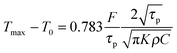 | (2) |
The total fluence (F) absorbed by solvents used is calculated from F = A × (1 − |rf|2)F0, where F0 is the laser fluence before the sample chamber and rf is the reflection coefficient, which is calculated from the cover glass refractive index, n, using the relation  . “A” is the measured absorbance of binary mixtures in the thin sample chamber. The other parameters used in eqn (2) (see S2, ESI†) are density (ρ), thermal conductivity (κ), and heat capacity (C) for binary mixtures that can be calculated from the following set of equations, using pure component physical parameters (Table 1):44–48
| |  | (3) |
In eqn (3) the index j is 2 for binary mixtures, whereas the index i represents the pure component of binary mixtures. The mole fraction (X) is calculated from the volume fraction (φ) and molecular weight (M) and density (ρ). We note that use of such an ideal behaviour is impractical for viscosity, which is dependent on intermolecular interactions. The viscosity of binary mixtures is calculated based on the temperature rise (Tables 2 and 3) using the following equations:49–51| | ln![[thin space (1/6-em)]](https://www.rsc.org/images/entities/char_2009.gif) ηbinarymix = φ1lnη1 + φ2lnη2 + Δlnηexcess ηbinarymix = φ1lnη1 + φ2lnη2 + Δlnηexcess | (4) |
| |  | (5) |
Here Δln(ηexcess) is the excess viscosity due to mixing, which is calculated by using the method developed by Wolf et al.52,53 For each individual alcohol, A, B and C are Vogel’s equation parameters (see S3, ESI†).
Table 1 The used physical parameters of the trapping solvent
| Sample |
Density (ρ) (kg m−3) |
Heat capacity (C) (J kg−1 K−1) |
Thermal conductivity (κ) (W K−1 m−1) |
Absorbance (A) |
|
From ref. 44.
From ref. 45.
From ref. 46.
From ref. 47.
From ref. 48.
|
| H2O |
997a |
4180c |
0.600e |
|
| MeOH |
786b |
2250d |
0.206e |
|
| EtOH |
785b |
2440c |
0.178e |
|
| H2O–EtOH mixture |
990 |
4120 |
0.586 |
0.113 |
| H2O–MeOH mixture |
987 |
4090 |
0.581 |
0.117 |
Table 2 Theoretical and experimental data for a 90:10 (volume-wise) H2O–EtOH mixture
| 1560 nm Power (μW) |
Corner frequency (Hz) |
Fluence (J m−2) |
Theoretical data |
Experimental data |
|
T
max − T0 (K) |
Viscosity (Pa s) × 10−3 |
Corrected ΔTtheo |
Corrected viscosity (Pa s) × 10−3 |
Temperature rise (K) |
Viscosity (Pa s) × 10−3 |
| 0 |
83 |
0 |
0 |
1.60 |
0 |
1.60 |
0 |
1.60 |
| 209 |
88 |
0.0672 |
7.6 |
1.32 |
5.5 |
1.35 |
2.2 |
1.51 |
| 363 |
96 |
0.1167 |
13.2 |
1.23 |
9.6 |
1.29 |
6.1 |
1.38 |
| 420 |
110 |
0.1351 |
15.3 |
1.19 |
11.1 |
1.25 |
12.5 |
1.20 |
| 630 |
119 |
0.2026 |
22.9 |
1.10 |
16.6 |
1.18 |
16.2 |
1.11 |
| 830 |
133 |
0.2669 |
30.2 |
1.02 |
21.9 |
1.10 |
21.5 |
0.99 |
Table 3 Theoretical and experimental data for a 90:10 (volume-wise) H2O–MeOH mixture
| 1560 nm Power (μW) |
Corner frequency (Hz) |
Fluence (J m−2) |
Theoretical data |
Experimental data |
|
T
max − T0 (K) |
Viscosity (Pa s) × 10−3 |
Corrected ΔTtheo |
Corrected viscosity (Pa s) × 10−3 |
Temperature rise (K) |
Viscosity (Pa s) × 10−3 |
| 0 |
106 |
0 |
0 |
1.30 |
0 |
1.30 |
0 |
1.30 |
| 170 |
116 |
0.0547 |
6.5 |
1.14 |
4.8 |
1.18 |
3.9 |
1.19 |
| 266 |
122 |
0.0855 |
10.1 |
1.10 |
7.4 |
1.14 |
6.2 |
1.13 |
| 363 |
129 |
0.1167 |
13.8 |
1.05 |
10.2 |
1.10 |
8.8 |
1.07 |
| 460 |
137 |
0.1479 |
17.5 |
1.00 |
12.9 |
1.06 |
11.5 |
1.01 |
| 630 |
143 |
0.2026 |
23.9 |
0.93 |
17.6 |
1.00 |
14.0 |
0.96 |
| 763 |
150 |
0.2454 |
29.0 |
0.88 |
21.4 |
0.96 |
16.1 |
0.92 |
3.2 Experimental section
We have used a pulsed laser at 780 nm with 7 mW of average power to trap the polystyrene bead of 500 nm mean radius. The solvent media used are H2O–EtOH and H2O–MeOH mixtures. In both the cases, a volume ratio of 90:10 is used. The trapping laser can be considered non-invasive due to very low absorption coefficients of the solvents used.7 Simultaneously, we also irradiated our trapped volume by a 1560 nm IR laser where binary solvents have high absorption coefficients resulting in local heating around the trapped particle. The beam waist spot size of the trapping laser is 680 nm and that of the heating laser is 1360 nm whereas the effective heating beam radius at the trapping plane is out of the Rayleigh range54 (πω02/λ = 931 nm) as the separation is 1.6 μm (see Theoretical section for details). Due to the temperature rise, the trapped 500 nm mean radius particle will show a different behaviour, which is reflected in its “Hot Brownian motion”.55–57 We measure the temperature change between the polystyrene bead surface and the surrounding liquid layer (through the corner frequency shift) to indicate that thermal flow exists, and the bead displacement due to this flow is coupled with that of a regular confined Brownian motion. We only correlate the measured displacement of the confined Brownian motion as long as our temperature change is not very large according to our model. We have thus probed the confined Brownian motion of the polystyrene bead trapped in a harmonic potential58 generated by a Gaussian laser pulse, which can be described by the Langevin equation59| | | mẌ(t) + γẋ(t) + κTSx(t) = ζtherm(t) | (6) |
where m denotes the particle mass, x signifies the time dependent position, γ is the viscous drag coefficient as per Stokes’ law, κTS is the spring constant (or trap stiffness) and ζtherm is the time dependent random force. By solving the above equation, we can fit our experimental one-sided power spectrum. Typically, in the power spectrum, power is measured in the interval f and f + df, which does not distinguish between +f and −f. In such cases, it is possible to define one-sided power spectral density60 (PSD) (see S4, ESI†) by the following Lorentzian:61| |  | (7) |
Here A is a fitting parameter which has information about D, the diffusion coefficient. “A” has the unit V2 s−1. The diffusion coefficient can be evaluated from A using the voltage to position calibration62,63 factor. We have analysed the forward scattered data of the trapped bead that have been collected with a QPD at a sampling rate of 20 kHz for the first 2.5 seconds of trapping. This is to minimize the convection effects. The acquired data of channels X and Y are de-correlated by removing the cross-talk61,64 between them. The processed data are then fitted with eqn (7) to obtain the respective corner frequency within different solvents and at different 1560 nm laser heating powers.
We observed an increasing trend in the corner frequency (fC), which is deduced from the power spectrum (Fig. 2a and b), with an increase in 1560 nm laser power. From our theoretical model (see eqn (2)), we notice that there is a linear relationship between 1560 nm laser power and the corresponding temperature rise. Simultaneously, from eqn (4) and (5), we note that viscosity decreases with an increase in 1560 nm power. Within our experimental range, when the viscosity change with respect to the temperature change lies in the linear regime, we have considered the trap stiffness (κ = 2πfCγ) as a constant parameter. This statement is correct as long as there is a continuous change in viscosity with the heating laser source for a constant-sized trapped particle in the same solvent medium (see S5, ESI†). This has enabled us to measure (Tables 2 and 3) the viscosity change and the temperature rise around the interface of the trapped bead and the surrounding solvent molecules from the formula η·fC = constant.19,65 All our experimental measurements are performed with respect to the room temperature viscosity at the corresponding corner frequency in individual binary solvents when the 1560 nm laser is absent.
 |
| | Fig. 2 Experimentally measured power spectrum (scatter points) and the respective Lorentzian fitted data (solid line) for a 500 nm radius fluorophore coated polystyrene bead in the (a) water–ethanol mixture and (b) water–methanol mixture. | |
Experimentally, we first observe the corner frequency change, which allows us to calculate the viscosity around the trapped bead. From our experimentally measured viscosity, we calculate the temperature rise of the respective binary mixtures (Tables 2 and 3) by rearranging the variables in eqn (5) and solving with MATLAB®. The particle experiencing viscous drag, γ = 6πηr (r = 500 nm), has trap stiffness, κTS, for H2O–EtOH and H2O–MeOH binary mixtures as 0.0078 ± 0.0002 pN nm−1 and 0.0081 ± 0.0002 pN nm−1 respectively. The confidence range of our trap stiffness (see S5, ESI†) results is obtained by the standard deviation of all stiffness measurements at different temperatures. As expected, viscosity changes around the trapped bead with respect to temperature changes are linear (Fig. 3a). Our experimental data in Tables 2 and 3 show that the temperature rise between the theoretical calculation and the experimental measurement deviates with the increase in temperature, which is also true for viscosity. This is due to the fact that besides conduction, convection also plays an important role in heat transfer towards high temperature, since with temperature rise, the focal plane separation changes. The refractive index changes as a result of the diverging optical lens66 formed in solvent media with the increase in temperature at the focal volume. Additionally, due to the high NA objective, there could be a critical angle effect, which could consistently result in an overestimation of our theoretically estimated temperature change. Consequently, the separation of focal points for the two laser wavelengths becomes slightly more, which reduces the temperature at the focal volume around the optical trap and this is reflected in our experimental results. To account for this, we add a correction term to eqn (2) from our earlier study (see S6, ESI†) and generalize it for use in binary mixtures:
| |  | (8) |
Since water is the dominant species in our particular experiments, we can simplify
eqn (8) further as follows:
| |  | (8a) |
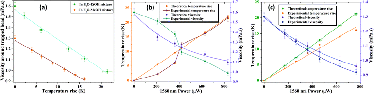 |
| | Fig. 3 (a) Experimental data for viscosity versus temperature rise (scatter plot) around the trapped bead and the corresponding linear fitting (solid line). The comparison of our theoretically corrected data for temperature rise (left side Y axis) and viscosity (right side Y axis) with experimental data in the respective (b) water–ethanol mixture and (c) water–methanol mixture. | |
Here C1 represents pure water while the other parameters are the same as explained in the Theoretical section. In pure water, the theoretical gradient of temperature rise, calculated from eqn (2), is (dT/dP)Theo = 0.034 K μW−1, while the measured experimental gradient of temperature rise is (dT/dP)Exp = 0.024 K μW−1. The correction term introduced is the difference of these two values for binary solvent mixtures in eqn (8a). We plot the corrected theoretical temperature rise and the corresponding viscosity in Fig. 3b and c for H2O–EtOH and H2O–MeOH respectively and compare them to the corresponding experimental data (also presented in Tables 2 and 3). For theoretical calculations, we first estimated the temperature rise (Tmax − T0 (K)) from applied 1560 nm pulse laser fluence using eqn (2), which is converted viaeqn (5) to measure the surrounding viscosity. The corrected ΔTtheo is evaluated from eqn (8a), which is again transformed to measure the corrected viscosity using eqn (5).
It is important to note from Fig. 3b that we observed a very unusual experimental behaviour of temperature rise (ΔT) and viscosity (η) in the H2O–EtOH binary mixture. This is in spite of the fact that the theoretical temperature rise (ΔT) followed a linear increase with 1560 nm laser power, and the viscosity (η) followed the Vogel equation. This unusual behaviour is due to the loss of the individual properties of the constituent liquids in the binary mixtures, which is better explained in terms of non-ideal behaviour of the binary mixture as presented in Fig. 4. Fig. 4a shows the comparative plot of the slope of 1/fC with 1560 nm laser power for water with methanol as well as ethanol. The distinct behaviour of the nature of the trap is evident from the distinct slopes in Fig. 4a for the three pure liquids, i.e., water (−2.95), methanol (−5.71) and ethanol (2.06), which also conform to the trend in the respective viscosities (η) of these pure liquids (ηEtOH > ηH2O > ηMeOH). These numbers are indicative of the fact that the intermolecular forces in pure water and in pure ethanol are more similar as compared to the intermolecular forces in pure methanol. This would mean that in the case of binary mixtures of water with ethanol or methanol, the water–ethanol mixture would overall have more intermolecular force as compared to that of water–methanol. To further ratify our conjecture obtained from Fig. 4a, we plotted the comparative excess heat capacity in Fig. 4b, which shows that for a 10% volume mixture of H2O–MeOH and H2O–EtOH, the excess heat capacity, CEp,mix, of the water–ethanol mixture (6.69 J K−1 mol−1) is higher than that of the water–methanol mixture (1.74 J K−1 mol−1).
 |
| | Fig. 4 (a) Comparative plot of inverse corner frequency versus power of a 1560 nm femtosecond laser with linear fitting (solid line) of water with pure MeOH and pure EtOH. (b) The comparison between excess heat capacity of H2O–MeOH (black line) and H2O–EtOH (red line) binary mixtures at 25 °C. | |
Since excess heat capacity is the measure of deviation from the ideal nature of mixtures, water–ethanol shows a higher deviation from ideal behaviour as compared to water–methanol. This corresponds to our observation from Fig. 3 that the water–methanol mixture follows the expected trend of 1560 nm laser heating while the water–ethanol mixture shows deviation.
The isobaric molar heat capacity of the binary mixture can be expressed by eqn (9) and (10). Thus, the excess heat capacity can be calculated by using eqn (11):67
| |  | (9) |
| | | Cp,m,mix = XC1Cp,C1 + XC2Cp,C2 + CEp,mix | (10) |
| | 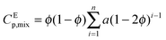 | (11) |
where C2 represents the second component of the binary mixture with water,
H is the enthalpy,
φ is the volume fraction of water and the “
a” value is used from
ref. 67.
Thus, our experimental results follow our theoretical framework that we have developed for the measurement of sub-micron volume temperatures as well as viscosity. For trapping polystyrene beads, individual solvents like H2O, MeOH and EtOH are good solvents and they are also miscible among each other.68 We report our findings for a 90:10 volume mixture of H2O–EtOH and H2O–MeOH. When the volume of alcohol in water–alcohol binary mixtures increases beyond 10%, the viscosity of water-alcohol mixture increases rapidly until an equal volume mixture is reached.69 Higher viscosity results in lower corner frequency. Thus, the corner frequency shift due to the temperature rise will be small, which will decrease the experimental signal to noise ratio.
4. Conclusions
In this work, based on a non-invasive 780 nm femtosecond optical trap, we have demonstrated the control and measurement of direct in situ temperature at the solid–liquid interface, induced by a co-propagating 1560 nm pulsed laser. The viscosity as well as temperature around the trapped bead has been measured from the changes in corner frequency values. These measurements show that the thermal energy of solvents is transformed into the kinetic energy of the trapped bead. Correspondingly, we have developed a theoretical model that can explain these experimental results. Last but not the least, we were also able to probe the intermolecular interaction between two closely behaving solvent molecules.
Acknowledgements
We thank the Wellcome Trust Senior Research Fellowship (UK), the ISRO Science Technology Cell and DST, Govt. of India, for funding research presented here. DM thanks UGC, India, for the graduate fellowship. We thank D. Roy for useful discussions. We also thank Mrs S. Goswami for language editing of this article.
References
- A. Ashkin, J. M. Dziedzic, J. E. Bjorkhom and S. Chu, Opt. Lett., 1986, 11, 288–290 CrossRef CAS PubMed.
-
A. Ashkin, Optical Trapping and Manipulation of Neutral Particles Using Lasers: A Reprint Volume with Commentaries, World Scientific, 2006 Search PubMed.
- Q. Xing, F. Mao, L. Chai and Q. Wang, Opt. Laser Technol., 2004, 36, 635–639 CrossRef.
- B. Agate, C. T. A. Brown, W. Sibbett and K. Dholakia, Opt. Express, 2004, 12, 3011–3017 CAS.
- A. K. De, D. Roy, A. Dutta and D. Goswami, Appl. Opt., 2009, 48, G33–G37 CrossRef PubMed.
- D. Roy, A. K. De and D. Goswami, Appl. Opt., 2015, 54, 7002–7006 CrossRef PubMed.
- A. Schönle and S. W. Hell, Opt. Lett., 1998, 23, 325–327 CrossRef.
- P. Kumar and D. Goswami, J. Phys. Chem. C, 2014, 118, 14852–14859 CAS.
- D. Mondal and D. Goswami, Biomed. Opt. Express, 2015, 6, 3190–3196 CrossRef PubMed.
- D. Mondal and D. Goswami, J. Nanophotonics, 2016, 10, 026013 CrossRef.
- A. Ashkin and J. M. Dziedzic, Science, 1987, 235, 1517–1520 CAS.
- S. M. Block, D. F. Blair and H. C. Berg, Nature, 1989, 338, 514–518 CrossRef CAS PubMed.
- A. Ashkin and J. M. Dziedzic, Proc. Natl. Acad. Sci. U. S. A., 1989, 86, 7914–7918 CrossRef CAS.
- A. Ashkin, J. M. Dziedzic and T. Yamane, Nature, 1987, 330, 769–771 CrossRef CAS PubMed.
-
G. Herzberg, Infrared and Raman Spectra, D. Van Nostrand: Princeton, 1945 Search PubMed.
- C. L. Braun and S. N. Smirnov, J. Chem. Educ., 1993, 70, 612–614 CrossRef CAS.
- A. I. Bishop, T. A. Nieminen, N. R. Heckenberg and H. Rubinsztein-Dunlop, Phys. Rev. Lett., 2004, 92, 198104 CrossRef PubMed.
- A. Pommella, V. Preziosi, S. Caserta, J. M. Cooper, S. Guido and M. Tassieri, Langmuir, 2013, 29, 9224–9230 CrossRef CAS PubMed.
- M. Tassieri, F. D. Giudice, E. J. Robertson, N. Jain, B. Fries, R. Wilson, A. Glidle, F. Greco, P. A. Netti, P. L. Maffettone, T. Bicanic and J. M. Cooper, Sci. Rep., 2015, 5, 8831 CrossRef CAS PubMed.
- Y. M. Rhee and V. S. Pande, J. Phys. Chem. B, 2008, 112, 6221–6227 CrossRef CAS PubMed.
- D. de Sancho, A. Sirur and R. B. Best, Nat. Commun., 2014, 5, 4307 CAS.
- M. Guoa, Y. Xub and M. Gruebelea, Proc. Natl. Acad. Sci. U. S. A., 2012, 109, 17863–17867 CrossRef PubMed.
- M. Karplus and J. A. Mccammon, Nat. Struct. Mol. Biol., 2002, 9, 646–652 CAS.
- R. M. Daniel, M. E. Peterson, M. J. Danson, N. C. Price, S. M. Kelly, C. R. Monk, C. S. Weinberg, M. L. Oudshoorn and C. K. Lee, Biochem. J., 2010, 425, 353–360 CrossRef CAS PubMed.
- M. L. Begasse, M. Leaver, F. Vazquez, S. W. Grill and A. A. Hyman, Cell Rep., 2015, 10, 647–653 CrossRef CAS PubMed.
- G. E. Uhlenbeck and L. S. Ornstein, Phys. Rev., 1930, 36, 823–841 CrossRef CAS.
- M. C. Wang and G. E. Uhlenbeck, Rev. Mod. Phys., 1945, 17, 323–342 CrossRef.
- A. Einstein, Ann. Phys., 1905, 322, 549–560 CrossRef.
-
F. Reif, Fundamentals of statistical and thermal physics, McGraw-Hill, Sydney, 1965 Search PubMed.
- T. G. Mason, K. Ganesan, J. H. van Zanten, D. Wirtz and S. C. Kuo, Phys. Rev. Lett., 1997, 97, 3282–3285 CrossRef.
- F. C. MacKintosha and C. F. Schmidt, Curr. Opin. Colloid Interface Sci., 1999, 4, 300–307 CrossRef.
- M. Atakhorrami, J. I. Sulkowska, K. M. Addas, G. H. Koenderink, J. X. Tang, A. J. Levine, F. C. MacKintosh and C. F. Schmidt, Phys. Rev. E: Stat., Nonlinear, Soft Matter Phys., 2006, 73, 061501 CrossRef CAS PubMed.
- A. Yao, M. Tassieri, M. Padgett and J. Cooper, Lab Chip, 2009, 9, 2568–2575 RSC.
- T. Kalwarczyk, N. Zie-bacz, A. Bielejewska, E. Zaboklicka, K. Koynov, J. Szymanski, A. Wilk, A. Patkowski, J. Gapinski, H.-J. Butt and R. Hozyst, Nano Lett., 2011, 11, 2157–2163 CrossRef CAS PubMed.
- G. Charras and E. Sahai, Nat. Rev. Mol. Cell Biol., 2014, 15, 813–824 CrossRef CAS PubMed.
- Y. Pang and R. Gordon, Nano Lett., 2012, 12, 402–406 CrossRef CAS PubMed.
- D. Mondal and D. Goswami, SPIE Proc., 2015, 9548, 95481N CrossRef.
- P. Kumar, A. Khan and D. Goswami, Chem. Phys., 2014, 441, 5–10 CrossRef CAS.
-
J. H. Lienhard IV and J. H. Lienhard V, A Heat Transfer Textbook, Phlogiston Press, Cambridge, Massachusetts, USA, 3rd edn, 2004 Search PubMed.
- Y. Liu, G. J. Sonek, M. W. Berns and B. J. Tromberg, Biophys. J., 1996, 71, 2158–2167 CrossRef CAS PubMed.
-
H. S. M. Coxeter and S. L. Greitzer, Geometry Revisited, The Mathematical Association of America, Washington, DC, 1967 Search PubMed.
-
http://www.olympus-ims.com/en/microscope/terms/luminous_flux/(accessed 14 July, 2016).
-
X. E. Lin, in Proceedings of the 1999 Particle Accelerator Conference, (IEEE, 1999), 1429–1431.
- T. A. Scott, J. Phys. Chem., 1946, 50, 406–412 CrossRef CAS PubMed.
- J. Ortega, J. Chem. Eng. Data, 1982, 27, 312–317 CrossRef CAS.
- J.-P. E. Grolier, Fluid Phase Equilibrium, 1981, 6, 283–287 CrossRef CAS.
- G. C. Benson, P. J. D’Arcy and O. K. Kiyohara, J. Solution Chem., 1980, 9, 931–938 CrossRef CAS.
- J. D. Raal and R. L. Rijsdijk, J. Chem. Eng. Data, 1981, 26, 351–359 CrossRef CAS.
-
T. Al-Shemmeri, Engineering Fluid Mechnanics, Ventus Publishing ApS, 2012 Search PubMed.
- Dartmund Data Bank (DDB), http://ddbonline.ddbst.de/VogelCalculation/VogelCalculationCGI.exe.
- J. Kendall and K. P. Monroe, J. Am. Chem. Soc., 1917, 39, 1787–1802 CrossRef CAS.
- M. Schnell and B. A. Wolf, J. Rheol., 2000, 44, 617–628 CrossRef CAS.
- R. Mertsch and B. A. Wolf, Ber. Bunsenges. Phys. Chem., 1994, 98, 1275–1280 CrossRef CAS.
-
S. N. Damask, Polarization Optics in Telecommunications, Springer-Verlag, New York, 2005 Search PubMed.
- R. Radünz, D. Rings, K. Kroy and F. Cichos, J. Phys. Chem. A, 2009, 115, 1674–1677 CrossRef PubMed.
- D. Rings, R. Schachoff, M. Selmke, F. Cichos and K. Kroy, Phys. Rev. Lett., 2010, 105, 090604 CrossRef PubMed.
- L. Joly, S. Merabia and J.-L. Barrat, Europhys. Lett., 2011, 94, 50007 CrossRef.
- A. C. Richardson, S. N. S. Reihani and L. B. Oddershede, Opt. Express, 2008, 16, 15709–15717 CrossRef CAS PubMed.
-
R. Kubo, M. Toda and N. Hashitsume, Statistical Physics, Springer, Heidelberg, 1985, vol. 2 Search PubMed.
-
W. H. Press, B. P. Flannery, S. A. Teukolsky and W. T. Vetterling, Numerical Recipes. The Art of Scientific Computing, Cambridge University Press, Cambridge, ch. 12.0, 1998 Search PubMed.
- K. Berg-Sørensen and H. Flyvbjerg, Rev. Sci. Instrum., 2004, 75, 594–612 CrossRef.
- G. Pesce, A. Sasso and S. Fusco, Rev. Sci. Instrum., 2005, 76, 115105 CrossRef.
- S. F. Tolić-Nørrelykkea, E. Schäffer, J. Howard, F. S. Pavone, F. Jülicher and H. Flyvbjerg, Rev. Sci. Instrum., 2006, 77, 103101 CrossRef.
- I.-M. Tolić-Nørrelykkea, K. Berg-Sørensen and H. Flyvbjerg, Comput. Phys. Commun., 2004, 159, 225–240 CrossRef.
- H. Mao, J. R. Arias-Gonzalez, S. B. Smith, I. Tinoco, Jr. and C. Bustamante, Biophys. J., 2005, 89, 1308–1316 CrossRef CAS PubMed.
- A. Marcano, C. Loper and N. Melikechi, J. Opt. Soc. Am. B, 2002, 19, 119–124 CrossRef CAS.
- G. C. Benson, P. J. D'Arcy and O. Kiyohara, J. Solution Chem., 1980, 9, 931–938 CrossRef CAS.
- D. Mukherji, C. M. Marques and K. Kremer, Nat. Commun., 2014, 5, 4882 CrossRef PubMed.
- E. J. W. Wensink, A. C. Hoffmann, P. J. van Maaren and D. van der Spoel, J. Chem. Phys., 2003, 119, 7308–7317 CrossRef CAS.
Footnote |
| † Electronic supplementary information (ESI) available. See DOI: 10.1039/c6cp03093a |
|
| This journal is © the Owner Societies 2016 |
Click here to see how this site uses Cookies. View our privacy policy here. 
 Open Access Article
 This Open Access Article is licensed under a Creative Commons Attribution-Non Commercial 3.0 Unported Licence
 *ab
*ab


 . “A” is the measured absorbance of binary mixtures in the thin sample chamber. The other parameters used in eqn (2) (see S2, ESI†) are density (ρ), thermal conductivity (κ), and heat capacity (C) for binary mixtures that can be calculated from the following set of equations, using pure component physical parameters (Table 1):44–48