Multiple superhyperfine fields in a {DyFe₂Dy} coordination cluster revealed using bulk susceptibility and ⁵⁷Fe Mössbauer studies

Abstract

A [DyFe^III₂Dy(μ₃-OH)₂(pmide)₂(p-Me-PhCO₂)₆] coordination cluster, where pmideH₂ = N-(2-pyridylmethyl)iminodiethanol, has been synthesized and the magnetic properties studied. The dc magnetic measurements reveal dominant antiferromagnetic interactions between the metal centres. The ac measurements reveal zero-field quantum tunnelling of the magnetisation (QTM) which can be understood, but not adequately modelled, in terms of at least three relaxation processes when appropriate static (dc) fields are applied. To investigate this further, ⁵⁷Fe Mössbauer spectroscopy was used and well-resolved nuclear hyperfine structures could be observed, showing that on the Mössbauer time scale, without applied field or else with very small applied fields, the iron nuclei experience three or more superhyperfine fields arising from the slow magnetisation reversal of the strongly polarized fields of the Dy^III ions.

---

Introduction

Magnetic bistability in molecules has been extensively studied and analysed in recent years in the context of the so-called Single Molecule Magnets (SMMs). These show slow relaxation of their magnetisation as the result of an inherent energy barrier to spin inversion and this can be estimated from an analysis of the relaxation processes, in the most favourable cases using an Arrhenius law to estimate an effective barrier, U_eff, which suggests a barrier height for spin inversion of the ground spin state via all the intervening microstates. Studies on superparamagnetic nanoparticles rely more on the concept of a blocking temperature which defines the point below which slow relaxation can be observed and this is dependent on timescale factors for the chosen measurement method. Whereas ⁵⁷Fe Mössbauer spectroscopy (MS) has been the method of choice for investigating superparamagnetic iron oxide nanoparticles,¹ the simple fact that few groups working on SMMs have incorporated iron into their systems means that Mössbauer spectroscopy has rarely been used to provide added insights into the relaxation processes of SMMs.

An appealing means to increase U_eff is to incorporate 4f (lanthanide) ions into SMM systems since these possess both high spins and large magnetic anisotropies.² Although this can lead to compounds with U_eff barriers of up to 800 K for pure lanthanide systems,³ the fact that a barrier is there does not mean that it cannot be circumvented and various tunnelling and relaxation processes provide easier routes to the “other side” than having to “go over the top”.

Although the approach of using combinations of highly anisotropic lanthanide and paramagnetic transition metals to give 3d/4f systems often leads to lower U_eff values, the fact that Quantum Tunnelling of the Magnetisation (QTM) effects can be suppressed still leads to enhanced SMM properties with some examples showing higher blocking temperatures and improved static field properties, i.e. without the need to apply fields to suppress QTM. Such 3d–4f blends can lead to the observation of exotic magnetic effects such as coexistence of two mechanisms for blocking of magnetisation – single-ion and exchange-based.⁴

Such 3d–4f systems have mostly been investigated using standard bulk susceptibility, including ac studies, as an experimental method to quantify the relaxation processes and this approach is clearly not sufficient. In order to understand the details of the relaxation processes single crystal studies and/or theoretical studies can be of help.^5,6 In the special case where the 3d ion is Feⁿ⁺ we have shown how this can act as a sensor for the local anisotropy exerted by the 4f ions using a Mössbauer spectroscopy approach. This makes it possible to sense the local coupling regimes between pairs of metal centres at a microscopic level,^7–9 as shown for a Dy/Tb system.⁷ This means of going beyond standard magnetic susceptibility techniques provides an important experimental method to assist theoreticians in their quest to improve their descriptions of these challenging systems, which involve highly anisotropic magnetic centers showing significant spin–orbit coupling. For these purposes we chose to probe the magnetism and Mössbauer spectroscopy of a tetranuclear compound [DyFe^III₂Dy(μ₃-OH)₂(pmide)₂(p-Me-PhCO₂)₆] (1), where pmideH₂ = N-(2-pyridylmethyl)iminodiethanol. In order to extract the iron and dysprosium magnetic contributions the yttrium and aluminium isostructural analogues were also synthesised, namely [YFe^III₂Y(μ₃-OH)₂(pmide)₂(p-Me-PhCO₂)₆] (2) and [DyAl₂Dy(μ₃-OH)₂(pmide)₂(p-Me-PhCO₂)₆] (3).

Experimental section

General information

All chemicals and solvents used for synthesis were obtained from commercial sources and used as received without further purification. All reactions were carried out under aerobic conditions. N-(2-pyridylmethyl)iminodiethanol was prepared according to the literature procedure.¹⁰ The elemental analyses (C, H, and N) were carried out using an ElementarVario EL analyzer. Fourier transform IR spectra (4000 to 400 cm⁻¹) were measured on a Perkin-Elmer Spectrum GX spectrometer with samples prepared as KBr discs.

Synthesis of [Fe^III₂Dy₂(μ₃-OH)₂(pmide)₂(p-Me-PhCO₂)₆]·2MeCN (1)

N-(2-pyridylmethyl)iminodiethanol (100 mg, 0.5 mmol) in MeCN (5 ml) was added to a solution of FeCl₂·4H₂O (50 mg, 0.25 mmol), DyCl₃·6H₂O (94 mg, 0.25 mmol) and 4-methylbenzoic acid (144 mg, 1 mmol) in MeCN (20 ml) and MeOH (5 ml). After 10 min of stirring, Et₃N (0.42 ml, 3 mmol) was added, leaving the solution stirring for a further 0.5 h. The final solution was filtered and left undisturbed. After leaving overnight pale yellow single crystals suitable for X-ray analysis were collected and air dried. Yield: 61% (187.5 mg, based on 4-methylbenzoic acid). Anal. calcd (found) % for Fe₂Dy₂C₆₈H₇₂N₄O₁₈·2MeCN·MeOH·3.35H₂O: C, 47.53 (47.29); H, 4.85 (4.61); N, 4.56 (4.51). Selected IR data (KBr, cm⁻¹) for 1: 3503 (br), 3058 (w), 2975 (w), 2854 (m), 1593 (s), 1541 (s), 1099 (s), 906 (s), 722 (s), 672 (s), 593 (s). Note that this compound can also be prepared starting from Fe^III salts.

Synthesis of [Fe^III₂Y₂(μ₃-OH)₂(pmide)₂(p-Me-PhCO₂)₆]·2MeCN (2)

Compound 2 was synthesised in a similar manner as for 1 but with YCl₃·6H₂O in place of DyCl₃·6H₂O Yield: 58% (152.8 mg, based on 4-methylbenzoic acid). Anal. calcd (found) % for Fe₂Y₂C₆₈H₇₂N₄O₁₈·MeCN: C, 53.15 (53.05); H, 4.91 (4.80); N, 4.43 (4.29). The IR is similar to that of 1.

Synthesis of [Al₂Dy₂(μ₃-OH)₂(pmide)₂(p-Me-PhCO₂)₆]·2MeCN(3)

Compound 3 was synthesised using a similar method as for 1 with AlCl₃·6H₂O in place of FeCl₂·4H₂O Yield: 72% (203.3 mg, based on 4-methylbenzoic acid). Anal. calcd (found) % for Al₂Dy₂C₆₈H₇₂N₄O₁₈·MeCN: C, 50.85 (50.92); H, 4.57 (4.60); N, 4.24 (3.91). Selected IR data (KBr, cm⁻¹) for 3: 3497 (br), 3055 (w), 2976 (w), 2854 (m), 1591 (s), 1543 (s), 1096 (s), 905 (s), 723 (s), 675 (s), 591 (s).

Mössbauer spectroscopy

Mössbauer Spectra were acquired in transmission geometry with a conventional spectrometer incorporating an Oxford Instruments Mössbauer-Spectromag 4000 Cryostat, equipped with a ⁵⁷Co source (3.7 GBq) in a rhodium matrix in the constant-acceleration mode. Isomer shifts are given relative to α-Fe at 300 K.

Magnetic measurements

The magnetic susceptibility measurements were obtained using a Quantum Design SQUID magnetometer MPMS-XL in the temperature range 1.8–300 K. Measurements were performed on polycrystalline samples restrained in eicosane and contained in sealed plastic bags. Magnetisation isotherms were collected at 2, 3, 5 K between 0 and 7 T. Alternating current (ac) susceptibility measurements were performed with an oscillating field of 3 Oe and ac frequencies ranging from 0.05 to 1500 Hz. The magnetic data were corrected for the sample holder and the diamagnetic contribution.

X-ray analysis

The X-ray data were collected on an Oxford Diffraction Supernova E diffractometer, using Mo-K_α radiation (λ = 0.71073 Å) from a microfocus source. Structures were solved by dual-space direct methods using SHELXT^11a and refined against F_o² using SHELXL-2014^11b with anisotropic displacement parameters for all non-hydrogen atoms. Organic hydrogen atoms were placed in calculated positions; the coordinates of H(1) were refined. Crystallographic data for the structures of 1 and 3 have been deposited with the Cambridge Crystallographic Data Centre as supplementary publications CCDC 1428524 and 1428525. Copies of the data can be obtained from: http://summary.ccdc.cam.ac.uk/structure-summary-form.

Results and discussion

Structural description

The three compounds are isostructural and we describe here compound 1 in detail. The crystal parameters of the three compounds are summarised in Table 1. Compound 1 (Fig. 1) crystallises in the monoclinic space group C2/c and has a similar core motif to the previously reported Fe^III₂Dy₂ coordination clusters formed from the reaction of triethanolamine derivatives and (substituted) benzoate co-ligands, in which a central Fe^III₂ unit is flanked by two Dy centres.^8,9

Table 1 Crystallographic data and structural refinements for 1–3

Compound	1	2	3
Formula	C72H78Dy2Fe2N6O18	C72H78Y2Fe2N6O18	C72H78Al2Dy2N6O18
M r [g mol^−1]	1752.10		1694.36
Colour	Pale-yellow	Pale-yellow	Colourless
Crystal system	Monoclinic	Monoclinic	Monoclinic
Space group	C2/c	C2/c	C2/c
T [K]	180	180	150
a [Å]	28.4714(5)	28.4072	27.6565(9)
b [Å]	10.5419(2)	10.6721	10.6992(3)
c [Å]	24.4309 (5)	24.6303	24.5174(7)
α [°]	90	90	90
β [°]	94.949(2)	97.243	94.143(3)
γ [°]	90	90	90
V [Å]	7305.4(2)	7143.3	7235.8(4)
Z	4	4	4
D x [g cm^−3]	1.593		1.555
μ [mm^−1]	2.48		2.15
F(000)	3520		3416
Reflns collected	44 580		38 808
Unique data	9370		8189
R int	0.040		0.050
Data with I > 2σ(I)	8445		7358
Parameters/restraints	458/1		458/0
S on F^2	1.12		1.06
R 1 [I > 2σ(I)]	0.029		0.026
wR2 (all data)	0.060		0.058
Largest diff peak/hole [e Å^−3]	+1.00/−0.59		+0.73/−0.55
CCDC	1428524		1428525

---

Fig. 1 The ligand (H₂pmide) used in this work (left) and molecular structure of compound [DyFe^III₂Dy(μ₃-OH)₂(pmide)₂(p-Me-PhCO₂)₆] (1) (right). Organic H atoms are omitted for clarity. Dy violet; Fe green; O red; N blue; C black, H white.

The compound is essentially isostructural to the previously reported Fe₂Dy₂ compounds prepared with the H₃tea (triethanolamine) ligand.^8,9 As shown in Fig. 1, in compound 1 the chelating alcohol arm of the triethanolamine ligand attached to the Dy centres is substituted by a pyridine containing fragment, which affects the local environments of these metal ions. The two Fe^III ions are six coordinate with octahedral geometries and an average Fe–O bond length of 2.001 Å. The two Dy^III ions are nine coordinate with monocapped square antiprismatic geometries with an average Dy–O/N bond length of 2.441 Å. The Fe⋯Fe distance is 3.211(0) Å and the intramolecular Dy⋯Dy distance is 6.101(1) Å. The closest intermolecular Dy⋯Dy distance is 7.951(1) Å. Selected bond lengths (Å) and angles of compounds 1 and 3 are summarised in Table 2.

Table 2 Selected bond lengths (Å) and angles of compounds 1(Fe₂Dy₂) and 3(Al₂Dy₂)

Compounds	1 (M = Fe^III)	3 (M = Al^III)
Dy1–O2	2.3215(17)	2.3200(15)
Dy1–O3	2.3416(16)	2.3308(16)
Dy1–O1	2.3990(17)	2.4214(16)
Dy1–O8	2.4285(18)	2.4371(17)
Dy1–O7	2.4332(17)	2.4046(16)
Dy1–O9	2.4388(17)	2.4538(16)
Dy1–O5	2.4434(17)	2.4212(16)
Dy1–N2	2.566(2)	2.5640(19)
Dy1–N1	2.618(2)	2.602(2)
M1–O3^i	1.9676(17)	1.8668(17)
M1–O2	1.9738(17)	1.8701(17)
M1–O4	1.9944(17)	1.8875(17)
M1–O6^i	2.0058(17)	1.8977(17)
M1–O1^i	2.0548(16)	1.9347(17)
M1–O1	2.0584(17)	1.9496(17)
O1–M1^i	2.0548(16)	1.9346(17)
M1^i–O1–M1	102.65(7)	102.27(8)
M1^i–O1–Dy1	101.28(7)	101.44(7)
M1–O1–Dy1	100.90(6)	100.85(7)
M1–O2–Dy1	106.32(7)	107.29(7)
M1^i–O3–Dy1	106.07(7)	106.90(7)
M1–M1^i	3.211(0)	3.024(1)
M1–Dy1	3.444(1)	3.383(1)
M1^i—Dy1	3.450(1)	3.386(1)
Dy–Dyintra	6.101(1)	6.055(1)
Dy–Dyinter	7.951(1)	8.093(2)
Symmetry code:	(i) −x + 1/2, −y + 3/2, −z + 1.	(i) −x + 1/2, −y + 3/2, −z + 1.

---

Static magnetic properties

Direct-current (dc) magnetic susceptibility studies of 1 were performed under an applied magnetic field of 300 Oe in the 300–1.8 K temperature range (Fig. 2). The value of χT at 300 K of 35.46 cm³ K mol⁻¹ is slightly lower than the expected value of 36.84 cm³ K mol⁻¹ for two high-spin Fe^III ions (S = 5/2, g = 2, and C = 4.37 cm³ K mol⁻¹) and two Dy^III ions with S = 5/2, L = 5, ⁶H_15/2, g = 4/3 and C = 14.17 cm³ K mol⁻¹.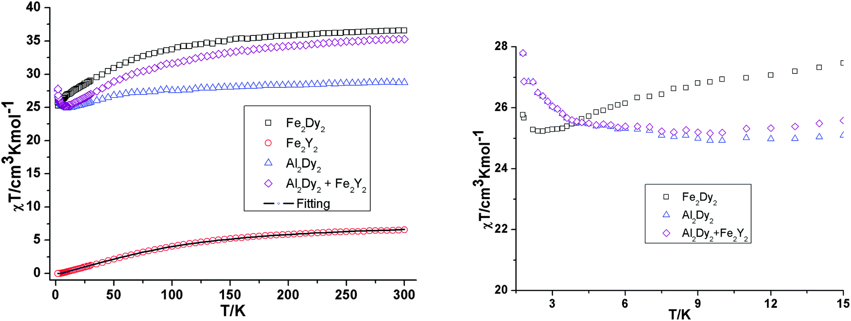

Fig. 2 Temperature dependence (left) of the χT product at 300 Oe for 1, Fe₂Dy₂, 2, Fe₂Y₂ (the solid line is the best fit to the experimental data for 2) and 3, Al₂Dy₂. The comparison curves (right) of Fe₂Dy₂ and Al₂Dy₂ + Fe₂Y₂ along with the curve for 3, Al₂Dy₂ enlarged in the region below 15 K.

There is a steady decrease of the χT product on decreasing the temperature from 300 to 100 K, a more rapid decrease from 100 to 2.5 K, reaching a value of 25.00 cm³ K mol⁻¹, suggesting that antiferromagnetic interactions between paramagnetic centres are present in this molecule. The last minor increase of χT to 25.80 cm³ K mol⁻¹ below 2.5 K is due to weak ferromagnetic interactions. The thermal depopulation of the Dy^III excited states, the sublevels of the ⁶H_15/2 state,¹² is also partially responsible for the continuous decrease of χT below 100 K. As in all reported similar Fe₂Ln₂ compounds,^8,9,13 the interaction between Fe–Fe in complex 1 is antiferromagnetic with an S = 0 ground state. This was proved by the fit of the susceptibility data using the PHI program¹⁴ (Fig. 2) of the compound [YFe^III₂Y(μ₃-OH)₂(pmide)₂(p-CH₃-C₆H₅COO)₆] (2). The fit results are J = −7.0 cm⁻¹ and g = 1.95. The presence of ferromagnetic interactions in compound 1 at low temperature was supported by magnetic studies on the aluminium analogue [DyAl₂Dy(μ₃-OH)₂(pmide)₂(p-CH₃-C₆H₅COO)₆] (3). For compound 3, χT decreases slowly on cooling down to about 15 K, below which it increases to 28.03 cm³ K mol⁻¹ at 1.8 K (Fig. 2) and it is consistent with a weak ferromagnetic Dy⋯Dy interaction also observed for reported {Mg₂Dy₂} and {Dy₂} systems.¹⁵ In order to probe the antiferromagnetic Fe⋯Dy interaction in compound 1, the χT vs. T curves for Fe₂Dy₂, Al₂Dy₂ and Fe₂Y₂ can be compared (Fig. 2). We model the Fe₂Dy₂ data by addition of the curves for Fe₂Y₂ and Al₂Dy₂ which effectively ‘deletes’ the contribution of the Fe⋯Dy interaction. As shown in Fig. 2 (right) the curves corresponding to Al₂Dy₂ and Fe₂Y₂ + Al₂Dy₂ have very similar χT values which essentially coincide at low temperature.

The field dependence of the magnetisation of 1 was performed at fields ranging from 0 to 7 T at 2, 4 and 5 K (Fig. 3). It shows a relatively rapid increase of magnetisation below 1 T. At higher fields, M increases linearly without clear saturation to ultimately reach 11.90 μ_B (H = 7 T, at 2 K). Such behaviour is characteristic for systems dominated by high magnetic anisotropy and through application of an external magnetic field the low-lying excited states are progressively populated.¹³ The field dependences of the magnetisation of 2 and 3 (Fig. 3) show a behaviour typically observed in the antiferromagnetically coupled {Fe^III₂}^8,9,13 and weakly coupled {Dy₂}¹⁵ molecular clusters in polycrystalline form, respectively.

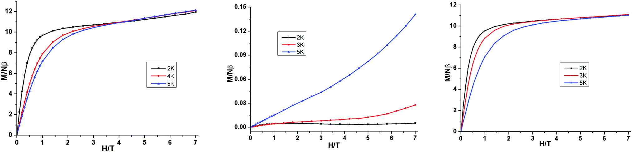Fig. 3 Magnetisation (M) vs. applied field (H) at different temperatures for 1, Fe₂Dy₂, (left); 2, Fe₂Y₂ (middle) and 3, Al₂Dy₂ (right).

Dynamic magnetic properties

{Fe₂Dy₂} (1). In order to probe potential slow magnetisation relaxation, ac magnetic measurements were carried out. For 1, under zero applied dc field, only one relaxation process seems to operate within the frequency window of our measurements (0–1500 Hz) (Fig. 4). After a quick screening at different dc fields (0–3000 Oe) (Fig. 4) an optimum dc field (1000 Oe) was found, at which the minimum of the characteristic frequency was observed and by applying this dc field full peaks in the temperature and frequency dependent out of phase (χ′′) susceptibility measurements were observed (Fig. 5). The presence of peaks that shift to lower frequency as the temperature decreases is indicative of slow magnetisation relaxation. The anisotropic energy barrier was found by fitting using the Arrhenius equation, τ = τ₀e^U_eff/kT, giving U_eff = 16.2 K (11.2 cm⁻¹) (τ₀ = 2.6 × 10⁻⁶ s) (Fig. 6).

Fig. 4 Frequency dependence of the in-phase and out-of-phase components of the ac magnetic susceptibility for 1 (Fe₂Dy₂) at 2 K under different dc fields (0–3000 Oe) (fast screening).

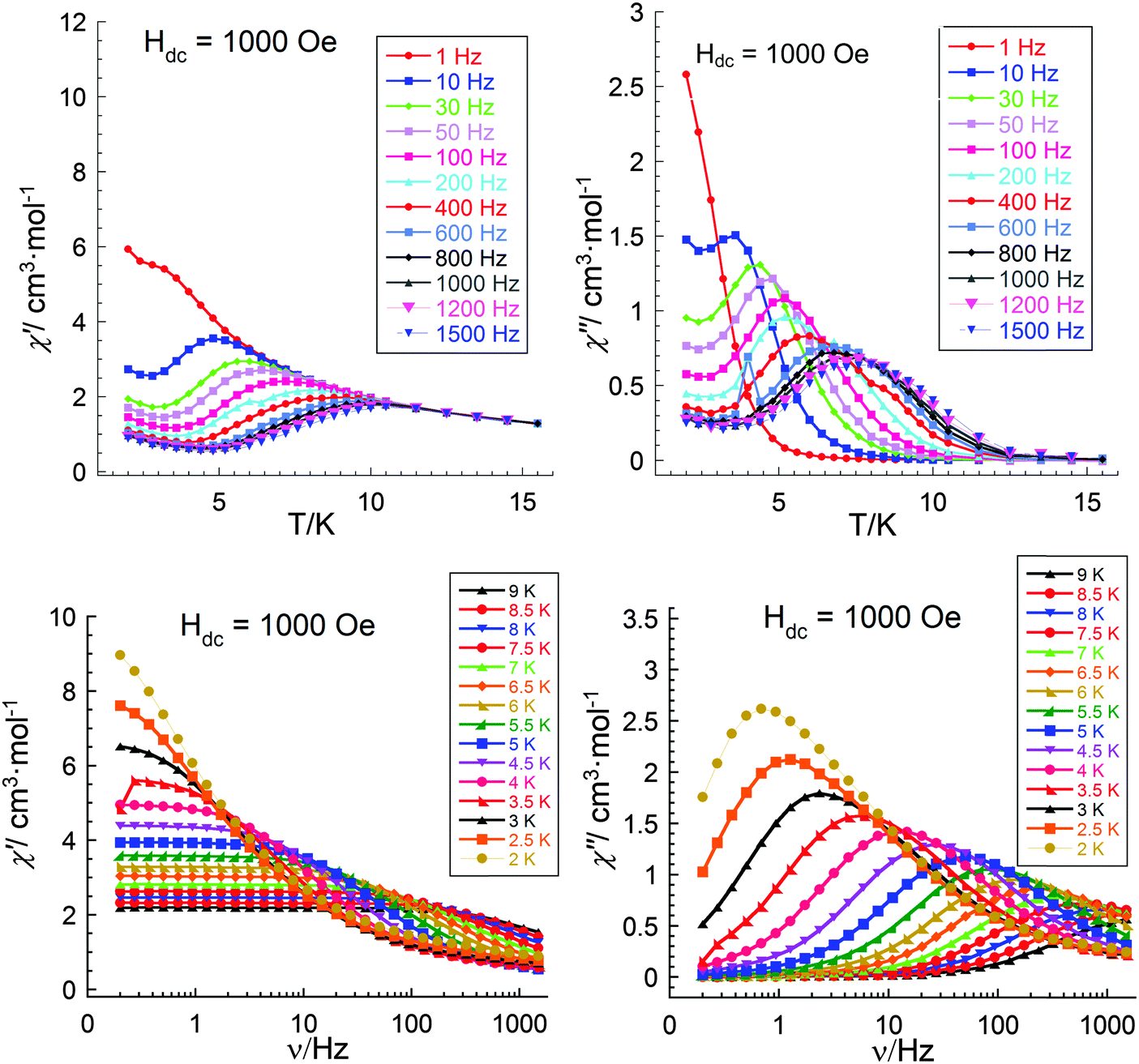
Fig. 5 Temperature dependence (upper) and frequency dependent (lower) of the in phase (left) and out-of-phase (right) components of the ac magnetic susceptibility at different frequencies for 1 (Fe₂Dy₂) at 1000 Oe.

Fig. 6 Arrhenius plot for 1 (Fe₂Dy₂) in 1000 Oe dc field.

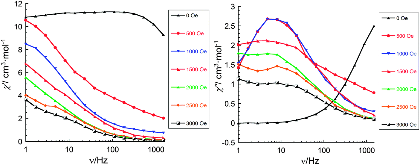
From the quick screening of the frequency dependence of the in-phase and out-of-phase components of the ac magnetic susceptibility (Fig. 4) it can be observed that at high fields (2000–3000 Oe) additional peaks develop with maxima which may lie at lower frequencies (0.1–1 Hz). These observations motivated us to revise our search for the optimal dc field. Therefore, a measurement was made using smaller increments between dc field values (Fig. 7 and 8). Remarkably, with increasing dc fields from 25 to 10 000 Oe we have observed three different relaxation processes: one at high frequencies (100–1500 Hz) and small fields (25–200 Oe), a second one at intermediate frequencies (1–100 Hz) and intermediate fields (200–800 Oe), and the third one at very small frequencies (0.1–1 Hz) and higher fields (1000–10 000 Oe). What is fascinating, is that with increasing dc field there is a gradual transition between these three processes and, simultaneously, gradual quenching of all of them. This result undoubtedly indicates that in compound 1 there are at least three relaxation processes with different relaxation times, which can be identified by non-zero dc field ac susceptibility measurements. At fields above 10 000 Oe the relaxation rate (due to the direct processes) is so fast that χ′′ can no longer be observed at frequencies below 1500 Hz (Fig. 8).

Fig. 7 Frequency dependence of the in- and out-of-phase components of the ac magnetic susceptibility for 1 (Fe₂Dy₂) at 2 K under different dc fields (0–2100 Oe).

Fig. 8 Frequency dependence of the in-phase and out-of-phase components of the ac magnetic susceptibility for 1 (Fe₂Dy₂) at 2 K under different dc fields (2600–10 000 Oe).

{YFe^III₂Y} (2). Here no frequency-dependent behaviour was observed in zero or 1000 Oe applied dc field. Hence, the Fe₂ fragment does not give rise to SMM behaviour, which is as expected since the antiferromagnetic Fe⋯Fe interaction leads to an S = 0 ground state.

{DyAl₂Dy} (3). In contrast to compound {DyFe^III₂Dy} (1), the temperature dependent χ′′ has a strong out-of-phase signal below 11 K at zero dc field with a maximum at 8 K for the highest frequency (ν) of 1500 Hz. The peaks in the frequency dependent χ′′ (Fig. 9) measurements become temperature independent below 3 K, indicating a possible quantum regime. The data for the corresponding measurements under an applied dc field 1000 Oe are shown in Fig. 10. At temperatures above 6 K the relaxation data is roughly linear and can be analysed using the Arrhenius law (Fig. 11) revealing very similar values for the thermal energy barrier to magnetisation relaxation of U_eff = 38.7 K and τ₀ = 1.06 × 10⁻⁶ s under zero field and U_eff = 41.5 K τ₀ = 9.95 × 10⁻⁷ s under an applied field of 1000 Oe. The barrier heights are thus significantly larger than the value of 16.2 K found from the analysis of the data obtained under an applied field of 1000 Oe for the Fe^III₂Dy₂ compound.

Fig. 9 Temperature dependence (upper) and frequency dependence (lower) of the in phase (left) and out-of-phase (right) components of the ac magnetic susceptibility for 3 (Al₂Dy₂) at zero applied dc field.

Fig. 10 Temperature dependence (upper) and frequency dependent (lower) of the in phase (left) and out-of-phase (right) components of the ac magnetic susceptibility for 3 (Al₂Dy₂) at 1000 Oe.

Fig. 11 Arrhenius plots for 3(Al₂Dy₂) under zero (left) and 1000 Oe (right) dc field.

The single crystal X-ray analysis shows that the molecules in all three compounds are centrosymmetric and it might be expected that there should not be any electronic differences between the individual Dy sites. This would imply that compounds 1 and 3 should show similar relaxation behaviour. Thus, since from the above studies we see different dynamic magnetic behaviour this must be related to the Dy–Fe exchange interactions in 1 which markedly decrease the U_eff barrier from that found for 3 and which in zero dc field becomes unquantifiable because the out-of-phase susceptibility signals lie at frequencies above the 1500 Hz we can apply with our SQUID. Thus, only on application of a dc field was it possible in compound 1 to slow down the relaxation processes and to extract the magnetic parameters. As mentioned above, to test how the dc field can affect the dynamic magnetic behaviour in compound 3, experiments with similar conditions to those for 1 were performed to investigate the temperature, χ′′(T), and frequency, χ′′(ν), behaviour under an applied field of 1000 Oe (Fig. 10). The obtained results are essentially the same as those obtained in zero dc fields (Fig. 9) and from the shapes of the χ′′(T), χ′′(ν) curves and Arrhenius plots (Fig. 11) one can conclude the presence in this compound of at least three relaxation processes. To prove this, a χ′′(ν) measurement in dc fields of 0–4000 Oe was performed (Fig. 12). As was found for {DyFe^III₂Dy} (1), on increasing the dc field, three clear transitions and their gradual quenching were observed. These observations suggest that the SMM behaviour for the {DyFe^III₂Dy} (1) and {DyAl₂Dy} (3) compounds arises from the presence of dysprosium ions in the molecules and that the different dynamic magnetic behaviour in dc field for 1 is attenuated by the presence of Fe^III–Dy^III exchange interactions in 1.

Fig. 12 Directions of the easy axes of the Dy ions (pink lines) in Al₂Dy₂ (3) as calculated using Magellan.¹⁶

Furthermore, an examination of the likely direction of the easy axes of the Dy^III ions in 3 using the Magellan software,¹⁶ reveals (Fig. 13) that these lie parallel to each other, as required by the centrosymmetric structure, and subtend angles of 53° to the Dy–Dy vector and 42° to the Al–Al vector. It can further be noted that the axis for Dy(1) is oriented almost along the Dy(1)–O(2) bond, such that it subtends angles of 29° and 78° with the Dy(1)–Al(1) and Dy(1)–Al(1′) vectors, respectively. We can therefore expect that in the Fe₂Dy₂ compound 1, the Fe site Fe(1) will be influenced mainly by the hyperfine field from Dy(1), whereas that at Fe(1′) will be mainly influenced by the field from Dy(1′).

Fig. 13 Frequency dependence of the in-phase and out-of-phase components of the ac magnetic susceptibility for 3 (Al₂Dy₂) at 2 K under different dc fields (0–4000 Oe).

Use of Mössbauer spectroscopy to provide a wider timescale for following the relaxation processes

Although in compound 1 the multiple relaxation processes could not be detected at zero-field for the ac magnetic measurements, and noting that the characteristic measuring time for such measurements is usually between ∼10 and 6.6 × 10⁻⁴ s, it was, however, possible to probe the situation on a different timescale using zero-field ⁵⁷Fe Mössbauer spectroscopy (Fig. 14(a–e)). ⁵⁷Fe Mössbauer spectroscopy provides a ∼10⁻⁷ s time window and it has been shown that this spectroscopy is useful not only for defining the total spin of iron entities in electronically very complicated Fe_xDy_y molecules,¹⁷ but also can give the spin structure of those entities and possible spin orientation of the Dy components of the molecules. Here we can extract the same information and show how this can provide very detailed microscopic information which cannot be extracted from other standard magnetic techniques for such challenging systems.

Fig. 14 (a–e) ⁵⁷Fe Mössbauer spectra of 1 (Fe₂Dy₂), at 3 K in zero- and applied external magnetic fields (0.1, 0.4, 1 and 2.5 T). (f–i) Frequency dependence of the out-of-phase ac susceptibility component for 1 (Fe₂Dy₂) at 2 K under different dc fields (0–10 000 Oe corresponding to 0–1 T). The correspondence between the results from the Mössbauer measurements and the ac susceptibility data can be seen by comparing the spectrum in (a) with the trace in (f); in (b) with the 1000 Oe trace in (h); in (c) with the 4000 Oe trace in (g) and in (d) with the 10 000 Oe trace in (i).

The form and characteristics of the Mössbauer spectra of the dinuclear Fe^III₂ unit prove an ideal probe of the low-temperature relaxation dynamics in the neighbouring Dy^III cations. For an ideal antiferromagnetic dimer (such as might exist in the {YFe₂Y}) the spin expectation value on each site is 0. However, if such an ideally isolated dimer were present in a cluster, this would be revealed by the magnetically split low temperature Mössbauer spectra and the two iron sites would give rise to zero hyperfine fields. An inspection of the Mössbauer spectrum at 3 K, zero field (Fig. 14(a)), suggests that in this complex the ferric sites exhibit considerable internal hyperfine fields of ∼9–12 T. While the obtained spectra look similar to the familiar six-line pattern of ⁵⁷Fe in a magnetically ordered state with intermediate relaxation time (relaxation spectra), the processes leading to the observed pattern are considerably more complex.

All attempts to simulate these spectra with a relaxation model failed. The fact that the pattern does not arise from relaxation effects could be confirmed by applying an external magnetic field. This should sharpen the magnetic lines, but here we see the completely opposite effect. The sextets start to vanish (see Fig. 14(b–d)) and at fields above 1 T (Fig. 14(e)) the Mössbauer spectra exhibit patterns typical of a diamagnetic complex.^8,9,13 These spectra cannot be modelled as a combination of a doublet and a sextet and the six lines cannot be reconciled with any single hyperfine pattern, again suggesting that multiple processes are in operation,

Normally, when an external magnetic field is applied to a simple antiferromagnetic iron compound, an individual sextet is typically broadened at small applied field. At larger applied field this is split into two sextets, one corresponds to the vector sum of the hyperfine field and the applied field (corresponding to the “normal” case at low applied fields) and the other to the vector difference.^18a Here, however, we see three overlapping magnetic patterns in the zero-field Mössbauer spectra. These can be explained by the presence of multiple relaxation processes within the Dy ions leading to the presence of three internal dipolar fields with different strengths and/or directions interacting with the ⁵⁷Fe nuclei.

An alternative scenario would be that what is observed is due to the resolution of the nuclear hyperfine structures corresponding to the various crystal field states of the ⁶S ion, Fe^III. However, the values for the observed internal field (9–12 T) are too small to arise from a mixture of the three possible states: M_S = ±1/2, ±3/2 and ±5/2, since the expected hyperfine fields for each component are ∼11, ∼33 and ∼55 T, respectively.¹⁸ Therefore we conclude that the magnetic patterns are molecule-based and result from slow intracluster relaxations in conjunction with internal molecular dipolar fields. These internal fields result from the non-reversal of the magnetisation mediated via ground and/or excited states M_J of the Dy^III ions at low temperature being sensed by the ferric cations.

An important further observation from the Mössbauer spectra is that there is no noticeable change in the pattern in the spectra measured between 0–1000 Oe (0–0.1 T) applied fields (Fig. 14(a and b)). Given the ∼10⁻⁷ s time window of Mössbauer spectroscopy this suggests that on this time scale no relaxation processes are affected by application of a field, whereas there is a clear change within the window of the ac-susceptibility measurements as shown in Fig. 14(f and h). On the other hand, when fields stronger than 1000 Oe are applied in the ac-susceptibility measurement, we can observe that the ac signals become broader (Fig. 14(g and i)) and also that the magnetic spectra in the Mössbauer start to disappear (Fig. 14(c and d)) with the finale occurring at 2.5 T. Here the antiferromagnetically coupled Fe₂ unit is able to dominate the magnetic structure of the cluster and is no longer influenced by the internal field from the Dy^III ions as a result of the very fast relaxation rate (faster than 10⁷ s⁻¹) of the magnetic states. At the intermediate field of 1 T (Fig. 14(d)) a clear minor magnetic onset is still seen in the Mössbauer spectra indicating the presence of a small component of slowly relaxing magnetic states within the Dy^III ions. This last observation is also supported by the ac data at 1 T which show a broad shoulder at low frequencies (Fig. 14(i)).

The observed effects from the magnetic and spectroscopic studies are expected, since on increasing the dc field we enhance the spin-phonon direct relaxation mechanisms of the Dy^III ions. Here the one-phonon relaxation between the two components of the doublets has rates which are proportional to the 3rd power of their Zeeman splitting, i.e., to the third power of the applied dc field (Oe). Usually, fields weaker than 1 T are enough to accelerate this relaxation.¹⁹

The presence in the Mössbauer spectra at 3 K of the two overlapping hyperfine patterns (doublet and sextet) with an approximate ratio of 50 : 50 is noteworthy since a similar effect has been observed in all the reported Fe^III₂Dy₂ compounds sharing the same core structure.^8,9,13 This is a clear indication of the presence of two different hyperfine interactions at the iron sites, but seems first sight at odds with the fact that the molecular structure suggests that the Fe centres are identical. This observation is, however, in line with a spin model where one Fe^III of the AF coupled dimer is aligned parallel and the other is antiparallel to the easy axes of the Dy ions.

As discussed above, from the Magellan analysis, the anisotropy directions on the Dy^III centres lie parallel to each other, but twisted with respect to the central metal dimer, at least for the analysis on the {DyAl₂Dy} compound 3. It can be noted that this result is also in line with the results from ab initio calculations performed on a structurally very similar {DyFe₂Dy} system.¹³ This thus implies that the spins on the central dimer are aligned antiparallel to each other along this anisotropy direction. We can also note that previous studies on related {LnFe₂Ln} systems, those where Ln = Gd have revealed that the antiferromagnetic Fe–Fe interaction is much stronger than the ferromagnetic Fe–Gd interaction and that the magnetic data can be fit using two J values.^13,20 In both studies the central Fe₂ unit was found to be strongly antiferromagnetically coupled and in one case the Fe–Gd interaction was found to be essentially zero²⁰ and in the other approximately 40 times smaller than the Fe–Fe interaction.¹³

It is of interest that in the former study,²⁰ a triangularly arranged {Fe₂Gd} system was also reported and in this case it proved necessary to analyse the magnetic data in terms of a frustrated system. From the magnetic data presented in Fig. 2 it can be seen that the low temperature χT vs. T data for Fe₂Dy₂ (1) and the “composite” data for {Fe₂Y₂ (2) plus Al₂Dy₂ (3)} essentially coincide, suggesting that also here the Fe–Dy interactions are very small compared with the central Fe–Fe interaction in the Fe₂Dy₂ compound 1. Thus we can safely rule out needing to apply a triangularly frustrated model to describe our observations and we suggest a different scenario.

From the experimental data, and in particular the insights from the Mössbauer spectroscopy, we can propose the following model to describe the magnetic dynamics and a possible magnetic structure for the core of 1. Firstly, we conjecture that the anisotropy axes for the ground and low lying Kramer doublets of both Dy^III ions are aligned in such a way that they are either parallel or antiparallel to the hyperfine fields at the central ⁵⁷Fe nuclei. Then, if the reversal of magnetisation of the two Dy^III ions occurs at a rate which is slower than approximately 10⁷ s⁻¹, the internal fluctuating dipolar fields will appear to be fixed within the timescale for the Mössbauer transitions. Since the central Fe^III₂ unit is an antiferromagnetically coupled dimer of two octahedral iron centres, it is most likely that the axial zero-field splitting parameter D > 0 and thus that the ground state is |±1/2〉. In magnetically diluted systems (e.g. 1–10% doping) the reversal of this spin at low temperatures should be slow and result in a resolved hyperfine structure corresponding to B_hf = 11 T.²¹ However, we can exclude this possibility, because compound 1 is not a magnetically diluted system and due to strong spin–spin interactions the relaxation in the |±1/2〉 state is very fast since it involves only a change of M_s of ±1 between the |+1/2〉 and the |−1/2〉 ground states. The only barrier for fast relaxation in this state is the presence of an internal molecular magnetic field arising from slow magnetisation reversal of the spins of the Dy^III ions. Since the main local magnetic axes on the Dy^III ions are co-parallel to each other as concluded from magnetic susceptibility measurements of the isostructural compound {DyAl₂Dy} (3) (Fig. 3), the Magellan analysis (Fig. 13), and from the previously reported ab initio results on a {DyFe₂Dy} compound analogous to 1,¹³ the relaxation in the |±1/2〉 state of the iron ion with the hyperfine internal field having the same direction as the magnetic field experienced from the non-reversal of magnetisation of two Dy^III neighbours will be slowed down. The field experienced at this iron site is a sensitive function of coordination geometry and main magnetic axes of the ground or/and excited Kramer doublets²² relative to the global field of the molecule. This would explain the observation of an average hyperfine field of ∼11 T determined from the magnetic onsets in 1, but the reason why a magnetic hyperfine interaction is only observed at one iron site is a puzzling feature requiring further study.

Conclusions

In conclusion, we have described the role of ⁵⁷Fe Mössbauer spectroscopy in understanding lanthanide anisotropy in Fe–Dy containing molecular clusters and how sensitive this method is for identifying very fine details of microscopic metal–metal communication and changes in the electronic structure of anisotropic weakly interacting lanthanide ions. For the first time we suggest an indirect approach for detecting the multilevel electronic nature of the Dy^III ions. From the Mössbauer spectra a superposition of several sextets is observed with the hyperfine fields originating from the interaction of the iron nuclei spin moments with the dipolar fields originating from magnetic substates of the Dy^III ions.

The effects observed in this study strongly suggest that under zero applied dc field the absence of the signal in the out of phase ac susceptibility experiments does not mean that the system is solely dominated by ground state magnetic tunnelling. Thus, other relaxation processes (e.g. direct, Orbach or Raman) are occurring, but are too fast to be detected by ac susceptibility measurements. However, they are slow enough to be sensed by the neighbouring iron nuclei and registered by Mössbauer spectroscopy, which probes magnetic relaxation on a much faster time scale. When dc fields (25 to ∼4000 Oe) are applied, then the relaxation of all these processes becomes slow enough for the peak maxima to fall within the frequency range of modern magnetometers, and, of course, still slow enough to be characterised by Mössbauer spectroscopy.

In short, we present a study which demonstrates the decisive role that the timescale of measurement techniques plays in helping to unravel the details of relaxation processes in magnetic materials.

Acknowledgements

We are grateful to the DFG TR-SFB88 “3MET” and the POF STN programme of the Helmholtz-Gemeinschaft for financial support.

References

1. R. L. Cohen, Application of Mössbauer Spectroscopy, V. II, Academic Press, New York, 1980.
2. (a) K. Liu, W. Shi and P. Cheng, Coord. Chem. Rev., 2015, 74, 289; (b) D. N. Woodruff, R. E. P. Winpenny and R. A. Layfield, Chem. Rev., 2013, 113, 5110; (c) P. Zhang, Y. N. Guo and J. Tang, Coord. Chem. Rev., 2013, 257, 1728; (d) F. Habib and M. Murugesu, Chem. Soc. Rev., 2013, 42, 3278; (e) J. D. Rinehart and J. R. Long, Chem. Sci., 2011, 2, 2078; (f) L. Sorace, C. Benelli and D. Gatteschi, Chem. Soc. Rev., 2011, 40, 3092; (g) C. R. Ganivet, B. Ballesteros, G. de La Torre, J. M. Clemente-Juan, E. Coronado and T. Torres, Chem. – Eur. J., 2013, 19, 1457; (h) J. W. Sharples and D. Collison, Coord. Chem. Rev., 2014, 60, 1; (i) R. Sessoli and A. K. Powell, Coord. Chem. Rev., 2009, 253, 2328; (j) J.-L. Liu, J.-Y. Wu, Y.-C. Chen, V. Mereacre, A. K. Powell, L. Ungur, L. F. Chibotaru, X.-M. Chen and M.-L. Tong, Angew. Chem., Int. Ed., 2014, 53, 12966.
3. (a) R. J. Blagg, C. A. Muryn, E. J. L. McInnes, F. Tuna and R. E. P. Winpenny, Angew. Chem., Int. Ed., 2011, 50, 6530; (b) R. J. Blagg, L. Ungur, F. Tuna, J. Speak, P. Comar, D. Collison, W. Wernsdorfer, E. J. L. McInnes, L. F. Chibotaru and R. E. P. Winpenny, Nat. Chem., 2013, 5, 673; (c) J. D. Rinehart, M. Fang, W. J. Evans and J. R. Long, J. Am. Chem. Soc., 2011, 133, 14236.
4. K. Mondal, A. Sundt, Y. Lan, G. E. Kostakis, O. Waldmann, L. Ungur, L. F. Chibotaru, C. E. Anson and A. K. Powell, Angew. Chem., Int. Ed., 2012, 51, 7550.
5. (a) G. Cucinotta, M. Perfetti, J. Luzon, M. Etienne, P.-E. Car, A. Caneschi, G. Calvez, K. Bernot and R. Sessoli, Angew. Chem., Int. Ed., 2012, 51, 1606; (b) S. K. Langley, D. P. Wielechowski, V. Vieru, N. F. Chilton, B. Moubaraki, B. F. Abrahams, L. F. Chibotaru and K. S. Murray, Angew. Chem., Int. Ed., 2013, 52, 12014.
6. E. Lucaccini, L. Sorace, M. Perfetti, J.- P. Costes and R. Sessoli, Chem. Commun., 2014, 50, 1648.
7. V. Mereacre, Angew. Chem., Int. Ed., 2012, 51, 9922.
8. A. Baniodeh, V. Mereacre, N. Magnani, Y. Lan, J. A. Wolny, V. Schünemann, C. E. Anson and A. K. Powell, Chem. Commun., 2013, 49, 9666.
9. V. Mereacre, A. Baniodeh, C. E. Anson and A. K. Powell, J. Am. Chem. Soc., 2011, 133, 15335.
10. C.-C. Wu, S. Datta, W. Wernsdorfer, G.-H. Lee, S. Hill and E.-C. Yang, Dalton Trans., 2010, 39, 10160.
11. (a) G. M. Sheldrick, Acta Crystallogr., 2015, A71, 3–8; (b) G. M. Sheldrick, Acta Crystallogr., 2015, C71, 3–8.
12. (a) M. L. Kahn, J.-P. Sutter, S. Golhen, P. Guionneau, L. Ouahab, O. Kahn and D. Chasseau, J. Am. Chem. Soc., 2000, 122, 3413; (b) M. L. Kahn, R. Ballou, P. Porcher, O. Kahn and J.-P. Sutter, Chem. – Eur. J., 2002, 8, 525.
13. A. Baniodeh, Y. Lan, G. Novitchi, V. Mereacre, A. Sukhanov, M. Ferbinteanu, V. Voronkova, C. E. Anson and A. K. Powell, Dalton Trans., 2013, 42, 8926.
14. N. F. Chilton, R. P. Anderson, L. D. Turner, A. Soncini and K. S. Murray, J. Comput. Chem., 2013, 34, 1164–1175.
15. (a) E. M. Pineda, N. F. Chilton, F. Tuna, R. E. P. Winpenny and E. J. L. McInnes, Inorg. Chem., 2015, 54, 5930; (b) J.-D. Leng, J.-L. Liu, W.-Q. Lin, S. Gomez-Coca, D. Aravena, E. Ruiz and M.-L. Tong, Chem. Commun., 2013, 49, 9341.
16. N. F. Chilton, D. Collison, E. J. L. McInnes, R. E. P. Winpenny and A. Soncini, Nat. Commun., 2013, 4, 2551.
17. (a) J. Bartolomé, G. Filoti, V. Kuncser, G. Schinteie, V. Mereacre, C. E. Anson, A. K. Powell, D. Prodius and C. Turta, Phys. Rev. B: Condens. Matter Mater. Phys., 2009, 80, 014430; (b) V. Mereacre, D. Prodius, Y. Lan, C. Turta, C. E. Anson and A. K. Powell, Chem. – Eur. J., 2011, 17, 123; (c) G. Abbas, Y. Lan, V. Mereacre, W. Wernsdorfer, R. Clérac, G. Buth, M. T. Sougrati, F. Grandjean, G. J. Long, C. E. Anson and A. K. Powell, Inorg. Chem., 2013, 52, 11767.
18. (a) E. Murad and J. Cashion, Mössbauer Spectroscopy of Environmental Materials and their Industrial Utilization, Springer, New York, 2004; (b) P. R. Locher and S. Geschwind, Phys. Rev., 1965, 139, A991.
19. L. Soeteman, A. J. van Duyneveldt, C. L. M. Pouw and W. Breur, Physica, 1973, 66, 63.
20. S. Mukherjee, M. R. Daniels, R. Bagai, K. A. Abboud, G. Christou and C. Lampropoulos, Polyhedron, 2010, 29, 54.
21. (a) G. K. Wertheim and J. P. Remeika, Phys. Lett., 1964, 10, 14; (b) H. H. Wickman and G. K. Wertheim, Phys. Rev., 1966, 148, 211; (c) J. W. G. Wignall, J. Chem. Phys., 1966, 44, 2462.
22. Y.-N. Guo, L. Ungur, G. E. Granroth, A. K. Powell, C. Wu, S. E. Nagler, J. Tang, L. F. Chibotaru and D. Cui, Sci. Rep., 2014, 4, 5471.

---

Footnote

† CCDC 1428524 and 1428525. For crystallographic data in CIF or other electronic format see DOI: 10.1039/c6cp02942f

---