Exploration of MOF nanoparticle sizes using various physical characterization methods – is what you measure what you get?

Abstract

While the size of nanoparticles (NPs) seems to be a concept established in the field of NPs and is commonly used to characterize them, its definition is not that trivial as different “sizes” have to be distinguished depending on the physical characterization technique performed to measure them. Metal–organic frameworks (MOFs) are known for their crystallinity, their large variety of compositions due to a huge number of inorganic building blocks that can be combined with almost endless organic linkers, their tunable pore structure, their ultrahigh porosity, and the different ways their backbones can be functionalised. The combination of these features with the nanoworld offers manifold perspectives for the synthesis of well-defined MOF nanoparticles (NPs), whose size attribute should be accurately determined as it strongly influences their physicochemical properties (at this length scale). In order to elucidate size determination, we synthesised zirconium fumarate metal–organic framework nanoparticles (Zr-fum MOF NPs) and characterized them using various common characterization methods. Herein, we compare the results of different solid-state methods, including powder X-ray diffraction (PXRD), atomic force microscopy (AFM), scanning electron microscopy (SEM) and transmission electron microscopy (TEM) to data obtained from dispersion-based methods, such as fluorescence correlation spectroscopy (FCS) and dynamic light scattering (DLS). In doing so, we illustrate the challenge of finding the appropriate method for obtaining a MOF NP size that is meaningful in the context of the desired application. Moreover, we demonstrate the importance of applying multiple complementary techniques as soon as the MOF NP size is considered. Throughout this paper, we highlight and define some reasonable recommendations of how the MOF NP size should be explored.

---

Introduction

Metal–organic frameworks (MOFs) are organic–inorganic hybrid crystalline compounds consisting of inorganic metallic clusters, also referred to as nodes, that are connected by organic linker molecules, i.e. spacers.^1–3 Owing to the many possible combinations of organic linkers and metal ions, a vast number of MOF structures, now up to more than 20 000, have been reported so far.³ Over the last few years, MOFs have attracted considerable scientific interest due to their wide structural and chemical tailorability,^4–6 their high surface area,^7–10 as well as the many possible different ways to functionalise their surface.^11–17 These characteristics have allowed for broad applications in various fields such as separation,¹⁸ storage,^19–22 catalysis,^23–28 sensing,^29–31 drug delivery,^32,33 diagnosis^32,33 and ionic conduction.³⁴ Furthermore, it has been shown that MOF crystal size can be controlled at the nanometre level to build MOF nanoparticles (MOF NPs).^35–45 Owing to the modular synthesis approach, together with spatial control of chemical moieties within the crystalline framework MOF chemistry offers, MOF NPs appear as a promising new class of functional NPs amongst the already existing NP material classes.

Control of MOF crystal size at the nanometre level results in MOF NPs whose properties are no longer determined by their inner surface only, but also by their outer surface properties, due to their high external surface-area-to-volume ratio.^46–50 When bulk materials are reduced to the nanometer size, their properties and their behaviour often become size- and shape-dependent. Examples of downsized MOF NPs and the resulting effects on their crystal structure and sorption behaviour are reported elsewhere.^51–53 Hence, the determination and the knowledge of both the size and shape of NPs are of paramount importance.⁵⁴ However, the obvious but important question – What is the “size” of a NP? – is not straightforward to answer as the “size” of a NP differs depending on what characterization technique is used and in which state the NP size is measured.⁵⁵ Various techniques relying on different physical principles and data processing methods are available to determine particle size and each one has its own advantages and drawbacks. In particular, once dissolved in solution, NPs interact with the solvent, e.g. by hydration, ion-adsorption,⁵⁶ or agglomeration,⁵⁷ and thus their effective size may significantly change.⁵⁸

In this article, the most widespread physical methods in the field of nanomaterial characterization, i.e. solid state methods, including X-ray diffraction (XRD), atomic-force microscopy (AFM), scanning electron microscopy (SEM) and transmission electron microscopy (TEM), as well as dispersion-based methods, such as dynamic light scattering (DLS) and fluorescence correlation spectroscopy (FCS), were applied to characterize and determine the size of zirconium-fumarate (Zr-fum) MOF NPs.^59,60Fig. 1 summarises the characterization techniques that contribute to determine the size of Zr-fum MOF NPs. The Zr-fum MOF NPs were synthesised based on a synthesis route reported by Behrens and co-workers (structural details of the Zr-fum MOF structure can be found in the ESI†).⁶¹ In that report, the authors showed that particle size could be controlled using formic acid as a modulator. The spherical morphology of the Zr-fum MOF NPs and the associated facile definition of the particle size (i.e. diameter) make the compound a prime example to showcase the various size determination methods.

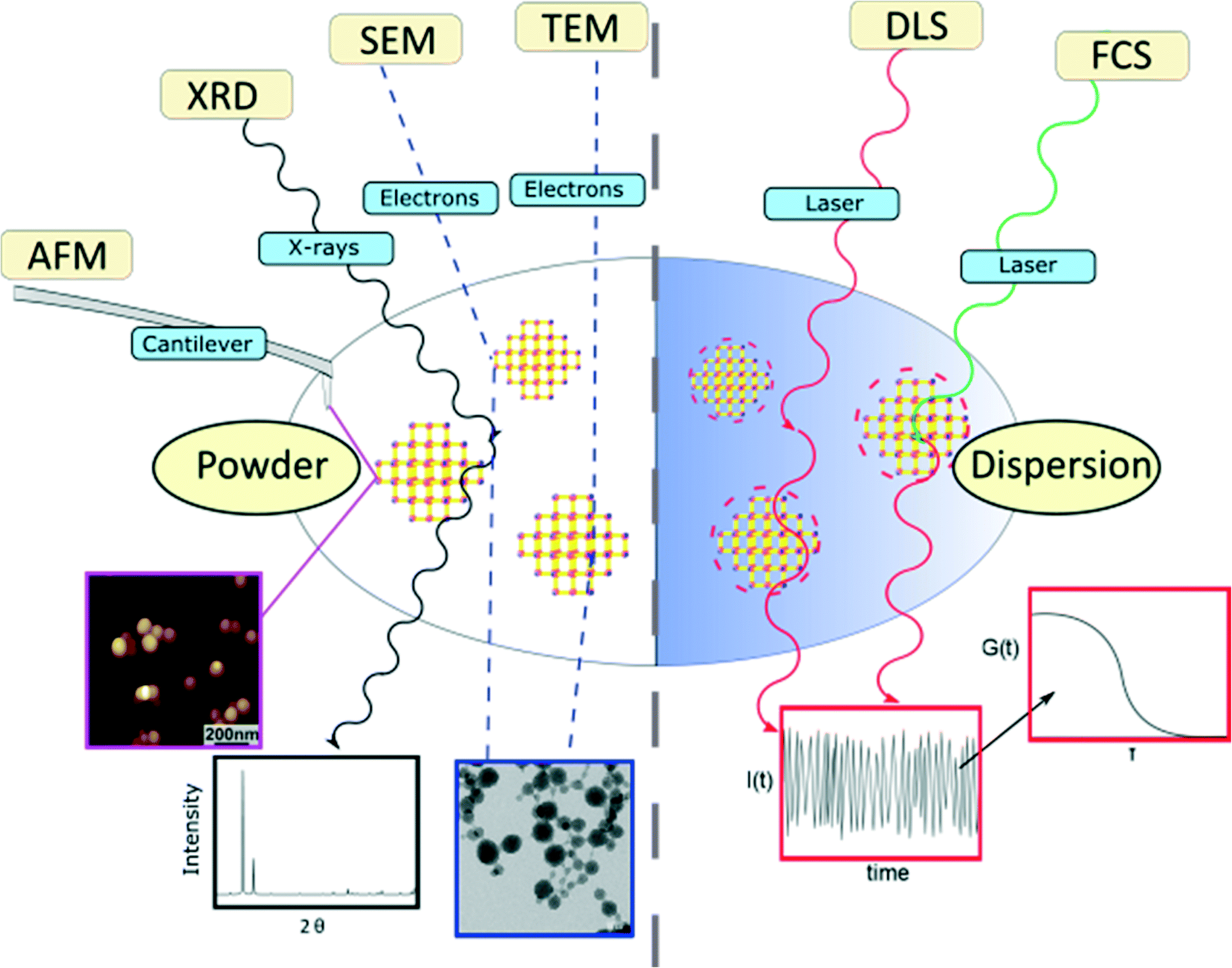Fig. 1 | Overview of the methods used to determine the size of Zr-fum MOF nanoparticles (atomic-force microscopy (AFM), X-Ray diffraction (XRD), transmission electron microscopy (TEM), scanning electron microscopy (SEM), dynamic light scattering (DLS) and fluorescence correlation spectroscopy (FCS)).

In this work, we briefly discuss the physical principle of each size characterization method and show each method's practical advantages and disadvantages in NP size assessment. Then, we compare the various “sizes” obtained for the Zr-fum MOF NPs using the different techniques and finally, we discuss the meaning and appropriateness for MOF NP characterization in general.

Results

The Zr-fum MOF NPs were synthesised using the same approach used by Behrens and co-workers.⁶¹ The synthesis is carried out solvothermally in water using ZrCl₄ substrates and fumaric acid (see the ESI† for more details). In the subsequent section, we first display the results of solid-state based methods such as SEM, TEM, AFM and XRD. Even for those methods, the experimental conditions of measurements may be very different. While TEM requires operation in vacuum, for example, AFM could be carried out in a fluid cell on NPs adsorbed on a surface. In addition to determination of particle size, all the techniques offer some different advantages of identifying Zr-fum MOF NPs, such as confirming their crystallinity and determining their 2- or 3-dimensional morphology. Thereafter, the outcomes of dispersion-based methods such as DLS and FCS, which need to be carried out in the liquid phase, are showcased. Those techniques are suitable for studying NP properties such as their aggregation behaviour and their hydrodynamic diameters, which are specific to dispersions.

Scanning electron microscopy (SEM)

Scanning electron microscopy is one of the most widely used techniques to characterise nanomaterials. This method relies on the use of an electron beam, whose energy is around 5 keV, that scans the surface of a solid sample. The electrons of the focused incident beam impinge on the sample surface and generate secondary electrons, which are collected using a detector and used to create the sample image. SEM analyses were performed on a sample that was prepared by drying an ethanol-based dispersion of Zr-fum MOF NPs followed by carbon-sputtering. They reveal the spherical morphology of the NPs, as shown in Fig. 2a. The size distribution of the Zr-fum MOF NPs was determined by measuring the diameter of approximately 1000 NPs (Fig. S4†). The resulting values were plotted in a histogram and fitted with a Gaussian function (Fig. 2b) centred on an average NP diameter of d^SEM_Zr-fumNPs = 62.0 ± 18.9 nm. It is worth noting that SEM requires conductive substrates in order to avoid charging effects, and thus a non-conductive Zr-fum MOF NP sample should be sputtered with a conductive film before being analysed.

Fig. 2 | Characterisation of Zr-fum MOF NPs with different methods: (a) SEM micrograph; (b) particle size distribution of Zr-fum MOF NPs from SEM images (Fig. S4†); (c) TEM micrograph; (d) electron diffraction pattern of Zr-fum MOF NPs; (e) particle size distribution of Zr-fum MOF NPs from TEM images (Fig. S9–S13†); (f) AFM micrograph; (g) particle size distribution of Zr-fum MOF NPs from AFM images; (h) experimental PXRD pattern of the Zr-fum-3 MOF NPs (black symbols), Pawley fit (red), Bragg positions (green symbols) and the difference between the Pawley fit and the experimental data (dark green). The observed reflection intensities are in very good agreement with the simulated PXRD pattern (blue) based on the Pn-3 symmetry of the Zr-fum MOF structure model.⁵³

Transmission electron microscopy (TEM)

In the transmission electron microscopy experiment, a high-energy electron beam (E ∼200 keV) is focused on a thin sample (typically less than 200 nm) made of a carbon grid on which a droplet of a NP suspension has been evaporated. The electrons passing through the sample, in other words being transmitted, are scattered at different angles and are then focused with a lens system on a detector to achieve micrographs with a high lateral spatial resolution. TEM offers the important advantages of high magnification, ranging from 50 to 10⁶ and the ability to provide both image and diffraction pattern information. The latter one is especially crucial for MOF NPs, as it proves the crystallinity of the structure. A typical TEM micrograph of Zr-fum MOF NPs is depicted in Fig. 2c and proves the spherical shape of the NPs. Moreover, this picture also shows that the NPs are interconnected via necks. The histogram shown in Fig. 2e reports the distribution of NP diameter, which was measured on approximately 1000 individual specimens (Fig. S9–S13†). The adjustment of this distribution with a normal law gives rise to an average NP diameter with a standard deviation of d^TEM_Zr-fumNPs = 29 ± 12.9 nm.

Fig. 2d shows the electron diffraction pattern of the Zr-fum MOF NP sample. The radial distance of the apparent spots indicates the lattice distance in reciprocal space. A comparison among the tabulated values for the Zr-fum MOF crystal structure shows very good agreement (see Table S4†). Although no crystal fringes are displayed in Fig. 2c, the Debye–Scherrer rings shown in Fig. 2d prove the crystallinity of the sample. Upon prolonged exposure to the high-energy electron beam (200 keV), the Debye–Scherrer rings gradually disappear over an exposure time of around 30 s (Fig. S6–S8†). This indicates that the sample is damaged resulting in loss of the Zr-fum MOF NP crystallinity (Fig. 2c). However, the electron diffraction pattern shown in Fig. 2d was generated from a larger sample area, causing the rate of the impinging electrons to be lower and the sample to be destroyed much slower.

Atomic force microscopy (AFM)

In atomic force microscopy, the sample is analysed by rasterising its surface with a sharp tip attached to a cantilever. In our case, the measurements were performed in a closed loop tapping mode in air, in which the cantilever is excited to vibrate close to its resonance frequency using a piezoelectric device. The interactions between the cantilever-tip and the sample surface, i.e. repulsive Coulomb forces and attractive van der Waals forces, change the amplitude of the cantilever oscillation. A feedback loop constantly adjusts the height of the cantilever to maintain a defined oscillation amplitude, whose variations are used to generate a topographic image of the sample. Fig. 2f displays the AFM micrograph of a Zr-fum MOF NP sample prepared by drying an ethanolic NP-dispersion on a SiO₂ slide. Apart from individual NPs, we also observe agglomerated NPs, which can come from the sample preparation. In order to obtain the size of individual particles, the measurements were realised in the outermost periphery of the dried droplet were the density of the particles is minimised. From the AFM images, particle sizes have been determined statistically using the particle and pore analysis tool integrated in the Scanning Probe Image Processing (SPIP) (see the ESI†). The NP height distribution is plotted in Fig. 2g. The Gaussian curve fit is centred on an average NP diameter of d^AFM_Zr-fumNPs = 68 nm with a standard deviation equal to 15 nm.

X-Ray diffraction (XRD)

In X-ray diffraction experiments, the elastic diffraction of X-rays on the atoms of a solid sample is used to identify its atomic and molecular structure. The Scherrer equation relates the broadening of a peak in a powder diffraction pattern to NP size and is therefore applied to calculate NP diameter (see the ESI†). As MOFs are crystalline materials, the determination of crystallite size and its comparison to particle size is of interest, since it can be used to estimate if single crystals or polycrystals are dominant in a sample.

The powder X-ray diffraction (PXRD) patterns of the Zr-fum MOF NP samples feature well-defined reflections across the entire measurement range, indicating the formation of well-ordered frameworks (Fig. 2h and Fig. S14†). Moreover, the experimental reflection intensities match the simulated pattern based on the reported Zr-fum structure⁶¹ (blue line in Fig. 2h) very well, thus confirming the formation of a cubic Zr-fum MOF.

Analysis of PXRD data is commonly performed via Pawley fitting.⁶² This method compares a theoretical diffraction pattern derived from a structure model to the corresponding experimental data, and varies unit cell parameters and peak profiles until convergence criteria are reached. Unlike the Rietveld method, Pawley fitting treats peak areas as variables, thus rendering this method also applicable to patterns recorded in reflection geometry, at the cost of not being able to refine atomic positions. We used the Pawley method to extract the lattice parameter a from the reflection positions and the average crystal domain size d from the peak broadening (see the ESI† for details).

Pawley fitting using the above mentioned structure model led to a lattice parameter a ranging from 17.88 ± 0.03 Å to 17.91 ± 0.03 Å for the Zr-fum MOF NP samples (ESI,† Fig. S14), which are very similar to the lattice parameter of 17.91 Å that has been reported for the bulk material.⁶¹ We then extracted the average crystal domain size d from the peak broadening taking into account the instrument broadening and the line shapes (see Section 2 “X-ray Diffraction” in the ESI† for details). This domain size ranges from d^XRD_Zr-fumNPs = 42 ± 5 nm to 60 ± 5 nm.

In contrast to the other methods discussed above, XRD analysis provides the size of crystalline domains rather than the geometrical shape. In the case of defect-free single-crystalline NPs, these two quantities would be identical. In reality, a fraction of NPs will feature grain boundaries or other defects that disrupt the periodicity of the crystal. The average domain size of the NP powder sample will thus be smaller than the average particle size as determined by TEM, for example.

With the presentation of the results stemming from the solid-state based methods being finished, the outcomes of the dispersion-based methods are broached in the following paragraphs. It is worth noting that the results of these methods may strongly depend on the solvent in which the NPs are dispersed.

Dynamic light scattering (DLS)

Dynamic light scattering is probably the most frequently used technique for determining the hydrodynamic diameter of particles, which is defined as the “size” of a hypothetical homogeneous hard sphere that diffuses in the same fashion as that of the particle being measured. The working principle of DLS relies on measuring the intensity fluctuations caused by interference of laser light that is scattered by diffusing particles. Temporal evolution of the fluctuations depends on the particle movement caused by Brownian motion. It is therefore correlated to the diffusion coefficient of NPs, which depends on their size. When tracing this intensity over time, it is possible to plot a second order autocorrelation function. From this autocorrelation function, the diffusion coefficient of a particle can be retrieved using a fitting model. However, caution should be taken as the resultant computed hydrodynamic diameter is dependent on the chosen fit model, which typically is hidden as a black-box in a machine.⁶³ In our study, the average hydrodynamic diameter of Zr-fum MOF NPs was first determined in water (see Fig. 3b (black)) to have a good comparability with similar FCS measurements (see next section). Subsequently, the particles were examined in ethanol (see Fig. 3b (red)) to show the NPs behaviour in such a typical solvent (see the ESI†). Diluted dispersions of the NPs were analysed, and the resulting autocorrelation function was fitted using the “method of cumulants” (for more details, see the ESI†). In water, this resulted in NPs featuring a hydrodynamic diameter of d^DLS_Zr-fumNPs = 42 nm with a standard deviation of σ = 46 nm. In ethanol, their hydrodynamic diameter was equal to d^DLS_Zr-fumNPs = 130 nm and with a standard deviation of σ = 48 nm.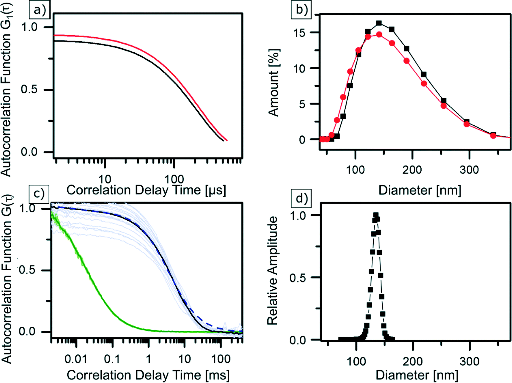

Fig. 3 | DLS correlation data (a) and size distribution (b) of Zr-fum MOF NPs in ethanol (red) and water (black) as well as averaged and normalised FCS autocorrelation curves (c) of Alexa Fluor 488 (green) and labelled Zr-fum MOF NPs in water (black), greyed out curves are underlying single measurements. GDM fit (dashed blue curve) results in a size distribution (d) at a peak diameter of 135 nm, considering finite size correction.⁵⁶

Fluorescence correlation spectroscopy (FCS)

Fluorescence correlation spectroscopy is a fluorescence-based method which is used to determine the hydrodynamic diameter of labelled NPs.^64,65 In this method, a laser is confocally focused into a liquid sample containing fluorescently labelled NPs. Fluorescence intensity fluctuations, resulting from NPs traversing an excitation volume, are recorded using an avalanche photodiode and used to calculate the time autocorrelation function. FCS data analysis yields the diffusion coefficient as well as the concentration of fluorescent particles (see the ESI†). Using the Stokes Einstein relation, the NP hydrodynamic diameter is calculated from the measured diffusion coefficient. Three samples of Zr-fum MOF NPs were labelled with the dye Alexa Fluor 488 (absorption at 488 nm and emission at 519 nm) and were examined with FCS. The normalised autocorrelation functions, shown in Fig. 3c, correspond to one of the labelled Zr-fum MOF NP samples (black). For comparison, the autocorrelation of free Alexa Fluor 488 is shown in green. Normalisation helps to clearly visualise that the autocorrelation function of the dye-labelled NPs is shifted towards higher correlation times with respect to the free Alexa Fluor 488 molecules. This indicates slower diffusion of the particles due to the larger hydrodynamic diameter of the NPs. Using a single component fit model (see the ESI†) results in an apparent diffusion time of 3.68 ms, which corresponds to a hydrodynamic diameter of d^FCS_Zr-fumNPs = 135 nm after using the finite particle size correction for hollow spheres presented by Wu et al.⁶⁶ The fit (not shown) is reasonable at lag times τ < 10 ms but deviations from the data show that the model of the monodisperse particles is not satisfactory and indicate that there is a broad distribution of the particle size. Thus, the Gaussian Distribution Model (GDM)^67,68 was used to fit the data. The GDM fit (dashed blue line in Fig. 3c) results (again, after finite size correction) in a peak diameter of d^GDMFCS_Zr-fumNPs = 135 nm and a FWHM of 17 nm (see Fig. 3d).

Discussion

As stated in the introduction, the concept of the “size” of a NP is intangible since each characterization technique provides its own NP size, which differs from one method to another. This concept becomes clearer when considering on the one hand the different physical principles governing the methods and on the other, the state of the analysed sample.

Herein, the employed characterization techniques were divided into two categories, depending on whether the samples are analysed in the dry state or in a dispersion (Fig. 1). Measuring NPs in the dry state, i.e. as a powder, has the crucial disadvantage that it is hard to distinguish between aggregated NPs resulting from the sample preparation itself or agglomerates that were already present before. The agglomeration of NPs is energetically favoured as it minimizes surface areas and can saturate bonds and coordination sites.⁶⁹ Therefore, one should exercise caution when determining the NP size distribution from powder based-techniques and assuming the existence of individual NPs. In particular, in the case of promising biomedical applications of MOF NPs as nanocarriers or diagnostic agents or even both, non-agglomerated and colloidally stable MOF NPs are required and thus, their characterization in the liquid state is mandatory to clarify their aggregation state.

SEM, TEM and AFM microscopy techniques provide an image of NPs from which the diameters as well as the shape of NPs are easily extracted. All the microscopy techniques revealed the spherical shape of Zr-fum MOF NPs (Fig. 2). To give a representative insight into the NPs' diameter, a statistical study must be performed on a sufficient number of NPs, independent of the used technique. In this work, the diameter of 1000 NPs for TEM and SEM and of 500 NPs for AFM has been measured on the recorded images (see the ESI† Fig. S4, S9–13). A difficulty encountered in the SEM images is the identification of individual particles (see Fig. S4†). Small particles are easily overlooked, which might shift the resulting NP diameter distribution to higher values. TEM allows the detection of smaller NPs due to its larger spatial enhancement compared to SEM. In the TEM pictures of Zr-fum MOF NPs (Fig S9–13†), it is clearly visible that the NPs are connected together via thin necks, which were not taken into account to evaluate the NP diameter. However, one may argue that neck-connected NPs actually originate from agglomeration. Moreover, NPs featuring diameters smaller than the diameter of the thin necks, which connect larger NPs, may be overlooked when two-dimensional TEM images are analysed.

In high quality TEM micrographs of MOF NPs, it is normally possible to detect crystal fringes showcasing the crystallinity of the respective MOF structures.⁴⁵ In the case of the Zr-fum MOF NPs, this was not feasible due to beam damage. However, the crystallinity of MOF NPs was unambiguously proven using HRTEM by examining electron diffraction patterns (Fig. S8–S10 and Table S4†). Beam damage of a sample is a known problem in TEM mostly with high-energy electron beams (E > 100 keV). Further, it can be stated that the Zr-fum MOF NPs are highly beam sensitive, since the MOF NPs lose their crystallinity over a time frame of 30s (Fig. S8–S10†). Loss of the MOF NP crystallinity goes together with shrinking, which also explains the shift of the particle size distribution to lower values when comparing the TEM and SEM results (Table 1). Therefore, for the Zr-fum MOF NPs, TEM analysis is not suitable for measuring the size distribution, but suitable to confirm the crystallinity of the sample (Table S4†).

Table 1 | Summary of the average diameters of spherical Zr-fum MOF NPs obtained using three different microscopy tools and three different spectroscopic methods. The standard deviation is also reported

	Method	Type of sample	Measured quantity	Average diameter (nm)	Standard deviation (nm)
a This method does not give a particle size distribution but results in a mean size assuming a single species.
Microscopy	SEM	Dried on a carbon support	Diameter	62	18.9
	TEM	Dried on a carbon grid	Diameter	29	12.9
	AFM	Dried on a silica slide	Height	68	15.0
Spectroscopy	XRD	Powder	Domain diameter	42–60	—^a
	DLS	Dispersion (H2O)	Hydrodynamic diameter	142	46
	FCS	Dispersion (H2O), labelled	Hydrodynamic diameter	135	17 (FWHM)

---

The NP diameter distribution obtained using AFM is in good agreement with the one obtained from SEM measurements (Table 1). Contrary to SEM and TEM techniques, the contrast between the Zr-fum MOF NPs and the object slide (SiO₂) was sufficient to analyse the size of individual particles via an imaging software. Another advantage of AFM over SEM and TEM is the gentle nature of this method, which relies on the interaction of a cantilever tip with the particle surface instead of using a high electron energy beam.

Comparing the results of the X-ray diffraction experiments to the AFM and SEM results, similar diameters are measured. In contrast to SEM, TEM and AFM, which all result in NP diameter distributions, X-ray diffraction gives the average size of the sample crystalline domains, which are not necessarily equal to the NP size. Since the resulting value is an average only, no particle size distribution is obtained. The various possible NP species, which may lead to this average value, are not taken into account. In theory, the average crystalline domain size could result from two sample species, each featuring a uniform size. Alternatively, the average crystalline domain size may result from a broad particle size distribution. If all sample particles are not expected to be single crystals due to the presence of an amorphous material, one would expect the crystalline domain size to be shifted towards smaller values in comparison to NP diameter.

Additionally, defects in the crystal structure result in peak broadening. Since the crystalline domain size is calculated from the width of these peaks, this causes the former to shift towards smaller values. The good agreement among AFM, SEM and X-ray diffraction results suggests the presence of highly crystalline Zr-fum MOF NPs, whose crystal domain size is similar to the NP diameter. Finally, the sharp reflections and very small background observed in the X-ray diffraction experiments also prove the high crystallinity of the sample, complementing the results of TEM measurements.

The outcome of DLS and FCS is a distribution of diffusion coefficients D, which is then transformed into a distribution of hydrodynamic diameters, i.e. diameters of those spheres that yield the same D-values. Therefore, the hydrodynamic diameter does not describe the morphology of a particle but the chosen fitting model assuming a solid sphere or another ideal geometric shape, which has the same diffusion properties as the measured particle. As the Zr-fum MOF NPs feature a rather good spherical morphology, and as no additional organic surface capping is used, the values obtained from the dispersion-based methods should to some extent be comparable to those obtained from the powder methods. However, the hydrodynamic diameter of the Zr-fum MOF NPs determined using DLS and FCS is significantly larger than the NP diameters determined with the powder-based methods (Table 1).

In the case of DLS measurements, substantial absorption of laser light (λ = 633 nm) by a sample itself, which causes a systematic measurement error, can be ruled out by our white Zr-fum MOF NPs. Hence, the differences in the measured NP size values can be explained by the presence of small aggregates. FCS measurements reveal hydrodynamic diameters close to those obtained using DLS but with a narrower distribution. This can be explained by different fitting models. However, both methods disclose the presence of agglomerates of the Zr-fum MOF NPs in solution as the NP diameter determined by the solid techniques is significantly smaller. Functionalisation of MOF NPs with appropriate organic surface cappings, providing either electrostatic or steric repulsion, could help reduce the amount of aggregates.

Conclusion

One of the key issues in NP research is that the product of a chemical synthesis of NPs is a colloidal dispersion, which exhibits a polydisperse distribution of sizes and shapes, rather than a collection of identical NPs. This is the main reason why the reproducibility of NP synthesis results is so difficult to ensure, even if the same person carries out the synthesis under the same experimental conditions. For this reason, a careful and extensive NP characterization is required. Moreover, future NP database will collect physical dispersion data together with the chemical composition of NPs. Such kind of database is important as it allows researchers to compare different NP data sets and also to put their own results in place. For this reason, recommendations for MOF NP characterization using standard physical characterization tools have been introduced. Zr-fum MOF NPs appeared as ideal candidates to reach this fixed target owing to their perfect spherical shape. In our work, we applied six characterisation methods on Zr-fum MOF NPs and the obtained results were discussed and compared based on the underlying physical process of the characterisation device.

When choosing techniques to characterise a nanomaterial, it is important to bear in mind the later usage of the respective compound. Powder characterisations with SEM, TEM or AFM are essentially sufficient when considering solid based-applications of MOF NPs. However, in solution-based applications such as drug delivery, colloidally stable NP solutions are required, which must thus be characterised in solution with DLS and/or FCS, for instance. Since these methods do not give insight into the morphology of NPs, it is therefore advantageous to complement these techniques by an image-providing technique such as TEM, SEM or AFM.

In the case of MOF NPs, the determination of crystallinity and in particular the quantification of the crystalline domain size is an important parameter. However, the XRD patterns of MOF NPs need to be carefully analysed as high-crystallinity or even the existence of a MOF structure cannot always be stated due to the potential broadening of peaks in an XRD pattern. For example, the crystallinity of MIL-101(Cr) and MIL-100(Fe) NPs is unequivocally proven by TEM analysis only.⁴⁸ In comparison to the tested Zr-fum MOF NPs, the respective MOF NPs in those cases were more beam stable. The difficult characterisation of MOF NPs that are sensitive to the electronic beam of TEM could be overcome with the new versions of TEM instruments operating at lower voltage (e.g. 60 keV).

TEM analysis usually appears as the most suitable method to determine the size of isolated MOF NPs in the dry state due to its high spatial resolution. However, as shown in the case of the Zr-fum MOF NPs, beam damage can spoil the outcome, making TEM no longer appropriate. SEM represents a good alternative to TEM because it operates at a much lower voltage even if small NPs (<20 nm) of a sample can be hardly detected since they are hidden by bigger ones. TEM and SEM pictures were used to manually determine the Zr-fum MOF NP size distribution. Although this is time consuming, this approach is sufficient when having spherical NPs but cannot be applied to non-spherical NPs.

Many MOF NP applications need dispersions of colloidally stable MOF NPs. Even though most researchers target solution-based NP applications (e.g. drug delivery), they often do not furnish evidence on the colloidal properties of MOF NPs. This enigma comes from agglomeration issues often met with nanomaterials. The chemistry of every NP material class, including MOF NP, faces the challenge of synthesising colloidally stable NPs. The saturation of a MOF NP surface immediately after MOF NP nucleation, either by electrostatic repulsion or steric stabilisation, can avoid this agglomeration issue. A stable MOF NP suspension can be easily characterised by DLS analysis, whereby caution should be paid to the automatic evaluation of the size distribution of the instrument. An alternative solution to DLS is FCS, as demonstrated in this article. FCS is based on evaluation of a autocorrelation function to obtain the diffusion coefficient of fluorescence-labelled NPs. Although FCS has the disadvantage of requiring dye labelled NPs, meaning that they are chemically modified, in many applications, such as drug delivery or diagnosis, NPs need to be labelled for the application itself, e.g. to carry out cell uptake studies. In these cases, FCS is an excellent characterisation technique due to its high spatial and temporal resolutions and its ability to analyse extremely low NP concentrations (nM to pM concentrations) in a very small volume (∼0.1 fL). Consequently, a low amount of sample is needed to precisely determine the hydrodynamic diameter of labelled NPs. Moreover, FCS measurement simultaneously provides information about the concentration (inverse correlation height) of the investigated sample.

In summary, we presented comprehensive physical characterization of the size, shape and bulk properties of Zr-fum MOF NPs. Evidently, the structural properties of MOF NPs provide a large set of parameters allowing for a thorough assessment of MOF NP quality. Future applications that will exploit MOF NPs as hosts, delivery vehicles or catalytic agents rely on the full knowledge of their physical NP properties. The caveats and peculiarities in NP size characterisation discussed here might help for standardisation and better comparability of MOF NP properties.

Acknowledgements

The authors are grateful for financial support from the Deutsche Forschungsgemeinschaft (DFG) through SFB 1032 and DFG-project WU 622/4-1, the Excellence Cluster Nanosystems Initiative Munich (NIM), the Center for NanoScience Munich (CeNS), and the European Commission (project FutureNanoNeeds). Authors AP and JV gratefully acknowledge financial support from the DFG within the RTG 1782 “Functionalization of Semiconductors”. Furthermore, we thank Steffen Schmidt and Michael Beetz for TEM measurements, and Beatriz Pelaz, Neus Feliu, and Pablo del Pino for helpful technical discussions. Last but not least, SW thanks Dr. M. Lismont (University of Liège) for valuable discussions and comments.

Notes and references

1. S. Kitagawa, R. Kitaura and S.-I. Noro, Angew. Chem., Int. Ed., 2004, 43, 2334–2375.
2. G. Férey, Chem. Soc. Rev., 2008, 37, 191–214.
3. H. Furukuwa, K. E. Cordova, M. O'Keeffe and O. M. Yaghi, Science, 2013, 341, 974–987.
4. W. Lu, Z. Wei, Z.-Y. Gu, T.-F. Liu, J. Park, J. Park, J. Tian, M. Zhang, Q. Zhang, T. Gentle Iii, M. Bosch and H.-C. Zhou, Chem. Soc. Rev., 2014, 43, 5561–5593.
5. T. R. Cook, Y.-R. Zheng and P. J. Stang, Chem. Rev., 2013, 113, 734–777.
6. D. J. Tranchemontagne, J. L. Mendoza-Cortés, M. O'Keeffe and O. M. Yaghi, Chem. Soc. Rev., 2009, 38, 1257.
7. O. M. Yaghi, M. O'Keeffe, N. W. Ockwig, H. K. Chae, M. Eddaoudi and J. Kim, Nature, 2003, 423, 705–714.
8. I. Senkovska and S. Kaskel, Chem. Commun., 2014, 50, 7089.
9. R. Grünker, V. Bon, P. Müller, U. Stoeck, S. Krause, U. Mueller, I. Senkovska and S. Kaskel, Chem. Commun., 2014, 50, 3450.
10. O. K. Farha, I. Eryazici, N. C. Jeong, B. G. Hauser, C. E. Wilmer, A. A. Sarjeant, R. Q. Snurr, S. T. Nguyen, A. Ö. Yazaydın and J. T. Hupp, J. Am. Chem. Soc., 2012, 134, 15016–15021.
11. P. Deria, J. E. Mondloch, O. Karagiaridi, W. Bury, J. T. Hupp and O. K. Farha, Chem. Soc. Rev., 2014, 43, 5896–5912.
12. J. D. Evans, C. J. Sumby and C. J. Doonan, Chem. Soc. Rev., 2014, 43, 5933–5951.
13. S. M. Cohen, Chem. Rev., 2012, 112, 970–1000.
14. H. Furukawa, U. Müller and O. M. Yaghi, Angew. Chem., Int. Ed., 2015, 54, 3417–3430.
15. H. Hintz and S. Wuttke, Chem. Mater., 2014, 26, 6722–6728.
16. H. Hintz and S. Wuttke, Chem. Commun., 2014, 50, 11472–11475.
17. S. Wuttke, C. Dietl, F. M. Hinterholzinger, H. Hintz, H. Langhals and T. Bein, Chem. Commun., 2014, 50, 3599.
18. B. Van de Voorde, B. Bueken, J. Denayer and D. De Vos, Chem. Soc. Rev., 2014, 43, 5766–5788.
19. S. Van der Perre, B. Bozbiyik, J. Lannoeye, D. E. De Vos, G. V. Baron and J. F. M. Denayer, J. Phys. Chem. C, 2015, 119, 1832–1839.
20. S. Van der Perre, T. Van Assche, B. Bozbiyik, J. Lannoeye, D. E. De Vos, G. V. Baron and J. F. M. Denayer, Langmuir, 2014, 30, 8416–8424.
21. Y. He, W. Zhou, G. Qian and B. Chen, Chem. Soc. Rev., 2014, 43, 5657–5678.
22. J. Canivet, A. Fateeva, Y. Guo, B. Coasne and D. Farrusseng, Chem. Soc. Rev., 2014, 43, 5594–5617.
23. J. Lee, O. K. Farha, J. Roberts, K. A. Scheidt, S. T. Nguyen and J. T. Hupp, Chem. Soc. Rev., 2009, 38, 1450.
24. K. Na, K. M. Choi, O. M. Yaghi and G. A. Somorjai, Nano Lett., 2014, 14, 5979–5983.
25. C.-H. Kuo, Y. Tang, L.-Y. Chou, B. T. Sneed, C. N. Brodsky, Z. Zhao and C.-K. Tsung, J. Am. Chem. Soc., 2012, 134, 14345–14348.
26. S. Saha, G. Das, J. Thote and R. Banerjee, J. Am. Chem. Soc., 2014, 136, 14845–14851.
27. H.-Q. Xu, J. Hu, D. Wang, Z. Li, Q. Zhang, Y. Luo, S.-H. Yu and H.-L. Jiang, J. Am. Chem. Soc., 2015, 137, 13440–13443.
28. Y. Li, H. Xu, S. Ouyang and J. Ye, Phys. Chem. Chem. Phys., 2016, 18, 7563–7572.
29. L. E. Kreno, K. Leong, O. K. Farha, M. Allendorf, R. P. Van Duyne and J. T. Hupp, Chem. Rev., 2012, 112, 1105–1125.
30. F. M. Hinterholzinger, B. Rühle, S. Wuttke, K. Karaghiosoff and T. Bein, Sci. Rep., 2013, 3, 2562.
31. G. Nickerl, I. Senkovska and S. Kaskel, Chem. Commun., 2015, 51, 2280–2282.
32. P. Horcajada, R. Gref, T. Baati, P. K. Allan, G. Maurin, P. Couvreur, G. Férey, R. E. Morris and C. Serre, Chem. Rev., 2012, 112, 1232–1268.
33. C. He, D. Liu and W. Lin, Chem. Rev., 2015, 115, 11079–11108.
34. S. Horike, D. Umeyama and S. Kitagawa, Acc. Chem. Res., 2013, 46, 2376–2384.
35. H. Chevreau, A. Permyakova, F. Nouar, P. Fabry, C. Livage, F. Ragon, A. Garcia-Marquez, T. Devic, N. Steunou, C. Serre and P. Horcajada, CrystEngComm, 2016 10.1039/c5ce01864a.
36. A. Carné-Sánchez, I. Imaz, M. Cano-Sarabia and D. Maspoch, Nat. Chem., 2013, 5, 203–211.
37. A. Schaate, P. Roy, A. Godt, J. Lippke, F. Waltz, M. Wiebcke and P. Behrens, Chem. – Eur. J., 2011, 17, 6643–6651.
38. T. Tsuruoka, S. Furukawa, Y. Takashima, K. Yoshida, S. Isoda and S. Kitagawa, Angew. Chem., Int. Ed., 2009, 48, 4739–4743.
39. K. Liang, R. Ricco, C. M. Doherty, M. J. Styles, S. Bell, N. Kirby, S. Mudie, D. Haylock, A. J. Hill, C. J. Doonan and P. Falcaro, Nat. Commun., 2015, 6, 7240.
40. S. Furukawa, J. Reboul, S. Diring, K. Sumida and S. Kitagawa, Chem. Soc. Rev., 2014, 43, 5700–5734.
41. P. Falcaro, R. Ricco, C. M. Doherty, K. Liang, A. J. Hill and M. J. Styles, Chem. Soc. Rev., 2014, 43, 5513–5560.
42. R. Ameloot, E. Gobechiya, H. Uji-i, J. A. Martens, J. Hofkens, L. Alaerts, B. F. Sels and D. E. De Vos, Adv. Mater., 2010, 22, 2685–2688.
43. G. Lu, S. Li, Z. Guo, O. K. Farha, B. G. Hauser, X. Qi, Y. Wang, X. Wang, S. Han, X. Liu, J. S. DuChene, H. Zhang, Q. Zhang, X. Chen, J. Ma, S. C. J. Loo, W. D. Wei, Y. Yang, J. T. Hupp and F. Huo, Nat. Chem., 2012, 4, 310–316.
44. P. Falcaro, A. J. Hill, K. M. Nairn, J. Jasieniak, J. I. Mardel, T. J. Bastow, S. C. Mayo, M. Gimona, D. Gomez, H. J. Whitfield, R. Riccò, A. Patelli, B. Marmiroli, H. Amenitsch, T. Colson, L. Villanova and D. Buso, Nat. Commun., 2011, 2, 237.
45. R. Ameloot, F. Vermoortele, W. Vanhove, M. B. J. Roeffaers, B. F. Sels and D. E. De Vos, Nat. Chem., 2011, 3, 382–387.
46. A. Carné, C. Carbonell, I. Imaz and D. Maspoch, Chem. Soc. Rev., 2011, 40, 291–305.
47. P. Li, R. C. Klet, S.-Y. Moon, T. C. Wang, P. Deria, A. W. Peters, B. M. Klahr, H.-J. Park, S. S. Al-Juaid, J. T. Hupp and O. K. Farha, Chem. Commun., 2015, 51, 10925–10928.
48. S. Wuttke, S. Braig, T. Preiß, A. Zimpel, J. Sicklinger, C. Bellomo, J. O. Rädler, A. M. Vollmar and T. Bein, Chem. Commun., 2015, 51, 15752–15755.
49. G. Xu, K. Otsubo, T. Yamada, S. Sakaida and H. Kitagawa, J. Am. Chem. Soc., 2013, 135, 7438–7441.
50. C. V. McGuire and R. S. Forgan, Chem. Commun., 2015, 51, 5199–5217.
51. Y. Sakata, S. Furukawa, M. Kondo, K. Hirai, N. Horike, Y. Takashima, H. Uehara, N. Louvain, M. Meilikhov, T. Tsuruoka, S. Isoda, W. Kosaka, O. Sakata and S. Kitagawa, Science, 2013, 339, 193–196.
52. Y. Hijikata, S. Horike, D. Tanaka, J. Groll, M. Mizuno, J. Kim, M. Takata and S. Kitagawa, Chem. Commun., 2011, 47, 7632.
53. D. Tanaka, A. Henke, K. Albrecht, M. Moeller, K. Nakagawa, S. Kitagawa and J. Groll, Nat. Chem., 2010, 2, 410–416.
54. J. Jiang, G. Oberdörster and P. Biswas, J. Nanopart. Res., 2009, 11, 77–89.
55. R. A. Sperling, T. Liedl, S. Duhr, S. Kudera, M. Zanella, C.-A. J. Lin, W. Chang, D. Braun and W. J. Parak, J. Phys. Chem. C, 2007, 111, 11552–11559.
56. F. Zhang, Z. A, F. Amin, A. Feltz, M. Oheim and W. J. Parak, ChemPhysChem, 2010, 11, 730–735.
57. E. Caballero-Díaz, C. P., L. Kastl, P. Rivera-Gil, B. Simonet, M. Valcárel, J. Jiménez-Lamana, F. Laborda and W. J. Parak, Part. Part. Syst. Charact., 2013, 30, 1079–1085.
58. P. Rivera-Gil, D. J. De Aberasturi, V. Wulf, B. Pelaz, P. del Pino, Y. Zhao, J. M. de la Fuente, I. Ruiz de Larramendi, T. Rojo, X.-J. Liang and W. J. Parak, Acc. Chem. Res., 2013, 46, 743–749.
59. G. Zahn, H. A. Schulze, J. Lippke, S. König, U. Sazama, M. Fröba and P. Behrens, Microporous Mesoporous Mater., 2015, 203, 186–194.
60. G. Zahn, P. Zerner, J. Lippke, F. L. Kempf, S. Lilienthal, C. A. Schröder, A. M. Schneider and P. Behrens, CrystEngComm, 2014, 16, 9198–9207.
61. G. Wißmann, A. Schaate, S. Lilienthal, I. Bremer, A. M. Schneider and P. Behrens, Microporous Mesoporous Mater., 2012, 152, 64–70.
62. G. S. Pawley, J. Appl. Crystallogr., 1981, 14, 357–361.
63. C. Y. Tay, M. I. Setyawati, J. Xie, W. J. Parak and D. T. Leong, Adv. Funct. Mater., 2014, 24, 5936–5955.
64. T. Pellegrino, L. Manna, S. Kudera, T. Liedl, D. Koktysh, A. L. Rogach, S. Keller, J. Rädler, G. Natile and W. J. Parak, Nano Lett., 2004, 4, 703–707.
65. T. Liedl, S. Keller, F. C. Simmel, J. O. Rädler and W. J. Parak, Small, 2005, 1, 997–1003.
66. B. Wu, C. Yan and J. D. Müller, Biophys. J., 2008, 7, 2800–2808.
67. J. J. Mittag, S. Milani, D. M. Walsh, J. O. Rädler and J. J. McManus, Biochem. Biophys. Res. Commun., 2014, 448, 195–199.
68. N. Pal, S. D. Verma, M. K. Singh and S. Sen, Anal. Chem., 2011, 83, 7736–7744.
69. H. Goesmann and C. Feldmann, Angew. Chem., Int. Ed., 2010, 49, 1362–1395.

---

Footnote

† Electronic supplementary information (ESI) available. See DOI: 10.1039/c6ce00198j

---