
 Open Access Article
 This Open Access Article is licensed under a
 Creative Commons Attribution 3.0 Unported Licence
AFM force indentation analysis on leukemia cells†
Hélène
Fortier
ab,
Fabio
Variola
b,
Chen
Wang
c and
Shan
Zou
*a
aMeasurement Science and Standards, National Research Council of Canada, Ottawa, K1A 0R6, Canada. E-mail: shan.zou@nrc-cnrc.gc.ca
bDepartment of Mechanical Engineering, University of Ottawa, Ottawa, K1N 6N5, Canada
cDepartment of Pathology and Laboratory Medicine, Mount Sinai Hospital and Faculty of Medicine, University of Toronto, 600 University Avenue, Toronto, M5X 1G5, Canada
First published on 16th May 2016
Abstract
A significant body of literature has reported strategies and techniques to assess the mechanical properties of biological samples such as proteins, cellular and tissue systems. Atomic force microscopy (AFM) has been used to detect elasticity changes of cancer cells. However, only a few studies have provided a detailed and complete protocol of the experimental procedures and data analysis methods for non-adherent blood cancer cells. In this work, the elasticity of NB4 cells derived from acute promyelocytic leukemia (APL) was probed by AFM indentation measurements to investigate the effects of the disease on cellular biomechanics. Understanding how leukemia influences the nanomechanical properties of cells is expected to provide a better understanding of the cellular mechanisms associated with cancer, and promises to become a valuable new tool for cancer detection and staging. In this context, the quantification of the mechanical properties of APL cells requires a systematic and optimized approach for data collection and analysis in order to generate reproducible and comparative data. This report elucidates the automated data analysis process that integrates programming, force curve collection and analysis optimization to assess variations of cell elasticity in response to processing criteria. A processing algorithm was developed to automatically analyze large numbers of AFM datasets in an efficient and accurate manner. In fact, since the analysis involves multiple steps that must be repeated for many individual cells, an automated and unbiased processing approach is essential to precisely determine cell elasticity. Different fitting models for extracting the Young’s modulus have been systematically applied to validate the process, and the best fitting criteria, such as the contact point location and indentation length, have been determined in order to obtain consistent results. The designed automated processing code described in this report not only permits us to correlate alterations in cellular biomechanics to cancer cell maturity, but also to assess drug-induced changes in cell elasticity for drug screening purposes.
Introduction
Changes in cell structure and mechanics, as well as alterations of the cellular response to external stimuli (mechanotransduction) are associated with the development of many diseases, including cancer.1,2In vitro experiments have in fact shown that the cytoskeletal architecture and mechanical properties of cancer and healthy cells are significantly different. For example, specific cell lines of breast, pancreatic and brain cancers exhibit much lower viscoelastic properties than non-cancerous cells.3,4 Similarly, epithelial cancer cells are characterized by a stiffer structure than that of healthy cells.5 While these previous studies showed that biomechanical variations are cell-dependent and can thus not be generalized across different cell lines, they nonetheless highlight the importance of biomechanics for sorting and identifying cancer cells, thereby promising to play an important role in cancer detection and staging.To date, several experimental approaches have been employed to quantify the cytoskeletal stiffness and assess the Young's modulus of individual cells.6,7 Among these, the exploitation of magnetic beads and the use of cellular indentation techniques such as cytoindentation and atomic force microscopy (AFM) have permitted precise determination of cellular biomechanics6,8–10 However, current literature on the subject does not always discuss the precise details of the experimental procedures and data analysis approaches related to special non-adherent cells such as white blood cells. Access to this information is crucial for peers interested in reproducing the measurements of the elastic modulus of single cells by using specific and consistent measurement parameters, such as applied force, z-scan length and range, as well as detailed information to recreate the experimental conditions, since minimal experimental variations may lead to different conclusions.
In general, the AFM consists of a probe mounted on a flexible cantilever which raster scans across a sample surface controlled by piezo-based scanners in 3D. The recorded cantilever deflection by reflecting a laser spot on the backside of the cantilever into an array of photodiodes (photodetector) is used to create the topographic images. In addition to imaging capacities, this instrument also uniquely permits efficient characterization of the elasticity of soft materials (e.g. cells and tissues) via force spectroscopy and/or force mapping, resulting in the ability to quantify the sample's mechanical response to controlled forces with sub-nano Newton resolution.7,11–14
Analyzing the stiffness of hard materials with the AFM is usually performed by a simple linear fitting of force–distance curves that does not necessitate any offset of the raw indentation data. On the other hand, because soft samples generate a non-linear response to external mechanical stimuli due to their viscoelastic properties,15–17 AFM data analysis and interpretation require a different approach.
Fig. 1 displays the deflection of the AFM cantilever as a function of the vertical displacement of the z-piezo device when indenting soft (i.e., single cells) and hard materials. An incompressible or purely elastic material generates a linear relationship between the cantilever deflection and the AFM's z-piezo displacement (dotted line in Fig. 1). Conversely, during deformation, a cell behaves as a viscoelastic material, generating a nonlinear relationship between the cantilever deflection and the z-piezo displacement (solid line in Fig. 1). In both cases, the analysis of force-indentation curves is carried out by employing contact mechanic models which depend on the geometry of the probe used for indentation (e.g. spherical, conical).
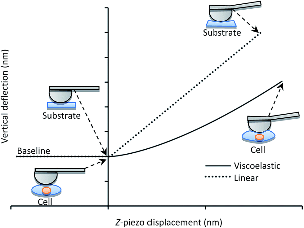 | ||
| Fig. 1 Cantilever vertical deflection versus z-piezo displacement during indentation of a single cell (solid line) and of an incompressible substrate (dotted line). | ||
These models derive from Hertz contact mechanics on the deformation of an elastic half-space indented by a conical shaped probe. They are used to extract Young's modulus values, which define the relationship between stress and strain (within the proportional/elastic region of a stress–strain curve) in a material. This mechanical property can be used to predict the behavior of a material upon elongation or compression. The effects of the probe's geometry are included by considering Sneddon's approximation.18,19 The resulting models encompass many assumptions including infinitesimal deformation, linearity of the half-space, infinite sample thickness, isotropic properties and flat (frictionless) contact surfaces. Additionally, they do not include parameters affecting the behavior of viscoelastic materials such as the loading rate. These assumptions do not perfectly reflect the characteristics of soft materials, but they may be, and have been, used nonetheless for comparative analyses to investigate variations in the viscoelastic properties of different samples in response to applied forces, given that the same type of probe and the same applied forces are used.20,21 The Hertzian model has actually been used in most of the literature to extract cells' Young's moduli in cases where indentation depth is much smaller than the probe radius and sample thickness.22–25
Current literature on the subject does not generally discuss the precise details of the experimental part and the data analysis procedure beyond what is usually provided in the Materials and methods section. Access to this information is crucial for researchers interested in reproducing the measurements of the elastic modulus of single cells, since minimal experimental variations may lead to different conclusions. To address this need, this report thoroughly outlines the experimental and analytical procedure to assess the elastic response of human NB4 acute promyelocytic leukemia (APL) derived white blood cells. APL is a serious type of leukemia that has transformed from highly fatal to highly curable.26,27 The initial intention of the work was to detect the elasticity values of NB4 cells at different stages and/or during drug treatments, which can provide insightful information not only in cancer research but also in additional health-related studies (e.g. cellular biomechanical response to nanostructured surfaces). However, we soon realized that optimized data collection and detailed step-by-step analysis process are critical and have not been reported extensively. Thus, the systematic procedures described in this paper will provide practical guidelines for researchers interested in quantifying cell elasticity.28,29
It should be noted that the AFM investigation of non-adherent cells such as NB4 cells is a challenging endeavor. In fact, imaging of cells usually requires chemical or biochemical immobilization to firmly fix them onto the substrate, a procedure that may however alter cell membrane structures and thus their mechanical properties. Therefore, in order to avoid these limitations, microwell arrays were used to physically confine NB4 cells for AFM indentation measurements.10 The photo-resistant material was patterned using soft lithography and the dimensions of the microwells were optimized to confine suspended cells while maintaining them within a reachable range of the AFM probe.
All experimental factors such as applied forces, force curve resolutions and loading rates, that can largely influence the determination of the elasticity values, were carefully considered and optimized in the data collection and fitting process. The development of an automated batch analysis code provides the possibility to fully understand the fitting models and obtain fast and consistent comparisons. It also permits identification of the appropriate criteria for cancer cell measurements. Such criteria include proper contact point location determination and identification of the maximum indentation length that should be fitted to avoid any substrate effect.
Materials and methods
Cell culture
The NB4 cell line, derived from human promyelocytic leukemia, was provided by Mount Sinai Hospital in Toronto (Dr Chen Wang). The cells were ordered from DSMZ (Deutsche Sammlung von Mikroorganismen Zellkulturen, Brauschweig, Germany, catalogue #: ACC-207). NB4 cells were cultured in Gibco® DMEM (Life Technologies, NY, USA), high glucose, with 10% of Gibco® heat-inactivated fetal calf serum (Life Technologies, NY, USA) and 1× of Gibco® penicillin (Life Technologies, NY, USA) in a humidified incubator (Sanyo North America Corp., IL, USA) containing 5% CO2, 95% humidity at 37 °C. Cells were passaged every 2–3 days to maintain a cell population of 105 cells per mL within 75 cm2 Corning™ Biocoat™ cell culture flasks (Fischer Scientific, PA, USA).Preparation of microwell arrays
Fig. 2 displays the step-by-step procedure to fabricate an SU8-10 microwell array substrate to mechanically confine APL cells. #1 glass coverslips were first cleaned in Piranha solution (mixture of 1![[thin space (1/6-em)]](https://www.rsc.org/images/entities/char_2009.gif) :4 of 30% H2O2 and 96% H2SO4), thoroughly rinsed with 18 MΩ cm Milli-Q H2O and finally dried in a nitrogen stream. (Caution: Piranha solution is a strong oxidant, reacts violently with organic materials and should be handled with utmost care). A clean coverslip was fixed in the spin coater (Laurell Technologies Corporation, PA, USA) before depositing 5 drops of SU8-10 photoresist solution (MicroChem, MA, USA). Spin coating at 3000 rpm for 65 s was performed according to the manufacturer's protocol to control well depth between 7 and 8 μm. Well depth was confirmed using a cyberSCAN CT 100 high resolution non-contact profilometer (Cyber Technologies, Eching-Dietersheim, Germany).
:4 of 30% H2O2 and 96% H2SO4), thoroughly rinsed with 18 MΩ cm Milli-Q H2O and finally dried in a nitrogen stream. (Caution: Piranha solution is a strong oxidant, reacts violently with organic materials and should be handled with utmost care). A clean coverslip was fixed in the spin coater (Laurell Technologies Corporation, PA, USA) before depositing 5 drops of SU8-10 photoresist solution (MicroChem, MA, USA). Spin coating at 3000 rpm for 65 s was performed according to the manufacturer's protocol to control well depth between 7 and 8 μm. Well depth was confirmed using a cyberSCAN CT 100 high resolution non-contact profilometer (Cyber Technologies, Eching-Dietersheim, Germany).
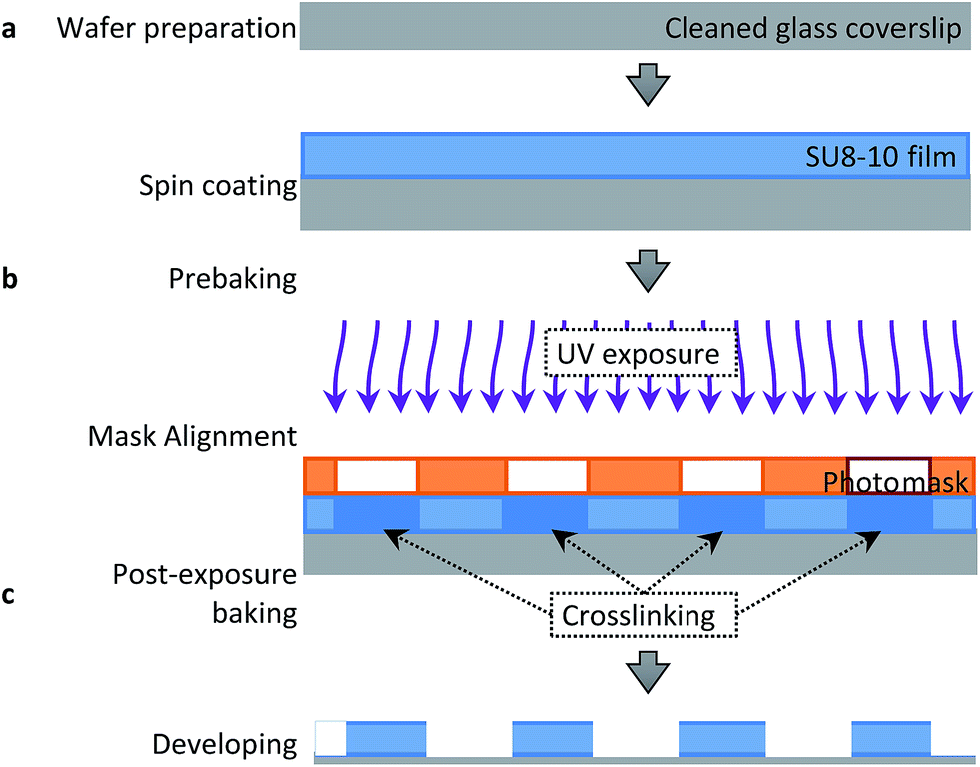 | ||
| Fig. 2 SU8-10 microwell arrays fabricated on glass coverslips by the soft lithography technique. SU8-10 was spin coated on a cleaned glass coverslip to obtain a uniform film (a). After prebaking the SU8-10 film was patterned using a photomask with an array of 20 μm circles inside the mask aligner undergoing UV exposure (b). After the post-exposure baking the non-crosslinked SU8-10 film areas were removed from the glass coverslip via immersion in the developer solution to generate an SU8-10 microwell array (c). | ||
Once the final spin coating procedure terminated, substrates were baked using heat blocks at 65 °C for 2 min followed by further baking at 95 °C for 5 min to evaporate the coating solvent and densify the coating after spin coating, respectively. The substrate was then placed in the mask aligner (Karl Suss America Inc., VT, USA) against a photomask (HTA Photomask, CA, USA) patterned by an array of 20 μm circles. Both the substrate and photomask were exposed to UV light for 12 s. Longer exposure time may result in backscattering and decompose development inhibitors away from the exposed film areas within the patterned circles. This may explain the sloping of the microwell walls seen in Fig. 3b of ±1 μm. Substrates were then post-exposure baked for 1 min at 65 °C and 2 min at 95 °C in order to remove standing wave ridges by diffusing the photoactive compound in the resist.
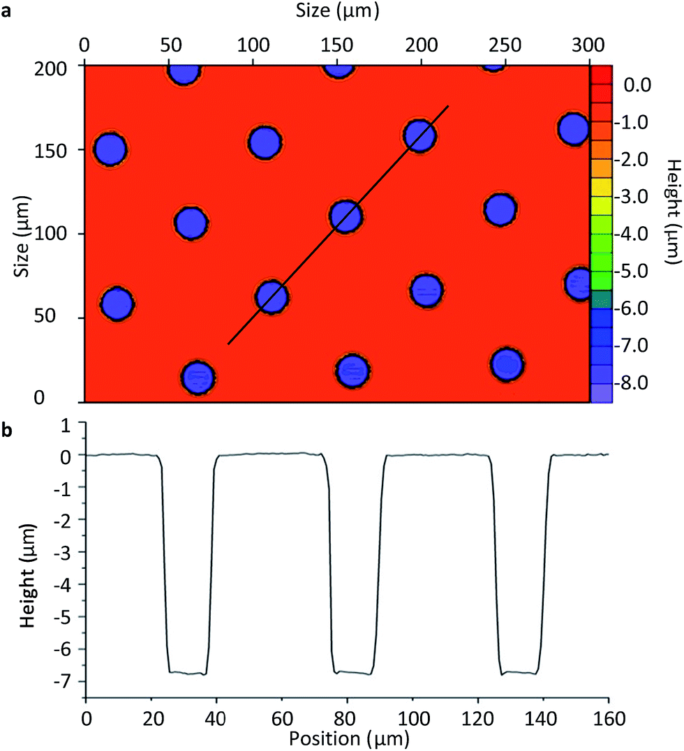 | ||
| Fig. 3 Non-contact profilometer image of the SU8-10 microwells (a) and the height profile of the microplate wells (b). | ||
Finally, the SU8-10 film on the coverslip (in short SU8-10 substrate) was left untouched overnight before immersion into the SU8 developer solution of 1-methoxy-2-propanol acetate (MicroChem, MA, USA) for 2 min, mixing gently every few seconds. Substrates were then rinsed with isopropanol and dried using a nitrogen stream, followed by baking at 35 °C for 1 to 2 h to harden the final SU8-10 film before final inspection. No major or minor cracks could be observed in the film by optical microscopy.
AFM measurements
Both the SU8-10 microwell substrate and AFM liquid cell were thoroughly rinsed using 70% ethanol and 18 MΩ cm Milli-Q H2O consecutively. The SU8-10 substrate was then placed at the bottom of a closed liquid cell (JPK Instruments CoverslipHolder, JPK Instruments, Berlin, Germany), which was successively filled with 800 μL of DMEM with 1× penicillin before placing it into a vacuum chamber. After vacuuming for 30 min, no air bubbles should be visible. It should be noted that no fetal bovine serum was used due to its viscosity which would cause formation of foam during vacuuming. The DMEM and penicillin solution was systematically replaced with 200 μL of warm culturing media at 37 °C, followed by the addition of 100 μL of cell solution in the liquid cell. The whole sample was placed on the AFM stage for 10 min before any further testing, to ensure the NB4 cells settled inside the microwells.Force-indentation curves were collected using a JPK Nanowizard® II BioAFM (JPK Instruments, Berlin, Germany) setup mounted on an inverted microscope (1X81, Olympus, Japan) with a manual precision stage (JPK Instruments, Berlin, Germany), under force mapping mode. Contact mode conical probes (DNP-10, Bruker AFM Probes, CA, USA) with a nominal spring constant of 0.06 N m−1 and colloidal probes (sQube®, Wetzlar, Germany) with a nominal cantilever spring constant of 0.08 N m−1 were used for the analysis of the conical (eqn (3)) and the spherical models (eqn (4)). Spring constants of each cantilever were individually determined by using the thermal noise method.30,31 The spring constants were measured in the 0.068–0.102 N m−1 range for conical and 0.047–0.071 N m−1 range for spherical probes, respectively.
Fig. 4 displays the schematic AFM setup for cell indentation measurements. The spherical probe attached to the AFM soft cantilever was used to indent the confined APL cells (pink). As shown, cell immobilization was achieved by using the fabricated patterned SU8-10 substrate, which is displayed as a bright field image on the top right of Fig. 4. The 20 μm microwells were sized to restrain the 15 to 20 μm cells.32–34 The 7 to 8 μm depth of the wells facilitates cell indentation by stably localizing cells inside the wells while maintaining a portion of the cell above the flat SU8-10 film surface.
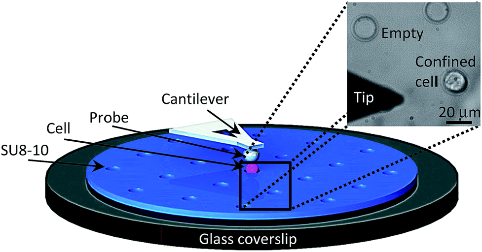 | ||
| Fig. 4 Main components of the experimental AFM setup to probe a single NB4 cell (pink) using a spherical tip (gray). The cell is confined within the patterned SU8-10 film microwell (blue) prepared over a glass coverslip wafer (black). A top view optical bright field image (top right) of the SU8-10 microwell array displaying empty microwells, a confined NB4 cell within a microwell as well as the AFM tip. | ||
Arrays of curves (vertical deflection versus z-piezo displacement) were collected over multiple (10 < n < 15) NB4 cells with selected grid sizes of 7 by 7, 15 by 15, 25 by 25, and 64 by 64 grids. Scan size was limited to 10 nm by 10 nm, in order to restrict lateral movement of the cantilever and constrain the probe motion above the cell surface. The procedure was repeated using both the conical and spherical probes. Only the approaching force curves collected for each grid were analyzed. A constant loading rate of 2 μm s−1 and a maximum load ranging from 0.5 nN to 2.0 nN were applied.7 From the cantilever spring constants and applied load range, the maximum deflection of the cantilever was between approximately 10 nm and 30 nm. The sampling rate was set to 2047 Hz in order to obtain over 3000 data points per curve for a z-scan length of 3 μm (maximum z-scan range is 15 μm). Extending and retracting delays were used (total of 0.2 s) to allow the NB4 cells to relax between consecutive indentations.
15 sets of deflection–displacement curves (49/225/625/4096 curves per set) were batch analyzed using a self-developed code implemented in IGOR Pro 6 (Wavemetrics, OR, USA). For each curve, the Young's modulus was extracted using respective equations and models (vide infra).
Fitting models
Two models using spherical and conical contact mechanics models were considered (Fig. S1†). In both models the following parameters derived from experiments were used for calculating the Young's modulus (E): the deflection (d), the ramp of the z-piezo (Z) and the cantilever's spring constant (k).The cantilever deflection as a function of the ramp can be converted to force (F) versus indentation (δ) by using eqn (1) and (2), in order to be fit to the desired models, i.e., eqn (3) and (4) (ref. 20 and 35–37) (eqn (1) and S(2)†). All data points on a given curve were fit to the appropriate models using the least square method. Each data point, i, of a deflection–displacement curve can be defined as (Zi, di) and the contact point being labeled by the index 0 (Z0, d0).
| F = kd = k(Z − δ) | (1) |
| δ = (Z − Z0) − (d − d0) | (2) |
In order to simplify the data processing and use only one fitting model, all data were processed two times using first the deflection versus ramp size curves, fit to eqn (3) and (4), and then the force-indentation curve, fit to eqn (1) and (2), for comparison purposes and validation.38 The Poisson ratio (v) was set to 0.5, as the material is assumed to be perfectly incompressible in order to simplify the model. In both models, information on the probe size and geometry is required, namely the opening angle (α) when using a conical probe and the radius (R) when using the spherical model.
Conical model:
 | (3) |
Spherical model:
 | (4) |
Automated data processing code
One of the challenges encountered during force data processing was to accurately fit over 50000 curves using self-defined criteria within a reasonable timeframe. An automated data processing code was thus necessary to enable the handling of large datasets comprising different formats including commercial AFM and ASCII files. The code also needed to include an extensive range of capabilities for scientific analysis such as the creation of user-defined curve fitting approaches and plotting of processed data. The details of the code design (Fig. S2†) and operation (Table S6†) can be found in the ESI.†
In addition, the code is also compatible with different text file layouts as different AFM instruments export the data curve in different formats. Thus, as both the JPK and DI (Bruker) software were available, the batch analysis code could be used for either formatting type. This is important to consider for users performing experiments on different AFM instruments.
Results and discussion
Optimization of the contact point location calculations
The accuracy of the contact point location (Z0, d0) will influence the fitting and thus the resulting Young's modulus. In order to achieve the optimal fitting to the selected models and extract comparable Young's modulus values, one of the first steps in the automated processing is to identify the location of the contact point (Z0, d0).As shown in Fig. 5, two reference points, (Z1, d1) and (Z2, d2), were selected on the deflection curve. (Z1, d1) was chosen in order to best represent the cell behavior upon small deflection, i.e., closer to 0% of the deflection, meanwhile (Z2, d2) represents the larger deflection portion, i.e., closer to 100% of the deflection. It is noteworthy to emphasize that neither point is chosen within the baseline region, which should not be fit as it does not represent any contact between the tip and sample. When offsetting the deflection to the point at which the probe and cell were in contact (d0 = 0), the contact point finding eqn (5) became38
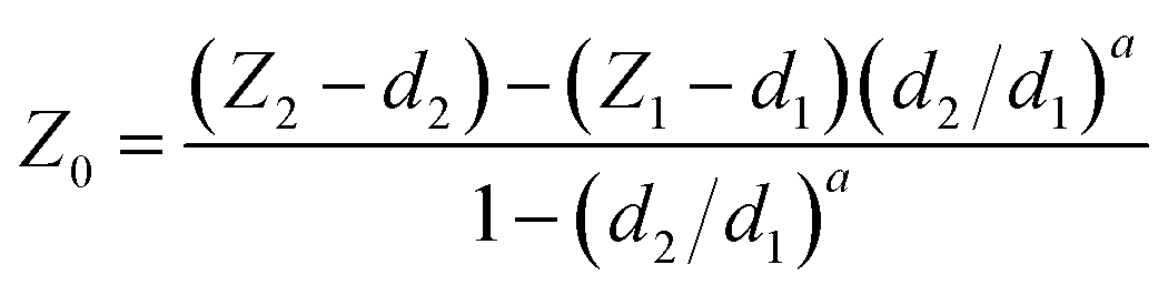 | (5) |
 | ||
| Fig. 5 Reference points (Z1, d1) and (Z2, d2) located between 0% and 100% of the deflection, used to determine the contact point (Z0, d0) on an experimentally captured deflection–displacement curve. | ||
By systematically offsetting the deflection d0 to zero, the contact point can be recalculated until its location remains constant or within a given range (e.g., 0 to 25 nm). Fig. 5 represents an experimental deflection–displacement curve for which a maximum applied force of about 0.5 nN was used (the cantilever spring constant was 0.059 N m−1). This gave the maximum deflection of the cantilever to approximately 10 nm. The z-piezo displacement length was set to 3 μm (measured between 11 and 8 μm in Fig. 5, within the total z-scan range of 15 μm).
In principle, for an ideal curve where the relationship between deflection (or force) and displacement (or indentation) perfectly matches the model, regardless of which two points (Z1, d1) and (Z2, d2) are selected, it would result in the same contact point location. In reality, with different noise levels and non-ideal correlations, the contact point may vary when choosing different (Z1, d1) and (Z2, d2). Thus, how to select the location of (Z1, d1) and (Z2, d2) is critical for determining the contact point location. Here, systematic pairing comparisons were evaluated by selecting these points based on the percentage of the deflection, setting the largest deflection at 100%, and the baseline of deflection being 0%. The analyzed results are shown in Tables 1 and S1.†
| (Z1, d1) (% curve) | (Z2, d2) (% curve) | Ratio of the average variation of the fitting errora (±SD ratio) | Ratio of the average variation of the indentation lengtha (±SD ratio) | Ratio of the average variation of the number of data pointsa (±SD ratio) | Ratio of the average variation of the Z0 locationa (nm ± SD ratio) |
|---|---|---|---|---|---|
a
 . .
|
|||||
| 25 | 1.16 ± 0.39 | 1.13 ± 0.34 | 1.14 ± 0.36 | 1.01 ± 0.08 | |
| 50 | 1.05 ± 0.34 | 1.01 ± 0.24 | 1.01 ± 0.25 | 1.00 ± 0.07 | |
| 10 | 60 | 1.00 ± 0.33 | 1.00 ± 0.26 | 1.00 ± 0.27 | 1.00 ± 0.07 |
| 75 | 0.97 ± 0.34 | 0.97 ± 0.27 | 0.97 ± 0.27 | 1.00 ± 0.06 | |
| 90 | 0.95 ± 0.32 | 0.96 ± 0.25 | 0.95 ± 0.25 | 0.99 ± 0.06 | |
| 25 | 1.09 ± 0.46 | 1.10 ± 0.36 | 1.12 ± 0.39 | 1.01 ± 0.08 | |
| 50 | 0.99 ± 0.36 | 0.99 ± 0.27 | 0.99 ± 0.28 | 1.00 ± 0.07 | |
| 15 | 60 | 0.95 ± 0.35 | 0.98 ± 0.27 | 0.98 ± 0.29 | 1.00 ± 0.06 |
| 75 | 0.92 ± 0.38 | 0.94 ± 0.29 | 0.93 ± 0.30 | 0.99 ± 0.06 | |
| 90 | 0.89 ± 0.35 | 0.91 ± 0.27 | 0.91 ± 0.27 | 0.99 ± 0.06 | |
Before selecting the two points, some general rules should be applied: (1) (Z1, d1) should not be located below 10%, in order for the code to have sufficient data points (prior to the contact point) to separate the baseline data points from the deflected data points; (2) (Z2, d2) should not be selected below 50%, in order to avoid representing only the shallow indentation portion of the deflection–displacement curve which may cause eqn (5) to misinterpret the location of the contact point; (3) when selecting (Z1, d1) to be above 20% of the deflection, the lower deflection regime is not fully taken into account in the contact point eqn (5) and may cause a misapprehension of the contact point location. Therefore, (Z1, d1) should be selected between 10 and 20%.
Table S1† gives the absolute values for all contact point locations from different applied loads. However, Table 1 focuses on the relative results using a 0.5 nN applied force only with the chosen reference points ((Z1, d1) and (Z2, d2)) selected at 10% and 60% of the deflection. It is an overview of the absolute values of the contact point location results shown in Table S1† when selecting different reference points.
When choosing the reference point (Z2, d2) at a location lower than 50% of deflection, although the contact point did not fluctuate much, an increase not only in the fitting error (eqn S3†) but also in the indentation length (calculated from the deflection and z-piezo displacement as described in the ESI†) and number of fitted data points was also observed. Additionally, in most calculations the coefficients of variation increased as well. The most dramatic increase in data variation was found when the (Z2, d2) reference was located below 25% of the maximum deflection curve. When selecting a (Z2, d2) above 50%, results did not display drastic changes. As coefficients of variation were lower for almost every factor, (Z2, d2) above 50% was identified as a workable reference to locate the contact point. However, reference (Z2, d2) should be carefully assessed for cases in which large applied loads are used, as the fittings may be influenced by substrate effects recorded by the deflection curves.
On comparing the results, locating the contact point by using the deflection at 15% instead of 10% for the reference point (Z1, d1), the coefficient of variation was similar. However, when using both 15% and 25% as reference points, a smaller portion of the force curve was represented, generating a larger increase in the fitting analysis results and in the data variability.
Fig. 6 displays the contact point location (Z0, d0) and Young's modulus dependency of the reference points used to locate it. For each of the 49 deflection curves collected using a 0.5 nN applied force, the contact point was calculated by selecting three different pairs of (Z1, d1) and (Z2, d2) references at deflection positions of 10% and 25% (black), 10% and 60% (red) and 10% and 90% (green), to verify the consistency of the calculated contact point location, respectively. 88% (43 curves out of 49) of the calculated contact point locations and Young's modulus values were different, while 12% (6 curves) were consistent. The three paired positions (Z1, d1) and (Z2, d2) as references to the contact point location (eqn (5)) showed the influence and importance of these reference points (Fig. 6a). Young's modulus measurements using these same criteria are displayed in Fig. 6b. Consistent contact point locations (i.e., calculated contact points overlay), such as in curves #0, #5, #26, #32, #34, #36 and #49 (Fig. 6a), resulted in consistency of the Young's modulus measurements (Fig. 6b). When selecting 10% (d1) and 25% (d2), outliers such as in curves #18, #19, #23, #38 and #39 were observed (Fig. 6a). This correlated with outliers of the measured Young's modulus values (Fig. 6b).
 | ||
| Fig. 6 Contact point locations (a) and Young's modulus values (b) obtained by fitting the deflection-z-piezo displacement curves to the spherical model using different reference points (Z1, d1) and (Z2, d2) at 10% and 25% (black), 10% and 60% (red) and 10% and 90% (green) of the deflection. Total curves n = 49 and 0.5 nN applied force were analyzed. | ||
Although contact point location was observed to increase throughout the 49 indentations of the NB4 cell (Fig. 6a), this was likely due to the drift of the tip since the Young's modulus measurements were independent of that trend. When choosing the two reference points at deflections of 10% and 25%, only the beginning of the curves may comply with the models. Too many points on the curve were ignored, representing only a small indentation and superficial tip-sample contact. This information could not be easily seen in Tables 1 and S1† due to the large absolute value of the contact point locations between −9500 nm and −7000 nm within the z-piezo displacement range. Hence, the coefficient of variation was calculated between 0.06 and 0.08 for the contact point location.
Most of the data calculated using reference points at 10% and 60% (red), as well as at 10% and 90% (green) were more consistent with each other and did not display as deviated as observed in the 10% and 25% dataset (black), when using an applied force of 0.5 nN (similar fitting information can be found in Tables S2 and S3† when using applied forces of 1.0 nN and 2.0 nN). When cells are indented using larger applied forces, substrate effects may become more obvious and (Z2, d2) should be positioned earlier on the deflection curve such as at 50% of the whole curve and not above 90%.
Finally, it is important to properly assess reference points used to locate the contact point as they not only influence the contact point location (eqn (5)), but also the fit Young's modulus values. Consistency in these reference point locations in terms of deflection percentage is crucial and should be standardized according to the specific AFM parameters used. In most of the NB4 cell indentation measurements, we choose to use 10% and 60% as the reference points to locate the contact point positions.
Comparison of the fitting models
As previously mentioned, two fitting models were considered in the indentation measurements for calculating the Young's modulus. Multiple force indentation measurements were performed using different conical and spherical probes. Fitting values of Young's modulus were compared using the two modules.Fig. 7 displays the fit Young's modulus values using 250 force curves measured on NB4 cells. An applied force of 0.5 nN was used for both a conical probe and a spherical probe (20 μm in diameter) over different NB4 cells. Histograms represented the Young's modulus distributions when using either spherical or conical probes and fit to the respective models, namely eqn (3) for the conical probe and eqn (4) for the spherical probe (ESI†). When using a conical probe and eqn (3), a wider data distribution between 0.266 and 6.280 kPa was observed, when compared to the narrower distribution of 0.025 to 0.248 kPa when using a spherical probe and eqn (4). For the 250 force curves, average Young's moduli of 1.309 ± 0.805 kPa and 0.095 ± 0.039 kPa were calculated using a conical probe and a spherical probe, respectively. The larger Young's moduli measured using the conical probe is expected from the larger indentation of the cell required to reach a 0.5 nN indentation force. However, discrepancy can be observed in both models. It may not only be explained by the viscoelastic behavior of the cell which is not taken into account in these models but also from the fact that the measurements are taken on a dynamic system. At the nanoscale, media flow and other cellular components (apoptotic bodies or cells) may introduce artifacts in the indentation measurements.
 | ||
| Fig. 7 Representative Young's modulus values obtained from 250 deflection–displacement curves measured on individual NB4 cells under an applied load of 0.5 nN, using a conical and a spherical probe. Data were fit to the respective models (eqn (3) and (4)). Inset: scattered plots of the Young's moduli for both probe types with respect to the curve number. | ||
The inset in Fig. 7 shows a scattered plot of the Young's modulus values obtained from 250 consecutive deflection–displacement curves for both probes. The inset displays the same dataset plotted in the histograms. It represents the data variability when using a conical or spherical probe. It was found that the data using the conical probe resulted in a greater amount of outliers. However, when comparing the standard deviation to the average Young's modulus values (coefficient of variation as shown in eqn S4†) for both the conical and spherical models, results were comparable (Fig. 7, inset). The relatively sharper probes (and fitting to the conical model, eqn (3)) may permit detection of local variations in elasticity on cell membranes instead of average elasticity with larger contact area when using a colloidal probe.
In this context, it has been hypothesized that the data collected using a conical probe can be fit to the spherical model.35 However, when fitting the data measured using a conical shaped probe to the spherical model with a probe radius of 50 nm, the same scattering was found in the plotted histograms, only the Young's modulus distribution was shifted to higher values. Fitting errors were higher when fitting the raw data with the inappropriate model. This indicates that when a conical probe is used to investigate the cells, a larger amount of data is required to properly represent the average elasticity of the cell membrane. The larger Young's modulus when using a conical probe can also be explained by the larger stress and strain concentrations exerted on the cell than that when using a spherical probe, when comparing data using the same applied load as it is closely related to the Young's modulus.39,40 This is not the case when fitting the data by controlling the indentation length, but the indentation length is not the parameter we wish to control during data collection.
By plotting the Young's modulus as a function of time (or curve number), as demonstrated in the inset of Fig. 7, it is possible to determine its variation from the collected data. The 250 consecutive curves measured using the spherical probe showed a consistent Young's modulus, thereby indicating that using the 20 μm colloidal probes and fitting data to the spherical model provide uniform elasticity measurements. The conical model seemed, on the other hand, to provide a larger scattering of the data, suggesting less reliable elasticity measurements. However, by considering the coefficient of variation of the data (using eqn S4†), conical (Cv = 0.615) and spherical (Cv = 0.413) data are similar (Fig. 7, inset). As the absolute values of the Young's modulus are required for comparability and small mechanical property alterations are necessary to evaluate different types of cancer cells at different stages (or subjected to different treatments), the spherical probes and spherical model were considered to properly determine the average elasticity of APL-NB4 cells.
The inset in Fig. 7 also helped identify cells that were influenced by their environment according to the magnitude of the differences in the elasticity values. This type of time-dependent Young's modulus measurements can also describe whether the cell has had sufficient time to relax between each tip-sample interaction by observing any time-dependent stiffening.5 However, this is not the case in Fig. 7, which included 250 force curves (13.33 min AFM collecting time, 0.5 nN applied force) using either model.
Lastly, the spherical probe was found to best represent average elasticity measurements of the NB4 cells, as it involves a larger tip-sample contact area and retrieves a narrower variability of the data. The conical probe also provides valid information of the cellular Young's modulus but its sharper shape may be associated with a greater penetration when applying the same load, which in turn may cause indentation of underlying organelles. For this reason, when using a conical probe, a larger number of deflection curves are required to properly represent the cell elasticity and observe any alteration of cell mechanics over time.
Assessment of cell tolerance to externally applied forces
Fig. 8 shows the assessment of the elasticity when indenting different NB4 cells with the conical and the spherical probes using different applied loads. Each box plot represents collected data from a single cell probed 49 times. Five different cells were considered to evaluate each applied load. For the assessment of each probe, 3 different conditions were considered, namely applied loads/forces of 0.5, 1.0, and 2.0 nN. All fittings were performed by fixing (Z1, d1) and (Z2, d2) at 10% and 60% of the deflection with respect to the whole curve, in order to locate the contact points (Table S4†).
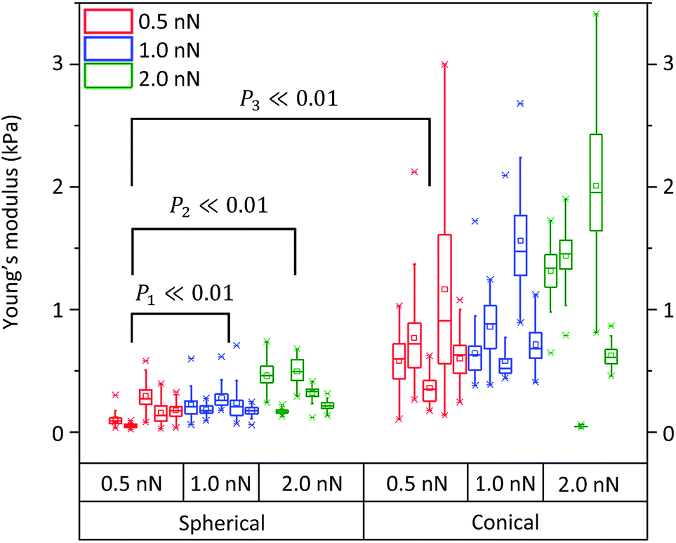 | ||
| Fig. 8 Elasticity measurements on 5 different NB4 cells for each assessed applied forces of 0.5 nN, 1.0 nN and 2.0 nN, respectively, using both a spherical probe and a conical probe. Young's modulus values were obtained by fitting 49 deflection–displacement curves to the respective models. Average (mean) Young's modulus values for single NB4 cells are labeled by square points within each box plot. Labeled values, calculated from a two-sample t-test are displayed. | ||
When considering the applied forces for cells probed with the spherical indenter, elasticity values increased upon raising the applied force to 2.0 nN. In particular, upon increasing the applied load from 0.5 nN to 1.0 nN and 2.0 nN, a mean Young's modulus of 0.16 ± 0.07 kPa was obtained for an applied load of 0.5 nN, which increased to 0.22 ± 0.08 kPa and 0.34 ± 0.06 kPa at 1.0 nN and 2.0 nN, respectively. The same trend was observed with a conical probe when using the same load increments. However, unlike the previous case, changes were also observed between 0.5 nN and 1.0 nN. In fact, with a 0.5 nN force, the average elasticity was 0.70 ± 0.34 kPa, 0.87 ± 0.25 kPa for 1.0 nN, and 1.09 ± 0.22 kPa for 2.0 nN (conical probe, eqn (3), in Table S4†). Therefore, in agreement with results shown in Fig. 7 and 8, measurements using a conical probe (fitting to the conical model) might be associated with larger and more scattered Young's modulus values than those obtained with the spherical model (using 20 μm spherical probes). Such large variability in Young's modulus measurements may be explained by considering the probe's larger sensitivity to underlying organelles due to the concentrated stress exerted by conical tips. In fact, smaller applied forces are required to indent the smaller depth of the cell membrane when using a sharper probe. Cells thus appear to better tolerate the indentation of a large sized spherical probe, rather than that of a sharper conical probe.
A two-sample t-test revealed that the mean Young's modulus values are significantly different (P ≪ 0.01) when using these different applied forces with either conical or spherical probes. In Fig. 8, all data between groups (spherical and conical models) or subgroups (0.5, 1.0 and 2.0 nN applied forces) were significantly different. In addition, as expected, when comparing the 0.5 nN applied force to the 1.0 nN applied force within the spherical probe group, the probability of having similar groups was larger than when comparing the 0.5 nN subgroup to the 2.0 nN subgroup. Moreover, due to the variability in the conical probe data, 0.5 nN applied force between the spherical and the conical groups, the calculated probability was slightly lower than when comparing the 0.5 nN force and 2.0 nN within the spherical groups (P3 < P1 < P2 ≪ 0.01).
Fig. 9 displays the representative Young's modulus dependency of the fit indentation length. 49 force curves were consecutively collected using a 0.5 nN applied load over a single NB4 cell by 20 μm spherical probes. Curve fittings were performed to fit the deflection–displacement data to the spherical model. All 49 curves were fit by restricting the indentation length to different values, all starting from the calculated contact point located using reference points at 10% (Z1, d1) and 60% (Z2, d2). Six different Young's modulus values were calculated for each force curve using fit apparent indentation lengths of 200 nm, 400 nm, 600 nm, 800 nm, 1000 nm and the full indentation length. Data are displayed in Table S5.†
 | ||
| Fig. 9 Young's modulus dependency of the fit indentation length of 49 force curves measured consecutively over a single NB4 cell using an applied load of 0.5 nN and spherical probe and model. Young's modulus values plotted as a function of curve number (a), indentation length (b), and fit to different indentation lengths with two representative force curves (an ideal curve, number 37 (c), and non-ideal curve, number 44 (d)). | ||
When different indentation lengths were selected to fit the same force curve, the Young's modulus varied accordingly. Fig. 9a presents the Young's modulus as a function of the curve number using different indentation lengths. On the other hand, Fig. 9b displays the Young's modulus as a function of indentation length alone, also showing the change and spreading levels in data variability when fitting the same curves (as in Fig. 9a) using different indentation lengths. When fitting the curves by setting the apparent indentation to 200 nm and 600 nm, the mean Young's modulus values were 0.164 ± 0.106 kPa, and 0.103 ± 0.054 kPa, respectively. As shown in Fig. 9b, spreading of the data was also found to be larger using a 200 nm indentation length. When performing two-sample t-tests with respect to the full indentation length of the deflection curves, only the apparent indentation length of 200 nm was revealed to significantly differ from the fittings performed using the full deflection curve (P ≪ 0.01).
Fig. 9c and d represent individual deflection-z-piezo displacement curves that were fit using the different indentation lengths. Curve #37 (Fig. 9c) demonstrates the ideal smooth curve which obeyed the fitting model quite well. When increasing the apparent indentation length from 200 to 1000 nm, Young's modulus values varied from 0.11 to 0.08 kPa. However, in the case of a non-ideal curve, such as in Fig. 9d, fittings using similar apparent indentation lengths (200 to 1000 nm) resulted in a decrease of the Young's modulus from 0.68 kPa to 0.09 kPa. This clearly shows the importance of controlling the appropriate indentation parameters during data collection to avoid variation of the fitting results.
It should be noted that in both Fig. 9a and b, when the full indentation length of the curve ranged below the selected apparent indentation length, the full indentation length was used to fit the curve. For example, a curve with an indentation length of 500 nm would be fit to 500 nm for a selected 600, 800 or 1000 nm as apparent indentation. This occurrence was observed in Fig. 9b when the Young's modulus values were repeated for indentation lengths other than those selected (i.e., other than 200, 400, 600, 800, 1000 nm). In other words, when the maximum indentation length was set to a value smaller than that of the whole curve, the entire force curve was fit, causing false overlays of the fitted data (Fig. 9a and b). For example, curve #12 involves identical Young's modulus measurements of 0.249 kPa when using an indentation length of 600 nm and higher as the indentation length of the whole curve was 559.92 nm (Fig. 9a and b).
Finally, a minimum indentation length of 600 nm should be considered to avoid scattering of the data and avoid the influence of shallow contact or keep the contact area as consistent as possible during data collection. It is important to understand that when substrate effects need to be avoided, limiting the indentation length during fittings to correct the use of a large applied force is not a solution. When using a small force such as 0.5 nN, the whole curve should be fit in order to maintain consistent and comparable fittings. This avoids biased elasticity measurements and is an important factor to consider when collecting force curves. AFM parameters should not be altered for fitting purposes after data collection, in order to maintain a consistent applied force between indentations. Maximum applied load and scan length should be optimized prior to data analysis, to avoid misleading results.
Conclusions
In order to complement the existing literature, we have developed an automated batch analysis code to perform unbiased data processes on AFM indentation data measured over leukemia cancer cells. Both AFM experimental parameters such as probe selection and maximum applied force, as well as fitting criteria including contact point location and indentation lengths, were optimized and reported in this study.By confining the non-adherent NB4 cells into SU8-10 microwell arrays, it was possible to systematically study the mechanical properties of these cells by AFM based force indentation measurements. A significant amount of raw data was collected, in order to provide reference elasticity values for NB4 cells. Applied forces and indentation lengths, the measurement velocity and substrate treatments were found to be important parameters before and during data compilation. Additional criteria, such as the location of the contact point and the selection of adequate contact mechanics models, were essential to properly fit the indentation portion of the force curves. Thus, several fitting criteria were defined to best optimize data processing and obtain consistent and comparable results. The contact point location was reliably found by using the two-reference-point approach, (Z1, d1) and (Z2, d2), at 10% and 60% of the deflection, respectively. Although both conical and spherical models were studied, the spherical probe was found to be more appropriate for the APL cancer cell detection by better representing the average Young's modulus, with narrow distributions. Furthermore, a range of applied forces and cell indentation lengths were assessed, in order to improve force curve collections over NB4 cells by identifying applied load magnitudes that reduce cell damage, substrate effects, as well as shallow indentation.
The outcome of understanding and perfecting this analysis protocol contributed to obtaining various comparative cell mechanics results. By indenting the NB4 cells with a 2 nN force, Young's modulus was found to be twice as large as the elasticity measurements when using a 0.5 nN force. When using a smaller force such as 0.5 nN to extract the Young's modulus of NB4 cells, full indentation lengths were used to fit the deflection–displacement curves. More adjustments may be carried out to the code in order to increase its speed and accuracy. After reproducing more consistent results on untreated NB4 cell lines, future work using the optimized experimental conditions and parameters determined in this study will involve the monitoring of NB4 cell line elasticity changes when treated with different drugs. Such assessment will show the potential of cell elasticity measurements using AFM as a drug screening and cancer staging tool. Future work should aim on the customization of the Hertzian model so that it may include the viscoelastic properties of biological samples in order to best represent the data and create a comparable database for different cell types.
Acknowledgements
The authors thank the financial support provided by the National Research Council of Canada (NRC) and the Natural Sciences and Engineering Research Council (NSERC) of Canada. HF and SZ thank Dr Maohui Chen for the help in SU8-10 substrate preparation.References
- S. E. Cross, Y.-S. Jin, J. Rao and J. K. Gimzewski, Nat. Nanotechnol., 2007, 2, 780–783 CrossRef CAS PubMed.
- H. Huang, R. D. Kamm and R. T. Lee, Am. J. Physiol.: Cell Physiol., 2004, 287, C1–C11 CrossRef CAS PubMed.
- Q. S. Li, G. Y. H. Lee, C. N. Ong and C. T. Lim, Biochem. Biophys. Res. Commun., 2008, 374, 609–613 CrossRef CAS PubMed.
- N. Walter, T. Busch, T. Seufferlein and J. P. Spatz, Biointerphases, 2011, 6, 79–85 CrossRef CAS PubMed.
- O. Chaudhuri, S. T. Koshy, C. Branco da Cunha, J.-W. Shin, C. S. Verbeke, K. H. Allison and D. J. Mooney, Nat. Mater., 2014, 13, 970–978 CrossRef CAS PubMed.
- S. Suresh, Acta Biomater., 2007, 3, 413–438 CrossRef PubMed.
- M. T. Frey, A. Engler, D. E. Discher, J. Lee and Y.-L. Wang, Methods Cell Biol., 2007, 83, 47–65 CAS.
- J. P. Mills, L. Qie, M. Dao, C. T. Lim and S. Suresh, Mech. Chem. Biosystems, 2004, 1, 169–180 CAS.
- A. M. Powe, S. Das, M. Lowry, B. El-Zahab, S. O. Fakayode, M. L. Geng, G. A. Baker, L. Wang, M. E. McCarroll, G. Patonay, M. Li, M. Aljarrah, S. Neal and I. M. Warner, Anal. Chem., 2010, 82, 4865–4894 CrossRef CAS PubMed.
- M. J. Rosenbluth, W. A. Lam and D. A. Fletcher, Biophys. J., 2006, 90, 2994–3003 CrossRef CAS PubMed.
- J. K. Li, R. M. A. Sullan and S. Zou, Langmuir, 2011, 27, 1308–1313 CrossRef CAS PubMed.
- T. G. Kuznetsova, M. N. Starodubtseva, N. I. Yegorenkov, S. A. Chizhik and R. I. Zhdanov, Micron, 2007, 38, 824–833 CrossRef CAS PubMed.
- Z. Deng, V. Lulevich, F. Liu and G. Liu, J. Phys. Chem. B, 2010, 114, 5971–5982 CrossRef CAS PubMed.
- D. Kirmizis and S. Logothetidis, Int. J. Nanomed., 2010, 5, 137–145 CrossRef.
- V. Lulevich, T. Zink, H.-Y. Chen, F.-T. Liu and G. Liu, Langmuir, 2006, 22, 8151–8155 CrossRef CAS PubMed.
- M. E. Dokukin and I. Sokolov, Langmuir, 2012, 28, 16060–16071 CrossRef CAS PubMed.
- J. Seifert, J. Rheinlaender, P. Novak, Y. E. Korchev and T. E. Schäffer, Langmuir, 2015, 31, 6807–6813 CrossRef CAS PubMed.
- A. C. Fischer-Cripps, Introduction to Contact Mechanics, Springer US, Boston, MA, 2nd edn, 2007 Search PubMed.
- K. L. Johnson, Contact Mechanics, Cambridge Univ. Press, Cambridge, 9th edn, 2003 Search PubMed.
- D. C. Lin, E. K. Dimitriadis and F. Horkay, J. Biomech. Eng., 2007, 129, 430–440 CrossRef PubMed.
- N. Guz, M. Dokukin, V. Kalaparthi and I. Sokolov, Biophys. J., 2014, 107, 564–575 CrossRef CAS PubMed.
- M. Lekka and P. Laidler, Nat. Nanotechnol., 2009, 4, 72 CrossRef CAS PubMed.
- J. R. Staunton, B. L. Doss, S. Lindsay and R. Ros, Sci. Rep., 2016, 6, 19686 CrossRef CAS PubMed.
- M. Glaubitz, N. Medvedev, D. Pussak, L. Hartmann, S. Schmidt, C. A. Helm and M. Delcea, Soft Matter, 2014, 10, 6732–6741 RSC.
- G. Thomas, N. A. Burnham, T. A. Camesano and Q. Wen, J. Visualized Exp., 2013, 76, e50497 Search PubMed.
- Z.-Y. Wang and Z. Chen, Blood, 2008, 111, 2505–2515 CrossRef CAS PubMed.
- W. A. Lam, M. J. Rosenbluth and D. A. Fletcher, Blood, 2007, 109, 3505–3508 CrossRef CAS PubMed.
- F. Lautenschläger, S. Paschke, S. Schinkinger, A. Bruel, M. Beil and J. Guck, Proc. Natl. Acad. Sci. U. S. A., 2009, 106, 15696–15701 CrossRef PubMed.
- A. Gaman, E. Osiac, I. Rotaru and C. Taisescu, Curr. Health Sci. J., 2013, 39, 45–47 Search PubMed.
- J. L. Hutter and J. Bechhoefer, Rev. Sci. Instrum., 1993, 64, 1868–1873 CrossRef CAS.
- J. Lübbe, M. Temmen, P. Rahe, A. Kühnle and M. Reichling, Beilstein J. Nanotechnol., 2013, 4, 227–233 CrossRef PubMed.
- B. Ciesla, Hematology in Practice, 2011, 131 Search PubMed.
- K. D. McClatchey, Clinical Laboratory Medicine, Lippincott Williams & Wilkins, 2002 Search PubMed.
- P. Murphy, The Neutrophil, Springer Science & Business Media, 2012 Search PubMed.
- C. A. Grattoni, H. H. Al-Sharji, C. Yang, A. H. Muggeridge and R. W. Zimmerman, J. Colloid Interface Sci., 2001, 240, 601–607 CrossRef CAS PubMed.
- S. Sen, S. Subramanian and D. E. Discher, Biophys. J., 2005, 89, 3203–3213 CrossRef CAS PubMed.
- D. Lee, M. M. Rahman, Y. Zhou and S. Ryu, Langmuir, 2015, 31, 9684–9693 CrossRef CAS PubMed.
- J. A. Last, S. J. Liliensiek, P. F. Nealey and C. J. Murphy, J. Struct. Biol., 2009, 167, 19–24 CrossRef CAS PubMed.
- L. Ma, L. Levine, R. Dixson, D. Smith and D. Bahr, in Nanoindentation in Materials Science, ed. J. Nemecek, InTech, 2012, 35 Search PubMed.
- E. K. Dimitriadis, F. Horkay, J. Maresca, B. Kachar and R. S. Chadwick, Biophys. J., 2002, 82, 2798–2810 CrossRef CAS PubMed.
Footnote |
| † Electronic supplementary information (ESI) available: Fitting models, detailed results with different criteria, and the design and performance of the code. See DOI: 10.1039/c6ay00131a |
| This journal is © The Royal Society of Chemistry 2016 |