
Three-dimensional hydrodynamic focusing microfluidic emitter: a strategy to inhibit sample ion expansion in nanoelectrospray ionization†
Bo
Xiong
*,
Lingling
Wang
,
Yujiao
Wang
,
Yajing
Bao
,
Shichang
Jiang
and
Mingyue
Ye
Key Laboratory of Pesticides & Chemical Biology, Ministry of Education, College of Chemistry, Central China Normal University, Wuhan 430079, P. R. China. E-mail: bx@mail.ccnu.edu.cn; Fax: +86-27-67867961; Tel: +86-27-67867961
First published on 27th November 2015
Abstract
A microfluidic emitter based on three-dimensional hydrodynamic focusing was developed to generate a wrapped charged aerosol plume, in which the distribution of the sample ion in the nanoelectrospray could be regulated. Deposition patterns of the wrapped spray from the proposed three-dimensional hydrodynamic focusing nanoelectrospray emitter (3D HFNE) were collected under different conditions to ensure the wrapped configuration. Moreover, sample ion intensities as well as their ratios to a focusing background ion were studied as a function of different displacements from the center of the wrapped electrospray to confirm the inhibition of ion expansion. Furthermore, the proposed 3D HFNE indicated improved sensitivities compared with a reported nanoelectropray emitter as well as its commercial ESI counterpart, and this demonstrated its capacity for determining samples with low concentrations and infusion rates. In addition, the proposed 3D HFNE was compatible with various sample flow compositions (from 100% methanol to 100% water) and a broad infusion rate range (from 10 nL min−1 to 15 μL min−1). Finally, its stability and durability were indicated to be acceptable for various determinations. Therefore, the 3D HFNE is a potential option to achieve on-line nanoelectrospray MS determinations using microfluidics with conventional mass spectrometers, considering its low cost and user-friendly properties.
Introduction
Microfluidic devices have indicated pronounced advantages in high throughputs,1,2 with low sample consumptions,3 as well as in feasible manipulations for single cells,4 and they have been widely applied in proteomics,3 single cell analysis,4–6etc. Meanwhile, nanoelectrospray ionization mass spectrometry (nanoESI-MS) has shown advantages in providing structural information compared with other microfluidic detection methods, e.g., fluorescence and electrochemical detections. Moreover, it is compatible with conventional infusion rates in microfluidics.7,8 Therefore, on-line strategies to couple microfluidic devices and nanoESI-MS have attracted broad interest.2,9–13One straightforward approach to achieve their combination was to integrate monolithic nanoESI emitters in microfluidic devices.14–16 These emitters were prepared during the fabrication of chips, and they conventionally had improved reproducibility and dead volumes compared with external emitters,17,18e.g., commercial nanoESI tips. However, monolithic microfluidic device-nanoESI-MS strategies have generally failed to be widely employed. One reason for this may be due to the difficulty of preparing reliable nanoESI interfaces in various chips.10,11
Firstly, a perfect substrate material for monolithic microfluidic nanoESI emitters was still absent. Various materials, including glass,17,19 SU-8,20 polyimide21 and polydimethylsiloxane (PDMS),22–24 have been used to fabricate integrated ESI emitters. Besides the difficulty of preparing glass emitters,17 which were all in specific shapes,25 the hydrophilic surface of the glass would negatively influence the stability of the electrospray.16,26 On the contrary, PDMS is hydrophobic, and its surface would distinctly reduce the wetting of the solution jetted out from the ESI tip.24 Moreover, it has been widely used in microfluidic fabrications. In this sense, PDMS-based nanoESI emitters, as interfaces to couple reported microfluidic devices with MS, would be of potential value. Smith and co-workers reported a PDMS membrane-based emitter,23 which was compatible with broad compositions of solvents, while the membrane thickness and various parameters for microfluidic channels were confined.
In addition, strict restrictions in shapes and configurations further increased the difficulty of preparing monolithic nanoESI emitters. Electrosprays tended to form at the microdefects on emitters,27 and this feature would limit their ionization efficiencies. Therefore, nanoESI emitters were conventionally made in sharpened shapes to ensure their performances.28 Moreover, the feasibility of preparing nanoelectrosprays using conventional nanoESI emitters mainly depended on their capacities to generate small droplets with low infusion rates. Therefore, it was broadly chosen to prepare microchannels with comparably limited sizes or specific configurations.1,13,19,28–30 Unfortunately, these nozzles would be more prone to clogging compared with their conventional counterparts, and high hydraulic pressure would also become a problem. Generally, related research focused more on the preparation of various improved nanoESI emitters to seek their combinations with microfluidics.29,31,32 However, there are hardly any reports that make full use of microfluidic features, e.g., low Reynolds number and laminar flows, to develop a reliable and user-friendly nanoESI emitter.
In the ESI process, the distribution of sample ions expands to a considerable scale,33–36 usually several or tens of millimeters. This size is obviously greater than conventional ion transmission orifices in mass spectrometers. Generally, this drawback would inevitably result in an injection loss. If a certain emitter was able to inhibit the ion expansion, its sensitivity would be improved compared with conventional methods. In this case, its fabrication would not be extremely difficult, because its configuration would no longer be strictly required to pursue fairly high ionization efficiencies.10,37–39 In this sense, a sensitive and user-friendly nanoESI emitter would be foreseeable if the preceding sample ion expansion could be inhibited.
In this work, three-dimensional hydrodynamic focusing, which is widely applied in microfluidics,40–44 was employed in a PDMS nanoESI emitter to regulate the distribution of samples in a wrapped charged aerosol plume. In this way, the ESI injection loss would be inhibited by making full use of laminar flows in microfluidics. So as to confirm this hypothesis, deposition patterns of the wrapped spray from the proposed three-dimensional hydrodynamic focusing nanoESI emitter (3D HFNE) as well as the intensities of the sample ions were collected under different conditions to confirm its inhibition of ion expansion in the proposed wrapped spray. Its sensitivity was evaluated and compared with a reported nanoESI emitter as well as a commercial ESI source to demonstrate its compatibility for sample flows with low concentrations and limited infusion rates. Moreover, the proposed 3D HFNE was compatible with various sample flow compositions (from 100% methanol to 100% water) and a broad infusion rate range (from 10 nL min−1 to 15 μL min−1). Its stability and durability were also indicated to be acceptable in determinations of metamifop, isoprothiolane, rhodamine B (RhB) and reserpine.
Experimental
Fabrication of 3D HFNE
The achieved 3D HFNE as shown in Fig. 1(a) was fabricated according to a well-established method for multilayer PDMS devices.23 Its mold was prepared on three inch silicon wafers using SU-8 2025 (Microchem, USA), and the photomasks (Wuhan Caifeng Graphic Co., China) are illustrated in Fig. S1.† There were four layers in the 3D HFNE. The first layer was a slab layer, which was employed to infuse various solutions. Degassed PDMS was poured on the silicon molds and spun at 2000 rpm for 20s to prepare the second and the third layer, both of which were on PDMS membranes. In the second layer, microfluidic channels (approximately 100 μm in width and 25 μm in depth) near the ESI tip were used to achieve three-dimensional hydrodynamic focusing, and other channels were of 350 μm width to prevent clogging. The third layer was a blank film layer and used to form a PDMS membrane ESI tip (Fig. 1(b and c)), which was supported by the fourth layer (another blank PDMS slab).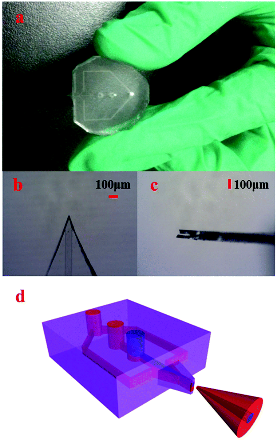 | ||
| Fig. 1 (a) Photograph of the 3D HFNE, (b) the ESI emitter of the 3D HFNE under a microscope, (c) the side view of the emitter tip under a microscope, and (d) the simulation of the wrapped charged aerosol plume from the 3D HFNE. | ||
In the fabrication of the 3D HFNE, the second and the third layer on the molds were baked at 90 °C for 18 min, and immediately pasted with the first and the fourth layer, respectively. Both combinations, which were baked at 90 °C for 2 h, were peeled off and successively immersed in acetone and methanol for 2 h to remove possible oligomers of PDMS. After that, they were cleaned, punched and treated in plasma for the final fabrication. Then, the prepared device was baked at 120 °C for 48 h to pursue a complete polymerization, and was cut along reference lines reserved in the second layer under a microscope (Jiangnan, China) to prepare the emitter tip.
Three-dimensional hydrodynamic focusing in 3D HFNE
The sample flow and two focusing flows were injected into the corresponding inlets as indicated in Fig. S2.† Because of the laminar flow feature in microfluidics, the sample flow in the 3D HFNE would be condensed by horizontal and vertical focus flows as indicated in Fig. 1(d). In this case, the sample flow would be wrapped in the whole charged aerosol plume. In order to verify this hypothesis, Coomassie blue (CB) and RhB, as the sample solution and two focus solutions, were employed to develop the wrapped electrospray. Because of the obvious ion expansion phenomenon during the ESI process, approximately symmetrical patterns were observed, and the distribution of the sample flow in the aerosol charged plume may be distributed in the central region as illustrated in Fig. 1(d). As shown in Fig. S3,† deposition patterns from the proposed 3D HFNE were collected on filter papers, which were pasted on conductive aluminium foil.3D HFNE coupled with TOF-MS
The instrumental configuration to couple the 3D HFNE with TOF-MS is illustrated in Fig. 2. Syringe pumps (Longer Pump, China) were employed to infuse solutions and control their flow rates. Tubing (0.8 mm i.d. and 1.6 mm o.d.) was inserted into the corresponding inlets to introduce various solutions. A high-voltage power supply (Dongwen, China) was connected with a platinum electrode, which was inserted into a T-shaped adaptor to apply a voltage to the horizontal focus flow. As shown in Fig. 2, the proposed 3D HFNE was positioned on an xyz regulator, which was used to align the distribution of sample ions (in blue colour) toward the ion transmission orifice, which had a 600 μm diameter. Prior to MS determinations, the position of the 3D HFNE was fully optimized by obtaining the strongest sample ion intensity for a standard chemical, e.g., reserpine. A 6224 TOF mass spectrometer (Agilent, USA) was coupled with the 3D HFNE, and a manual injection valve (Agilent, USA) was employed to achieve the sample injection. A practical photograph of the on-line combination of 3D HFNE and TOF-MS is shown in Fig. S4.†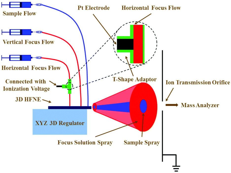 | ||
| Fig. 2 The instrumental configuration of 3D HFNE coupled with TOF-MS. | ||
Chemicals
A conductive mixture (CH3OH![[thin space (1/6-em)]](https://www.rsc.org/images/entities/char_2009.gif) :H2O:CH3COOH = 80:19.9:0.1, v/v/v) was used as the horizontal and vertical focus flows in all experiments. PDMS (GE, USA) was employed to fabricate the proposed emitter. CB, RhB, metamifop, isoprothiolane and reserpine were purchased from Sigma-Aldrich (St. Louis, USA), and all solvents were from Merck (Darmstadt, Germany). The double distilled water used in this work was from a water purifier system (Millipore, USA), and its conductivity was 18.2 MΩ cm.
:H2O:CH3COOH = 80:19.9:0.1, v/v/v) was used as the horizontal and vertical focus flows in all experiments. PDMS (GE, USA) was employed to fabricate the proposed emitter. CB, RhB, metamifop, isoprothiolane and reserpine were purchased from Sigma-Aldrich (St. Louis, USA), and all solvents were from Merck (Darmstadt, Germany). The double distilled water used in this work was from a water purifier system (Millipore, USA), and its conductivity was 18.2 MΩ cm.
Results and discussion
Confirmation of the wrapped nanoelectrospray
In order to confirm our hypothesis, various deposition patterns from the 3D HFNE were collected and compared under different infusion conditions as shown in Fig. 3. Firstly, homogenous red patterns were obtained when RhB solution was employed as the sample flow and two focus flows. Moreover, the patterns in Fig. 3 were obtained when blue coloured CB was used as the sample flow. There were obvious blue and red regions in all patterns. This was different from the preceding homogenous patterns, and this phenomenon preliminarily supported the proposed wrapped electrospray.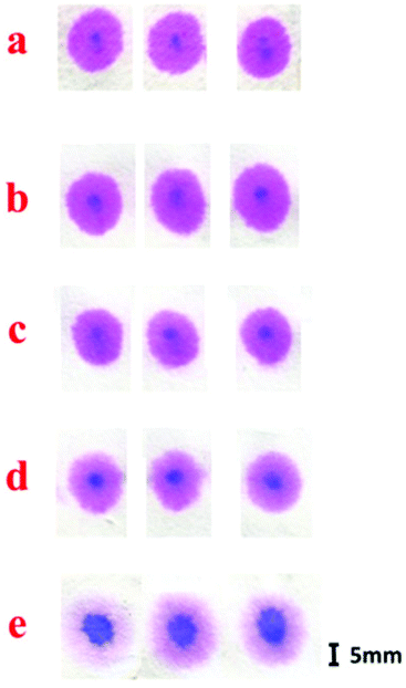 | ||
| Fig. 3 Deposition patterns of the wrapped charged aerosol plume under different sample flow rates and focus flow rates for 15 min. The distance between the paper and the 3D HFNE was around 6 mm, which was revealed to be an optimized parameter in the proposed method. Coomassie blue solution (8 ng μL−1) in blue and RhB solution (8 ng μL−1) in red were employed as the sample flow and two focusing flows, respectively. Infusion rates of the sample flow and two focusing flows (horizontal and vertical directions) were set as: (a) 0.15 μL min−1, 2 μL min−1 and 1.5 μL min−1; (b) 0.15 μL min−1, 2 μL min−1 and 1 μL min−1; (c) 0.15 μL min−1, 1 μL min−1 and 1 μL min−1; (d) 0.5 μL min−1, 1 μL min−1 and 1 μL min−1 and (e) 1.5 μL min−1, 1 μL min−1 and 1 μL min−1. | ||
In addition, the blue region, corresponding to the sample distribution, significantly shrank with the reduction of the infusion rate of the sample flow as shown in Fig. 3(c–e). This indicated the feasibility of restraining the sample expansion in the wrapped nanoelectrospray. In this way, the actual distribution of the sample ions could be regulated to be matched with the ion transmission orifice (600 μm i.d.) in the mass spectrometer, and the injection loss could, to an extent, be inhibited. Furthermore, the blue regions in Fig. 3(a–c) became smaller with greater infusion rate ratios between the two focus flows and the sample flow. This further supported the effect of the proposed 3D HFNE on confining the sample ion expansion. Finally, blue regions were clearly observed when the sample flow was infused at 0.15 μL min−1. This may stand for a decent signal-to-noise ratio (s/n) at this infusion rate. Overall, all deposition patterns supported the configuration of the proposed wrapped electrospray.
It is worth pointing out that the blue regions slightly deviated upward from the centre in all patterns. This would probably be because the sample flow was directly focused by the vertical focusing flow from its bottom as shown in Fig. 1(d). This phenomenon could be eliminated by applying two focusing flows from the top and the bottom of the sample flow, respectively. However, it failed to improve either the sensitivity of the 3D HFNE or its lowest infusion rate, and made the configuration of the proposed emitter as well as its applications more complicated. Therefore, the 3D HFNE was proposed as in Fig. 1.
In addition, the distribution of the sample ions was further evaluated to confirm the proposed wrapped electrospray. The ion intensities of the sample, metamifop, were compared at different lateral and vertical displacements. They indicated that the distribution of the sample in the wrapped spray was obviously more focused in the central region, and its achieved maximum ion intensities were improved in the wrapped spray. Moreover, the ion intensity ratios between metamifop and isoprothiolane, which stood for the sample and focusing flows, were collected. Despite identical amounts of metamifop and isoprothiolane being applied in wrapped and homogeneous sprays, the best ratios in both directions were always obtained in the wrapped one.
The ratios between metamifop (providing the analyte ion) and isoprothiolane (providing the background ion) were collected at different radial distances, and a ∼6 mm distance from the ion transmission orifice provided the best inhibition of sample expansion as indicated in Fig. S5.† When the distance was less than the preceding optimal value, the sample ions would not expand to a size which could cover the ion transmission orifice as much as possible, and this would lower the sensitivity due to more transmitted background ions. On the contrary, the sample ions would expand to a greater distribution than the ion transmission orifice when the distance was larger than the preceding optimal value, and more background ions from isoprothiolane would expand into the central region. This process was in fact equal to a dilution for the sample ion, which would result in comparably worse detection.
Performance evaluation for 3D HFNE
Metamifop was employed to evaluate the sensitivity of the 3D HFNE, which was compared with a reported nanoESI emitter. The molecular ions of metamifop and isoprothiolane were obtained using the 3D HFNE as shown in Fig. 4(a and b) with infusion rates of 0.3 μL min−1 and 0.15 μL min−1, respectively. In order to compare the effect of three-dimensional hydrodynamic focusing in the proposed device, it was compared with a reported nanoESI emitter with fully optimized positions and parameters.23 It could be observed that the proposed 3D HFNE provided a better performance compared with the reported emitter when 150 pg of metamifop was determined (Fig. S6(a and b)†), and its limit of detection (s/n = 3) was evaluated to be 30 pg, which was an approximately 11.3% improvement. Moreover, RhB was determined to evaluate the sensitivity of the 3D HFNE compared with a commercial ESI source, which has already been optimized to the best conditions by the producer, to evaluate the advantage of inhibiting ion expansion with the proposed device. As shown in Fig. 4(c), the quasi-molecular ion of RhB was obtained based on the proposed emitter at m/z 443 at a 0.15 μL min−1 infusion rate. The achieved limit of detection (s/n = 3) based on the 3D HFNE was around 1 pg for RhB, and this value was better than its counterpart using the commercial ESI source (Fig. S6(c and d)†).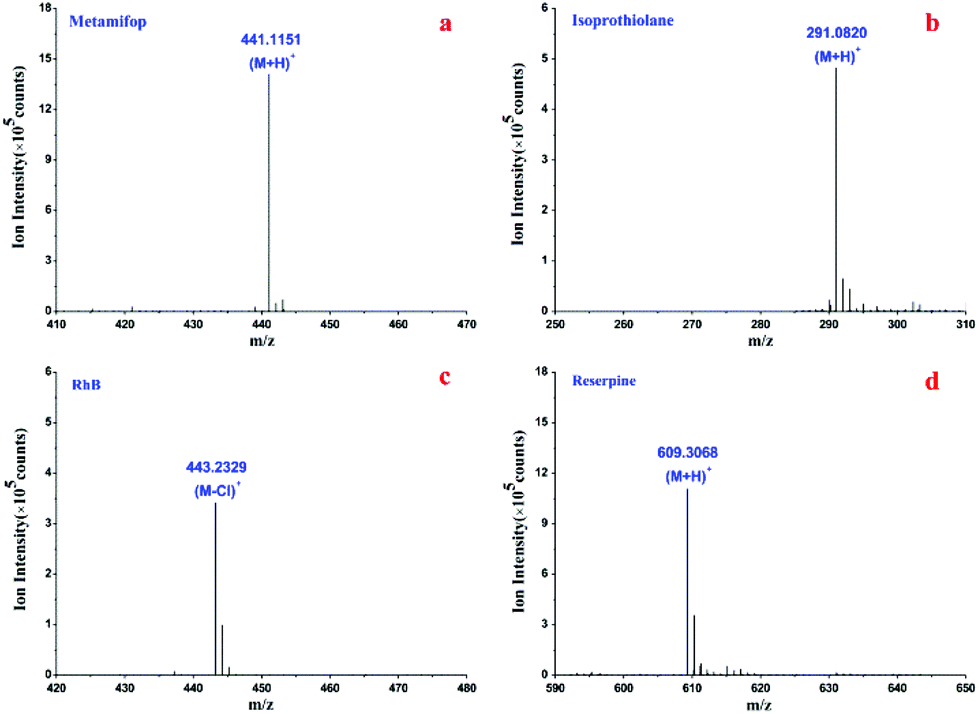 | ||
| Fig. 4 MS spectra of metamifop, isoprothiolane, RhB and reserpine based on the 3D HFNE. Infusion rates of the sample flow, and the horizontal and the vertical focusing flows were (a) metamitop (5 ng μL−1), 0.3 μL min−1, 1.2 μL min−1, 0.2 μL min−1; (b) isoprothiolane (5 ng μL−1), 0.15 μL min−1, 1 μL min−1, 0.2 μL min−1; (c) RhB (2 ng μL−1), 0.15 μL min−1, 3 μL min−1 and 0.8 μL min−1; and (d) reserpine (5 ng μL−1), 800 nL min−1, 3 μL min−1, 800 nL min−1. | ||
Reserpine was utilized to evaluate the performance of the 3D HFNE. With an 800 nL min−1 infusion rate, its achieved s/n was over 5 as shown in Fig. 4(d), and the relative standard deviation (RSD) of the total ion chromatograms (TIC) for reserpine in Fig. 4(d) was 3.61% within 6 min (Fig. S7†). Reserpine was also determined under different voltages and infusion rate ratios between the sample flow and two focusing flows. As shown in Table 1, the RSDs in the first and last three rows became worse with decreasing infusion rate ratios, and the stability of the proposed method improved when the voltage decreased from 4500 V to 3500 V. Moreover, the RSDs became worse with decreasing sample flow rates from the third row to the sixth row, in which all flow rate ratios remained constant. This would probably be due to lower sample flow rates, which would be accompanied by comparably greater errors in their infusion control. Generally, a reliable ionization for reserpine has been obtained based on the proposed 3D HFNE when the sample flow rate was no less than 0.03 μL min−1.
| Voltage (V) | Infusion rates (μL min−1) | RSD (n = 10, %) | ||
|---|---|---|---|---|
| Horizontal focusing | Vertical focusing | Sample flow | ||
| 3500 | 3 | 0.8 | 0.8 | 3.61 |
| 3500 | 3 | 0.8 | 0.5 | 4.56 |
| 3500 | 3 | 0.8 | 0.3 | 6.25 |
| 3500 | 0.5 | 0.13 | 0.05 | 7.43 |
| 3500 | 0.3 | 0.08 | 0.03 | 8.94 |
| 3500 | 0.1 | 0.03 | 0.01 | 11.5 |
| 4500 | 3 | 0.8 | 0.8 | 7.67 |
| 4500 | 3 | 0.8 | 0.5 | 7.97 |
| 4500 | 3 | 0.8 | 0.3 | 10.2 |
Based on the optimal proposed method, the achieved MS spectra of reserpine at 150 nL min−1 and 30 nL min−1 were compared. Firstly, the molecular ion of reserpine (m/z 609) was observed with a 150 nL min−1 flow rate, and its s/n for 5 μg mL−1 reserpine was over 4 (Fig. S8(a)†). Furthermore, the molecular ion of reserpine was obtained with a 30 nL min−1 infusion rate, while its s/n was less than 3 (Fig. S8(b)†). The ion intensities of reserpine increased from 6.8 × 10⁴ to 1.2 × 10⁵, when its flow rate changed from 30 nL min−1 to 150 nL min−1. The decreased ion intensity, which corresponded to a lower infusion rate, further indicated the reliability of the proposed 3D HFNE.
Compatibility and durability of 3D HFNE
The proposed 3D HFNE was employed to determine RhB dissolved in various compositions of methanol and water, including 100% methanol and 100% water. It was compatible with all dissolved solutions, and stable sprays were achieved with any composition. This was probably because the two focus flows, which contained 80% methanol, 19.9% water and 0.1% formic acid, had a greater infusion rate compared with the sample. Their high proportion actually stabilized the composition of the whole flow, and ensured its volatility and conductivity, both of which were indispensable in the electrospray.The durability of the 3D HFNE was also evaluated using its determinations for 5 μg mL−1 reserpine at a 0.3 μL min−1 flow rate, and one 3D HFNE was evaluated 1 d, 7 d, 30 d and 90 d after its preparation. In all determinations, stable sprays were always formed, while the RSD at 90 d was 15.3%, which was worse than the performance at 1 d (6.25%), 7 d (6.98%) and 30 d (9.17%). This may be due to the aging of PDMS in the air as well as its extraction of various gaseous chemicals, which would be intermittently ionized by the 3D HFNE.
The compatible infusion rate range of the proposed 3D HFNE was evaluated to be from 0.01 μL min−1 to 15 μL min−1 by infusing isoprothiolane solution. Within the preceding range, stable nanoelectrosprays were always observed. When the sample flow rate was over 15 μL min−1, the proposed emitter would frequently crack due to the high hydraulic pressure.
Conclusions
We have developed a new 3D HFNE method to achieve a wrapped nanoelectrospray based on three-dimensional hydrodynamic focusing. Electrospray deposition patterns and the comparison of the sample ion distribution between a wrapped spray and a homogeneous spray confirmed its capacity to regulate the sample ion distribution in the wrapped electrospray. In this way, ion expansion during sample injection was inhibited. After full optimization of the ionization voltage, the radial distance and various infusion rates, the proposed 3D HFNE achieved an improved sensitivity compared with a reported nanoESI emitter and a commercial source. It was indicated to be compatible with a wide infusion rate range, from 0.01 μL min−1 to 15 μL min−1, and various solution compositions, including 100% methanol and 100% water. Its durability and stability were evaluated to be acceptable. The imperfect limit of detection relates to the dissolution of PDMS monomers, which results in ionization suppression and lowers the sensitivity. If an effective strategy could be employed to restrain the dissolution of PDMS monomers, an improved sensitivity may be obtained. Considering its low cost and user-friendly properties, the 3D HFNE would be a potential option to achieve nanoESI-MS determinations using microfluidics with conventional mass spectrometers.Acknowledgements
We sincerely acknowledge Prof. Hongying Zhong in CCNU for helpful discussions. This research was financially supported by self-determined research funds of CCNU from the colleges’ basic research and operation of MOE (CCNU14A05005, and CCNU15KFY004), and the National Natural Science Foundation of China (21205044).Notes and references
- C. A. Smith, X. Li, T. H. Mize, T. D. Sharpe, E. I. Graziani, C. Abell and W. T. S. Huck, Anal. Chem., 2013, 85, 3812–3816 CrossRef CAS PubMed.
- A. Arora, G. Simone, G. B. Salieb-Beugelaar, J. T. Kim and A. Manz, Anal. Chem., 2010, 82, 4830–4847 CrossRef CAS PubMed.
- T.-C. Chao and N. Hansmeier, Proteomics, 2013, 13, 467–479 CrossRef CAS PubMed.
- J. Avesar, T. Ben Arye and S. Levenberg, Lab Chip, 2014, 14, 2161–2167 RSC.
- T. Haselgruebler, M. Haider, B. Ji, K. Juhasz, A. Sonnleitner, Z. Balogi and J. Hesse, Anal. Bioanal. Chem., 2014, 406, 3279–3296 CrossRef CAS PubMed.
- N.-T. Huang, H.-l. Zhang, M.-T. Chung, J. H. Seo and K. Kurabayashi, Lab Chip, 2014, 14, 1230–1245 RSC.
- Z. Wei, S. Han, X. Gong, Y. Zhao, C. Yang, S. Zhang and X. Zhang, Angew. Chem., Int. Ed., 2013, 52, 11025–11028 CrossRef CAS PubMed.
- N. Gasilova, L. Qiao, D. Momotenko, M. R. Pourhaghighi and H. H. Girault, Anal. Chem., 2013, 85, 6254–6263 CrossRef CAS PubMed.
- A. E. Kirby, N. M. Lafreniere, B. Seale, P. I. Hendricks, R. G. Cooks and A. R. Wheeler, Anal. Chem., 2014, 86, 6121–6129 CrossRef CAS PubMed.
- X. Wang, L. Yi, N. Mukhitov, A. M. Schrell, R. Dhumpa and M. G. Roper, J. Chromatogr., A, 2015, 1382, 98–116 CrossRef CAS PubMed.
- X. He, Q. Chen, Y. Zhang and J.-M. Lin, Trends Anal. Chem., 2014, 53, 84–97 CrossRef CAS.
- Q. Chen, J. Wu, Y. Zhang and J.-M. Lin, Anal. Chem., 2012, 84, 1695–1701 CrossRef CAS PubMed.
- D. Gao, H. Liu, Y. Jiang and J.-M. Lin, Lab Chip, 2013, 13, 3309–3322 RSC.
- R. T. Kelly, J. S. Page, Q. Luo, R. J. Moore, D. J. Orton, K. Tang and R. D. Smith, Anal. Chem., 2006, 78, 7796–7801 CrossRef CAS PubMed.
- X. Li, D. Xiao, X.-M. Ou, C. McCullm and Y.-M. Liu, J. Chromatogr., A, 2013, 1318, 251–256 CrossRef CAS PubMed.
- A. G. Chambers and J. M. Ramsey, Anal. Chem., 2012, 84, 1446–1451 CrossRef CAS PubMed.
- P. Hoffmann, M. Eschner, S. Fritzsche and D. Belder, Anal. Chem., 2009, 81, 7256–7261 CrossRef CAS PubMed.
- W. Kim, M. Guo, P. Yang and D. Wang, Anal. Chem., 2007, 79, 3703–3707 CrossRef CAS PubMed.
- L. Sainiemi, T. Sikanen and R. Kostiainen, Anal. Chem., 2012, 84, 8973–8979 CAS.
- S. Arscott, Lab Chip, 2014, 14, 3668–3689 RSC.
- Y. Lu, F. Liu, N. Lion and H. H. Girault, J. Am. Soc. Mass Spectrom., 2013, 24, 454–457 CrossRef CAS PubMed.
- R. T. Kelly, K. Q. Tang, D. Irimia, M. Toner and R. D. Smith, Anal. Chem., 2008, 80, 3824–3831 CrossRef CAS PubMed.
- X. F. Sun, R. T. Kelly, K. Q. Tang and R. D. Smith, Anal. Chem., 2011, 83, 5797–5803 CrossRef CAS PubMed.
- X. Sun, R. T. Kelly, K. Tang and R. D. Smith, Analyst, 2010, 135, 2296–2302 RSC.
- R. T. Kelly, J. S. Page, Q. Z. Luo, R. J. Moore, D. J. Orton, K. Q. Tang and R. D. Smith, Anal. Chem., 2006, 78, 7796–7801 CrossRef CAS PubMed.
- N. G. Batz, J. S. Mellors, J. P. Alarie and J. M. Ramsey, Anal. Chem., 2014, 86, 3493–3500 CrossRef CAS PubMed.
- T. C. Rohner, J. S. Rossier and H. H. Girault, Anal. Chem., 2001, 73, 5353–5357 CrossRef CAS PubMed.
- D. S. Liu, B. Hakimi, M. Volny, J. Rolfs, X. D. Chen, F. Turecek and D. T. Chiu, Anal. Chem., 2013, 85, 6190–6194 CrossRef CAS PubMed.
- P. Mao, R. Gomez-Sjoberg and D. Wang, Anal. Chem., 2013, 85, 816–819 CrossRef CAS PubMed.
- B. R. Reschke and A. T. Timperman, J. Am. Soc. Mass Spectrom., 2011, 22, 2115–2124 CrossRef CAS PubMed.
- L. F. Cai, Y. Zhu, G. S. Du and Q. Fang, Anal. Chem., 2012, 84, 446–452 CrossRef CAS PubMed.
- Y. Zhu and Q. Fang, Anal. Chem., 2010, 82, 8361–8366 CrossRef CAS PubMed.
- P. Kebarle and L. Tang, Anal. Chem., 1993, 65, 972A–986A CAS.
- I. Marginean, R. T. Kelly, D. C. Prior, B. L. LaMarche, K. Tang and R. D. Smith, Anal. Chem., 2008, 80, 6573–6579 CrossRef CAS PubMed.
- S. F. W. Bakhoum and G. R. Agnes, Anal. Chem., 2005, 77, 3189–3197 CrossRef CAS PubMed.
- S. F. W. Bakhoum, M. J. Bogan and G. R. Agnes, Anal. Chem., 2005, 77, 3461–3465 CrossRef CAS PubMed.
- G. T. T. Gibson, R. D. Wright and R. D. Oleschuk, J. Mass Spectrom., 2012, 47, 271–276 CrossRef CAS PubMed.
- R. T. Kelly, J. S. Page, I. Marginean, K. Tang and R. D. Smith, Anal. Chem., 2008, 80, 5660–5665 CrossRef CAS PubMed.
- C. H. Xie, M. L. Ye, X. G. Jiang, W. H. Jin and H. F. Zou, Mol. Cell. Proteomics, 2006, 5, 454–461 CAS.
- G. Hairer, G. S. Paerr, P. Svasek, A. Jachimowicz and M. J. Vellekoop, Sens. Actuators, B, 2008, 132, 518–524 CrossRef CAS.
- M. G. Lee, S. Choi and J.-K. Park, Lab Chip, 2009, 9, 3155–3160 RSC.
- M. Lu, Y.-P. Ho, C. L. Grigsby, A. A. Nawaz, K. W. Leong and T. J. Huang, ACS Nano, 2014, 8, 332–339 CrossRef CAS PubMed.
- M. Lu, S. Yang, Y.-P. Ho, C. L. Grigsby, K. W. Leong and T. J. Huang, ACS Nano, 2014, 8, 10026–10034 CrossRef CAS PubMed.
- M. A. Daniele, D. A. Boyd, D. R. Mott and F. S. Ligler, Biosens. Bioelectron., 2015, 67, 25–34 CrossRef CAS PubMed.
Footnote |
| † Electronic supplementary information (ESI) available: Additional figures. See DOI: 10.1039/c5an01619c |
| This journal is © The Royal Society of Chemistry 2016 |