
 Open Access Article
 This Open Access Article is licensed under a
 Creative Commons Attribution 3.0 Unported Licence
Trains, tails and loops of partially adsorbed semi-flexible filaments†‡
David
Welch
a,
M. P.
Lettinga
bc,
Marisol
Ripoll
d,
Zvonimir
Dogic
*e and
Gerard A.
Vliegenthart
*f
aGraduate Program in Biophysics and Structural Biology, Brandeis University, Waltham, MA 02454, USA
bSoft Matter, Institute of Complex Systems, Forschungszentrum Jülich, D-52425 Jülich, Germany
cKU Leuven, Laboratory for Soft Matter and Biophysics, Celestijnenlaan 200D, B-3001 Leuven, Belgium
dTheoretical Soft Matter and Biophysics, Institute of Complex Systems, Forschungszentrum Jülich, D-52425 Jülich, Germany
eDepartment of Physics, Brandeis University, Waltham, MA 02454, USA. E-mail: zdogic@brandeis.edu
fTheoretical Soft Matter and Biophysics, Institute for Advanced Simulation, Forschungszentrum Jülich, D-52425 Jülich, Germany. E-mail: g.vliegenthart@fz-juelich.de
First published on 7th August 2015
Abstract
Polymer adsorption is a fundamental problem in statistical mechanics that has direct relevance to diverse disciplines ranging from biological lubrication to stability of colloidal suspensions. We combine experiments with computer simulations to investigate depletion induced adsorption of semi-flexible polymers onto a hard-wall. Three dimensional filament configurations of partially adsorbed F-actin polymers are visualized with total internal reflection fluorescence microscopy. This information is used to determine the location of the adsorption/desorption transition and extract the statistics of trains, tails and loops of partially adsorbed filament configurations. In contrast to long flexible filaments which primarily desorb by the formation of loops, the desorption of stiff, finite-sized filaments is largely driven by fluctuating filament tails. Simulations quantitatively reproduce our experimental data and allow us to extract universal laws that explain scaling of the adsorption–desorption transition with relevant microscopic parameters. Our results demonstrate how the adhesion strength, filament stiffness, length, as well as the configurational space accessible to the desorbed filament can be used to design the characteristics of filament adsorption and thus engineer properties of composite biopolymeric materials.
I. Introduction
In comparison to simple rigid molecules whose adsorption can be described by straightforward two-state models, the adsorption of complex molecules with internal degrees of freedom, such as polymeric chains, requires development of more intricate theories. The complication arises because certain segments of an adsorbed filament can be surface bound while other segments within the same molecule remain desorbed. This qualitative change in behavior requires development of theoretical models of adsorption transition that can account for internal degrees of freedom of polymeric chains.1–12 At a fundamental level the configurations of a partially adsorbed polymer can be described in terms of trains, tails and loops.12–15 Trains are polymer segments that are adsorbed onto a surface, loops are desorbed segments separated by two trains while tails account for the desorbed end segments. Traditional scattering-based experimental techniques used to investigate polymer adsorption do not directly reveal the statistics of tails, trains and loops.16,17 Instead they yield structural information that is averaged over many states and molecules and as as such it cannot be used to directly extract conformational statistics of partially adsorbed filaments.Microscopy has significantly advanced polymer science by enabling single-molecule visualization of structures and dynamical processes that could previously be only studied by bulk techniques. It has been used to visualize dynamics of desorbed 3D polymers as well as filaments that are strongly adsorbed onto the substrate so that they effectively behave as a 2D system.19–23 Here we bridge these two previously studied limits by visualizing 3D configurations of semi-flexible filaments as they undergo an adsorption/desorption transition. We examine how the strength of the polymer-wall attractions affects the statistics of trains, tails and loops. This information is used to estimate the location of the adsorption–desorption transition. We study the same processes using computer simulations and find quantitative agreement with the experimental measurements. In contrast to desorption of flexible chains which is dominated by loop formation, the desorption of finite length semi-flexible filaments is largely driven by tail fluctuations. With decreasing attraction strength the average tail length increases up to the point where it is comparable to the filament contour length, whereupon the entire filament desorbs from the surface. The statistics of filament loops, tails and trains and their dependence on attraction strength is in broad agreement with computer simulation that have previously studied similar phenomena.24,25
II. Experimental methods
For experimental work we used phalloidin stabilized F-actin filaments, which have 6 nm diameter and a persistence length of 16 μm.26 The large persistence length allowed us to reconstruct the entire 3D filament conformation. Negatively charged F-actin filaments are repelled from a glass surface of the same charge. To induce a tunable filament-wall attraction we added non-adsorbing polymer dextran (MW 500![[thin space (1/6-em)]](https://www.rsc.org/images/entities/char_2009.gif) 000, Sigma), which has a radius of gyration Rg ∼ 18 nm.27 The dextran center of mass is excluded from a layer of thickness Rg adjacent to a hard wall as well as from a shell of radius Rg + Rf, where Rf = 3 nm is the radius of the filament, surrounding each filament. As F-actin approaches the wall, the two excluded volume regions overlap, leading to increase in the total volume accessible to the depleting polymers and attractive wall-filament depletion interactions.28,29 All experiments were performed in the dilute regime, ensuring that the actin–substrate interaction strength is linearly proportional to the dextran concentration. The instantaneous 3D configurations of a partially adsorbed filament were extracted from Total Internal Reflection Fluorescence (TIRF) Microscopy images. In the evanescent field the excitation intensity decays exponentially; consequently, the filament distance away from the wall is directly related to its local intensity.30 Combining depletion interaction with TIRF imaging allowed us to tune the strength of filament-wall attractive potential while simultaneously visualizing the entire 3D filaments configuration with nanometer accuracy (Fig. 1a and b).
000, Sigma), which has a radius of gyration Rg ∼ 18 nm.27 The dextran center of mass is excluded from a layer of thickness Rg adjacent to a hard wall as well as from a shell of radius Rg + Rf, where Rf = 3 nm is the radius of the filament, surrounding each filament. As F-actin approaches the wall, the two excluded volume regions overlap, leading to increase in the total volume accessible to the depleting polymers and attractive wall-filament depletion interactions.28,29 All experiments were performed in the dilute regime, ensuring that the actin–substrate interaction strength is linearly proportional to the dextran concentration. The instantaneous 3D configurations of a partially adsorbed filament were extracted from Total Internal Reflection Fluorescence (TIRF) Microscopy images. In the evanescent field the excitation intensity decays exponentially; consequently, the filament distance away from the wall is directly related to its local intensity.30 Combining depletion interaction with TIRF imaging allowed us to tune the strength of filament-wall attractive potential while simultaneously visualizing the entire 3D filaments configuration with nanometer accuracy (Fig. 1a and b).
 | ||
| Fig. 1 TIRF microscopy determines 3D conformations of a fluctuating filament undergoing adsorption/desorption transition. (a) Schematic of the experimental setup. An evanescent field is achieved by refracting laser through a prism above the critical angle θc. The sample is viewed from below with a high numerical aperture (NA) objective. A polymer brush coating the coverslip surface ensures that filaments adsorb only to the top surface. (b) The filament height plotted as a function of its position makes it possible to identify tails, trains and loops. The local height, h, is extracted from the filament intensity according to the relationship, h = −aln(I/I0) where I is the intensity at a given height, I0 the contour's maximum intensity (an offset is subtracted from both) and a is a decay constant of the evanescent field. Inset: Image of the filaments from which the height information is extracted. (c) TIRF (top) and corresponding epi-fluorescence (bottom) images of adsorbed filaments at three different dextran concentrations corresponding to (i) the desorbed regime, (ii) the transition region and (iii) strongly adsorbed regime. For related movies see ref. 36. (d) Snapshots of filament configuration obtained with computer simulations corresponding to three regime. | ||
For reproducible results we used cover slides from the same production batch (VWR). The slides where incubated in 6 M HCl for 45 minutes, rinsed with deionized water and sonicated in hot soap water (1% Hellmanex, Hellma) for five minutes before final rinsing and storage in ddH2O. Slides were used within 24 hours of cleaning. To adsorb filaments only on one surface, the coverslip surface was coated with a poly-acrylamide brush which suppresses wall-filament depletion interactions.31,32 Actin was column-purified, polymerized and labelled with Alexa-488 phalloidin, at 1:1 monomer:dye ratio.33 F-actin filaments were dissolved in buffer containing 20 mM NaH2PO4 (pH = 7.4), 200 mM KCl, and 30% sucrose (w/v). Sucrose slows down desorption of Alexa-488 phalloidin and thus prolongs the observation time of F-actin filaments.34 Actin filaments are inherently polydisperse; for our analysis we only used filaments that are larger than the persistence length. The average length of the analyzed filaments was 33 μm which is roughly twice the persistence length. For each dextran concentration we have analyzed on average five different filaments of comparable contour length.
We used a prism-based TIRF setup since it produces evanescent fields with low background fluorescence and a better defined exponential decay length.30 Phalloidin labelled actin filaments exhibit a pronounced polarization dependent fluorescence signal.35 In order to minimize this contribution we ensured that the polarization of the laser was in the plane defined by the incident and reflected light.30 To determine the accuracy of our method we have imaged filaments that are irreversibly attached to the surface and thus exhibited no height fluctuations. Intensity fluctuation of such filaments corresponded to apparent height variations of ±40 nm; hence we estimate that our resolution is about 80 nm. The fluorescence images were acquired using an EMCCD operating in a conventional mode (Andor iXon), mounted on a Nikon ecclipseTE-2000 microscope and using a PlanFluor-100× NA 1.3 objective. The time between exposures was 2 seconds ensuring that the subsequent images were uncorrelated. We imaged a single filament for approximately 200 frames before photobleaching effects began to influence chain statistics. In parallel with TIRF imaging, filaments were simultaneously visualized with epi-fluorescence microscopy which enabled determination of the filament contour length. To experimentally measure the evanescent field decay constant we prepared chambers of well-defined thickness that ranged between 1 and 2 μm with 100 nm beads adsorbed onto both surfaces. The chamber thickness was accurately measured by an objective mounted on a piezo-stage. Knowing the chamber thickness and measuring the ratio of bead intensities attached to opposite surface directly yields the decay constant of the evanescent field. The TIRF decay length measured in this way was Ξ = 230 ± 40 nm. This is close to theoretical predictions  , where θc is the critical angle, θ = 61° is the incident angle away from the normal to the imaging plane and λ = 488 nm the wavelength of the beam. Using samples with homogeneous fluorescence we calibrated for the non-uniform intensity of the TIRF excitation field in the image plane. In order to analyze the data, we classified all filament segments closer than 80 nm to the cover slide as adsorbed. To investigate the influence of chamber thickness, we have studied the adsorption/desorption of actin filaments in chambers with thickness 2 and 10 μm. Such chambers were prepared by using 2 and 10 μm beads as spacers.
III. Simulations
The adsorption experiments have been complemented by off-lattice Monte Carlo computer simulations of a single non-grafted polymer filament of length L and persistence length Lp, confined between two flat walls separated by a distance Lz. For not too long polymers (L/Lp ≈ 1), in which self-avoidance effects are negligible, a description in the worm-like chain model is appropriate.37,38 Each semi-flexible polymer was described by N inextensible infinitely thin elements of length l0 = L/N and a bending potential Vb = κ(1 − ti·ti+1)/l0 between subsequent segments. Here ti is the unit tangent vector at the i-th segment in the chain, and κ the bending stiffness. The persistence length Lp is defined by 〈ti·tj〉/d = exp[−(d − 1)sij/Lp] for unconfined filaments, where sij is the distance between two segments along the contour and d the embedding dimensionality. The persistence length is related to the bending rigidity by Lp = 2κ/kBT with kBT the thermal energy.39,40 The filament interaction with the walls is included as a hard-core repulsive interaction. Similar to the experimental system, one of the walls (in fact the lower one) is made attractive by superimposing an attractive square well interaction of range δ and depth ε =![[small epsilon, Greek, tilde]](https://www.rsc.org/images/entities/i_char_e0de.gif) /kBT on top of the repulsive interaction. Here is the bare interaction strength per unit length of polymer. The interaction strength was varied by changing and keeping the temperature (and thus the persistence length) constant. This is similar to depletion induced attractions where the strength of the attraction is tuned by the concentration of depletant and not by variation of temperature.
/kBT on top of the repulsive interaction. Here is the bare interaction strength per unit length of polymer. The interaction strength was varied by changing and keeping the temperature (and thus the persistence length) constant. This is similar to depletion induced attractions where the strength of the attraction is tuned by the concentration of depletant and not by variation of temperature.
The Monte Carlo simulations involved pivot configurational moves in two and three dimensions,41,42 uniform translations perpendicular to the wall and uniform rotational moves. Parameters in the simulations were chosen to resemble those in the experiments, and results are discussed in terms of dimensionless quantities. We used filaments of Lp = 16, and L = 33, such that L/Lp ≃ 2.1. For a large enough number of segments N (l0 small enough) the results are independent of the discretization. N was estimated from the transversal deviation 〈b2(s)〉 = 2s3/3Lp of a semi-flexible polymer from its initial direction.43 By identification of s with the segment length L/N, b with the range of the attraction and arguing that the transversal crossing of the attraction well should require more than one step we find that s < (3Lpδ2/2)1/3. Averages were calculated over adsorbed configurations which have non-zero filament fraction within a cut-off distance Rc from the wall. The parameters chosen for the attractive wall are δ = 0.01 such that δ/L ≃ 0.0004 and Rc = 8δ. Our work examined the effect of confinement on adsorption transition of filament with both free ends, in contrast to other simulations that examined transitions of unconfined filaments which were grafted at one end.18,24 We calculate the average length of tails, trains and loops and normalize them by the filament persistence length Lp, since it is uniquely defined in both simulations and experiments. This in contrast to the polymer contour length L which is subject to the intrinsic polydispersity of experimental samples.
IV. Results & discussion
At low depletant concentrations (weak adsorption limit) the vast majority of filaments are largely desorbed from the wall (Fig. 1b and c(i)). When such samples are viewed with TIRF microscopy, one occasionally observes short filament segments that briefly remain in the evanescent field. Increasing the depletant concentration leads to a transition regime where the length of the adsorbed segments increases (Fig. 1b and c(ii)). Here, filaments remain attached to the surface on timescales longer than the duration of the experiment while exhibit large fluctuations. At even higher depletant concentrations (strong adsorption limit) almost entire filament is permanently adsorbed on the interface. One can occasionally identify desorbed short segments that are either located in the middle of the filament or at its ends. (Fig. 1b and c(iii), for related movies see ref. 36). Qualitatively similar filament behavior is observed in computer simulations, Fig. 1d shows typical snapshots for adsorption strengths where the filament is weakly bound (i), where a loop is present (ii) and for strong attractions where the filament is tightly bound to the surface and exhibits only one train (iii).To quantify these observations we have measured how the average length of filament trains, tails and loops depend on the strength of the filament-wall attraction. For strongest attractions, fluctuations away from the surface are almost completely suppressed and the average train length 〈Ltrain〉 approaches the filament contour length, L (Fig. 2a). In this limit the average length of tails and loops is negligible. With decreasing attraction strength the filament starts to fluctuate away from the minimum energy state by locally desorbing from a flat surface, at first slightly but in the transition regime 〈Ltrain〉 drops precipitously, approaching almost zero for very weak attractions (desorbed filaments). The transition regime is clearly indicative of the location of the filament adsorption–desorption transition. However, we note that for finite sized filaments, as those under consideration here, the adsorption transition is not a sharply defined singular point but rather occurs over a finite range of relevant parameters,24,44 and can slightly vary when considering loops, trains or tails. A decrease in 〈Ltrain〉 means that a large fraction of the filament is desorbed. Consequently, it is accompanied with a simultaneous sharp increase in average loop, 〈Lloop〉, and tail length 〈Ltail〉. As can be observed in Fig. 2 the adsorption–desorption transition can be identified by either a rapid increase in 〈Ltail〉 or a rapid decrease in 〈Ltrain〉.
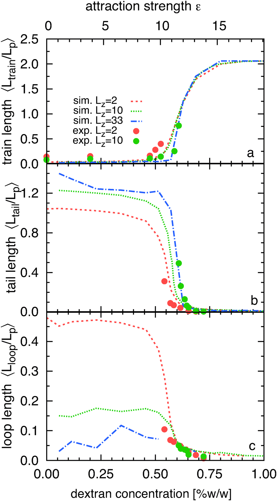 | ||
| Fig. 2 The length of filament trains, tails and loops and their dependence on the attraction strength, ε (or equivalent depletant concentration Cp), averaged over independent configurations and normalized by the filament persistence length Lp. (a) Average train length 〈Ltrain〉/Lp. (b) Average tail length 〈Ltail〉/Lp. (c) Average loop length 〈Lloop〉/Lp. Filled circles correspond to experimental data and lines indicate simulation results. Chamber heights, Lz are specified in the figure legend. The simulation date are scaled onto depletant concentration, Cp, using ε = Cp/C were C = 16.75. | ||
Next we compare experimental data to simulations performed using equivalent molecular parameters. To achieve this the simulation attraction strength, ε, is scaled with a fitting factor C, defined as ε = Cp/C, where Cp is the depletant concentration. The best collapse of simulation data to experiments determines the magnitude of C. We use the same value of C for all our subsequent analyses. In principle, one should be able to compute C from relevant experimental parameters such as the filament surface charge and charge of the glass substrate, the depletant polydispersity and the precise shape of the attraction potential. However, since some of these parameters are difficult to estimate for now we simply use C as a fitting parameter. C = 16.75 yields the best quantitative agreement with the experimental measurements over the entire measurement range (Fig. 2).
In the desorbed and transition regimes the average tail length is considerably larger than the average loop length 〈Ltail〉 > 〈Lloop〉 indicating the dominance of tail over loop fluctuations (Fig. 2b and c). Filament ends are linked to the adsorbed filament segments only on one side, thus they exhibit more pronounced fluctuations and have higher entropy, when compared to loops which are linked to adsorbed segments at both sides. Consequently, for finite sized filaments, the desorbed segments are more likely to be located at the filament ends. To depict this effect clearly, we plot mtrain, mloop, and mtail, the average filament length stored in trains, loops, and tails normalized with L (Fig. 3). These fractions add up to unity. Data plotted in this way confirms that when compared to tails, loops do not play an important role in the desorption of semi-flexible filaments. This is in contrast to longer flexible polymers, where loops dominate the desorption process;24 and also in contrast to stiff rod-like polymers, where loops cannot exist.
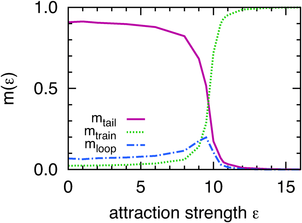 | ||
| Fig. 3 Fraction of the total filament length that is stored in tails, loops and trains as a function of filament-wall attraction strength ε. The simulations were performed for Lz = 2. | ||
It is also possible to elucidate the nature and location of the adsorption transition by examining how the average number of loops 〈Nloop〉 and tails 〈Ntail〉 changes with the filament-wall attractions (Fig. 4). In the strongly adsorbed regime the train length approaches the filament contour length; there is on average only one train and there are very few short loops and tails. Decreasing polymer concentration increases the frequency of configurations with tails and loops. The transition regime can be characterized by a sharp increase in the number of loops and trains. At the transition point 〈Ntail〉 ∼ 2 indicating that essentially all filament configurations have both ends desorbed. Furthermore, 〈Ntail〉 > 〈Nloop〉, indicates that tails dominate over loops, in agreement with previous findings. Finally, below the adsorption transition loops merge with other loops and tails, so that the number of loops decreases and the length of the tails increases. Quantitative agreement between numerical simulations and experiments is obtained using the same scaling parameter, C, used in Fig. 2.
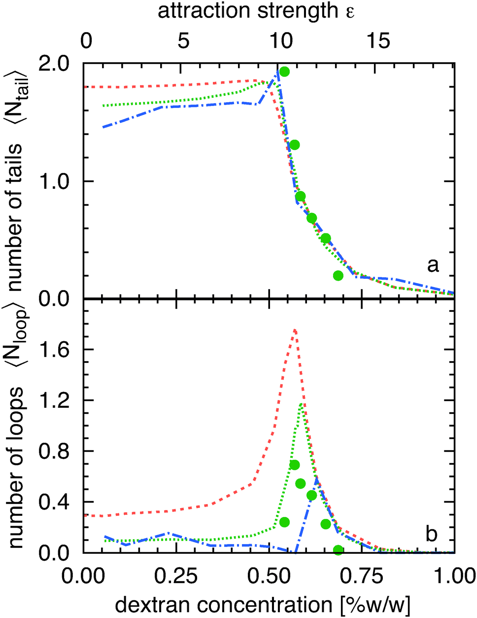 | ||
| Fig. 4 (a) Average number of tails 〈Ntail〉 plotted as a function of the attraction strength, ε (or equivalent the depletant concentration Cp). (b) Average number of loops 〈Nloop〉 as a function of ε. Symbols, lines and color coding is as in Fig. 2. | ||
Increasing polymer confinement decreases the configurational space available to desorbed filaments and thus shifts the adsorption–desorption transition. To explore this effect we have repeated experiments for chambers with two different thicknesses (Fig. 2). For strongly bound filaments, tails, and loops do not extend very far in the bulk and thus cannot interact with the opposite surface. In this regime all measured quantities are independent of confinement. For intermediate attraction strengths, confinement suppresses configurations with tails that extend far into the bulk. Since long tails appear in a configuration either alone or in combination with small loops, removal of these configurations necessarily leads to an effective increase of the average loop size. For weakly bound filaments, the average number of loops decreases strongly but their average size saturates to a constant value which becomes larger with increasing confinement. Changing the number of accessible configurations of the desorbed filament changes the balance between the entropy of the desorbed state and the energy of the adsorbed state, effectively shifting the location of the adsorption/desorption transition to lower attraction strengths. This trend is clear in Fig. 2 where experiments with chambers of different height are shown to be in reasonable agreement with simulations performed with different wall separations.
Given the dominant influence of the tails on the adsorption–desorption transition we investigated in more depth the distribution of tail lengths, p(Ltail) (Fig. 5). In the strong attraction limit the filaments are almost completely adsorbed. Therefore the average tail length is small which leads to a very fast decay of p(Ltail). This distribution can be described with the exponential function
| p(Ltail) ∼ exp[−Ltailζ(Cp)], | (1) |
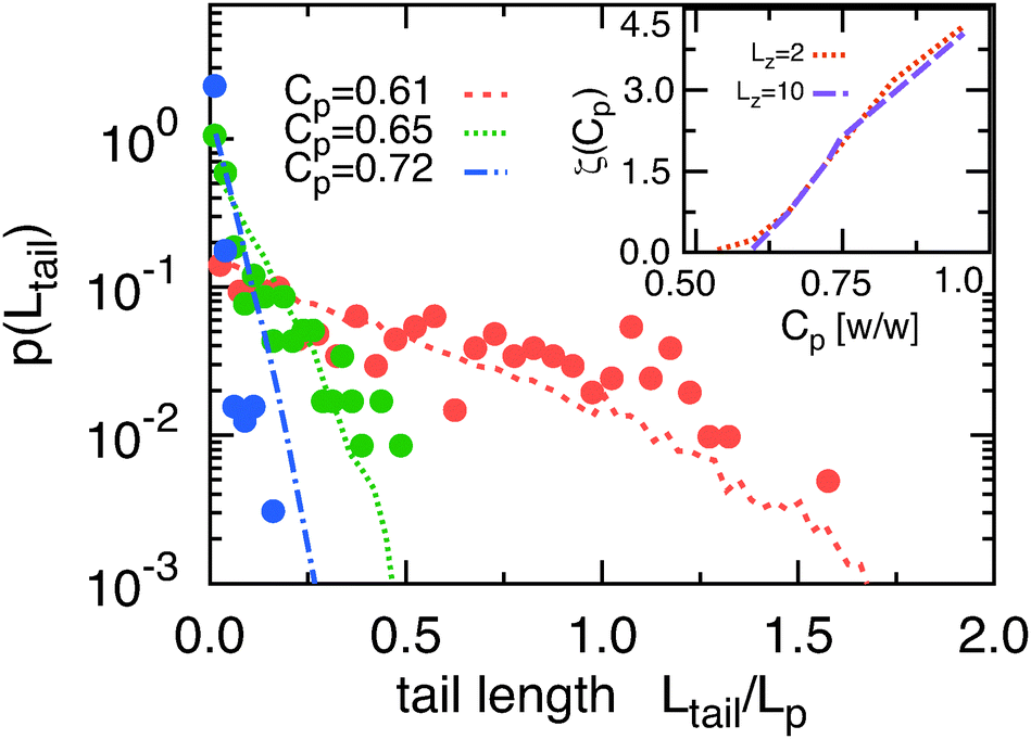 | ||
| Fig. 5 Probability distribution of tail lengths p(Ltail) at three different attraction strengths (depletant concentrations). Filled circles indicate experimental data taken for chambers with Lz = 10 while lines indicate simulations results. Inset: Variation of the inverse decay length ζ for simulations with Lz = 2 and Lz = 10. | ||
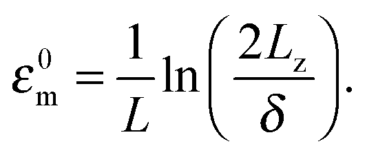
Semi-flexible filaments have more degrees of freedom when compared to rigid filaments. Consequently, confining such filaments onto a wall incurs a larger entropic cost which shifts the adsorption transition to stronger attractions. We investigate this effect by plotting the average fraction of filament length stored in the tails mtail(ε) = 〈Ntail(ε)〉〈Ltail(ε)〉/L for filaments with varying stiffness. In the strongly adsorbed limit mtail(ε) vanishes while in the opposite weak adsorption limit the same quantity approaches a constant value that depends on δ/L (Fig. 6a). For decreasing δ/L this plateau value approaches unity. Following previous work,24 the location of the adsorption transition is identified as the attraction value εm at which half the filament length is desorbed mtail(εm) = 0.5. Increasing the filament flexibility shifts the adsorption transition to larger εm (Fig. 6a). For example, the attraction strength necessary to adsorb a rigid filament ε0m is approximately one order of magnitude lower than the attraction necessary for adsorption of a filament whose persistence length is equal to its contour length. The effect of flexibility on the critical adsorption energy εm can be characterized by the displacement of the attraction at which the adsorption transition occurs as Δεm = εm − ε0m. Plotting Δεm as a function of L/Lp reveals a scaling relationship Δεm ∼ (L/Lp)α where α = 0.37 (Fig. 6b). Simulations for different thickness chambers yields the same power law increase, indicating that Δεm is independent of confinement. Since ε has units of inverse length, a dimensionless quantity ΔεmLβδ1−β can be constructed using the remaining relevant length scales of the problem. The dependency of Δεm on the relevant length scales is further tested by varying L at fixed Lp, varying L/Lp at fixed δ, and simultaneously varying L and δ at fixed Lp. The resulting four data sets collapse onto a single line by using the fitted exponent β = 0.37 (Fig. 6b). Equivalence of α and β implies that Δεm is independent of the filament length. The final result for our scaling relationship is is summarized as
| ΔεmLαpδ1−α ∼ 1. | (2) |
 | (3) |
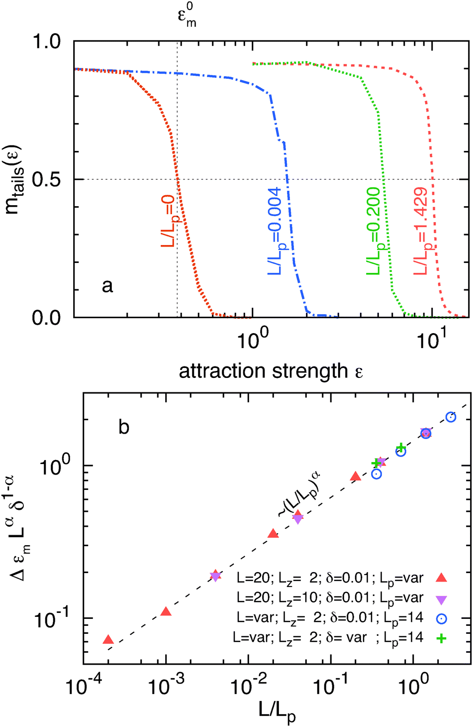 | ||
| Fig. 6 (a) Fraction of the total filament length stored in tails mtail(ε) as a function of the attraction strength ε. Simulations with L = 20 and Lz = 10 for various persistence lengths. The attraction strength ε0m for which half of the infinitely stiff filament is in tails is explicitly indicated. (b) Scaled variation Δεm as a faction of L/Lp with α = 0.37. Symbols correspond to simulations with four sets of parameters indicated in the labels (crosses correspond to (δ, L) = (0.005, 5) and (0.0025, 10)). The dashed line is a fit to a power law dependence (L/Lp)α. | ||
The origin of scaling in Fig. 6b remains unclear. However, it is intriguing that a similar combination of lengths arises in derivation of the Odijk's deflection length, s, which characterizes the fluctuations of filaments confined to a narrow tube.43,51 When the transverse deviation of confined filaments is of the order of the filament spacing D, Odijk's deflection length is defined as s ∼ LαpD1−α with α = 1/3. If we assume that for strongly confined polymers the attraction range of an adsorbed polymer, δ is equivalent to D we find scaling L1/3pδ2/3 which is close to, but not identical to eqn (2). This result suggests that the fluctuations of adsorbed filaments might be analogues to fluctuations of filaments that are confined by an effective tube.
V. Conclusions
In summary, we have combined TIRF microscopy, depletion interactions, semi-flexible F-actin filaments and computer simulations to study the adsorption/desorption of semi-flexible polymers. Real-space visualization enabled us to extract important yet difficult to measure statistics of trains, tails and loops of filaments undergoing the adsorption transition. Our work visually demonstrates the importance of the internal degrees of freedom when considering adsorption of polymers onto a surface. Computer simulations quantitatively agree with experimental results and have enabled us to gain detailed insight in how decreasing the polymer stiffness from a infinitely stiff rod shifts the adsorption transition to larger attraction values. Furthermore, the description of the data in terms of a universal power law dependence opens up the promising possibility of determining the location of the adsorption transition in terms of the polymer length, persistence length, wall separation and attraction range. The similarity of the scaling law with and established theory of polymer confinement in the absence of adsorption is an interesting indication that adsorption and confinement share similar physical grounds. Our theoretical predictions could be further tested in experiments in which the filament persistence length is tuned while keeping all other parameters constant. This might be possible by using filamentous phages, where a point mutations of the major coat protein can tune the filament flexibility by up to 400%.45 The range of the attraction can be modified by using a different size of depleting polymer. From a practical perspective, the surface-induced depletion interactions studied here have been used to assemble diverse soft materials such as extensile microtubule based 2D active nematics, supercoiling actin rings and contractile actin gels.46–49 Similar fluctuations are also important when instead of a surface a filament binds onto another filament. For example, only after accounting for such fluctuations could the effective measured strength of the depletion interaction between a pair of filaments be fitted to a theoretical model.31Acknowledgements
We would like to acknowledge Aggeliki Tsigri, Donald Guu and Dzina Kleshchanok for their collaboration in an initial phase of this work. We thank Jan Kierfeld and Hsiao-Ping Hsu for valuable discussions. DW and ZD acknowledge support of NSF-CMMI-1068566 and NSF-CAREER-0955776. We also acknowledge the use of MRSEC optical microscopy facility which is supported by grants NSF-MRSEC-0820492 and NSF-MRI-0923057.References
- E. Y. Kramarenko, R. G. Winkler, P. G. Khalatur, A. R. Khokhlov and P. Reineker, J. Chem. Phys., 1996, 104, 4806 CrossRef CAS PubMed.
- R. E. Boehm and D. E. Martire, Mol. Phys., 2006, 41, 871 CrossRef PubMed.
- R. R. Netz and J. F. Joanny, Macromolecules, 1999, 32, 9013 CrossRef CAS.
- R. R. Netz and D. Andelman, Phys. Rep., 2003, 380, 1–95 CrossRef CAS.
- A. M. Skvortsov, T. M. Bihrstein and Ye. B. Zhulina, Polym. Sci. USSR, 1976, 18, 2276 CrossRef.
- J. Tang, S. L. Levy, D. W. Trahan, J. J. Jones, H. G. Craighead and P. S. Doyle, Macromolecules, 2010, 43, 7368 CrossRef CAS.
- P. Linse and N. Källrot, Macromolecules, 2010, 43, 2054 CrossRef CAS.
- L. I. Klushin, A. A. Polotsky, H.-P. Hsu, D. A. Markelov, K. Binder and A. M. Skvortsov, Phys. Rev. E: Stat., Nonlinear, Soft Matter Phys., 2013, 87, 022604 CrossRef.
- D. Kuznetsov and W. Sung, J. Phys. II, 1997, 7, 1287–1298 CrossRef CAS.
- A. C. Maggs, D. A. Huse and S. Leibler, Europhys. Lett., 1989, 8, 615–620 CrossRef CAS.
- T. M. Birshtein, E. B. Zhulina and A. M. Skvortsov, Biopolymers, 1979, 18, 1171–1186 CrossRef CAS PubMed.
- A. N. Semenov, J. Bonet-Avalos, A. Johner and J. F. Joanny, Macromolecules, 1996, 29, 2179 CrossRef CAS.
- C. C. van der Linden, F. A. M. Leermakers and G. J. Fleer, Macromolecules, 1996, 29, 1172 CrossRef CAS.
- C. A. J. Hoeve, E. A. DiMarzio and P. Peyser, J. Chem. Phys., 1965, 42, 2558 CrossRef CAS PubMed.
- A. Silberberg, J. Phys. Chem., 1962, 66, 1872 CrossRef CAS.
- M. A. Cohen-Stuart, T. Cosgrove and B. Vincent, Adv. Colloid Interface Sci., 1986, 24, 143–239 CrossRef CAS.
- L. Auvray and J. P. Cotton, Macromolecules, 1987, 20, 202–207 CrossRef CAS.
- H.-P. Hsu and K. Binder, Macromolecules, 2013, 46, 8017–8025 CrossRef CAS.
- T. T. Perkins, D. E. Smith and S. Chu, Science, 1994, 264, 819–822 CAS.
- T. T. Perkins, S. R. Quare, D. E. Smith and S. Chu, Science, 1994, 264, 822–826 CAS.
- J. Käs, H. Strey and E. Sackmann, Nature, 1994, 368, 226–229 CrossRef PubMed.
- B. Maier and J. O. Radler, Phys. Rev. Lett., 1999, 82, 1911–1914 CrossRef CAS.
- C. Rivetti, M. Guthold and C. Bustamante, J. Mol. Biol., 1996, 264, 919–932 CrossRef CAS PubMed.
- H.-P. Hsu and K. Binder, Macromolecules, 2013, 46, 2496–2515 CrossRef CAS.
- P. A. Sánchez, J. J. Cerda, V. Ballenegger, T. Sintes, O. Piro and C. Holm, Soft Matter, 2011, 7, 1809 RSC.
- F. Gittes, B. Mickey, J. Nettleton and J. Howard, J. Cell Biol., 1993, 120, 923–934 CrossRef CAS.
- F. R. Senti, N. N. Hellman, N. H. Ludwig, G. E. Babcock, R. Tobin, C. A. Glass and B. L. Lamberts, J. Polym. Sci., 1955, 17, 527–546 CrossRef CAS PubMed.
- A. D. Dinsmore, A. G. Yodh and D. J. Pine, Nature, 1996, 383, 239–242 CrossRef CAS PubMed.
- S. Asakura and F. Oosawa, J. Chem. Phys., 1954, 22, 1255 CAS.
- D. Axelrod, Methods Enzymol., 2003, 361, 1–33 CAS.
- A. W. C. Lau, A. Prasad and Z. Dogic, Europhys. Lett., 2009, 87, 48006 CrossRef.
- T. Sanchez and Z. Dogic, Methods Enzymol., 2013, 524, 205–226 CAS.
- J. D. Pardee and J. A. Spudich, Methods Enzymol., 1982, 85, 164–181 CAS.
- E. M. De La Cruz and T. D. Pollard, Biochemistry, 1996, 35, 14054–14061 CrossRef CAS PubMed.
- C. Picart and D. E. Discher, Biophys. J., 1999, 77, 865–878 CrossRef CAS.
- See ESI‡ for TIRF and Epi-fluorescence movies obtained in the desorbed and the transition regimes.
- H.-P. Hsu, W. Paul and K. Binder, Europhys. Lett., 2010, 92, 28003 CrossRef.
- H.-P. Hsu, W. Paul and K. Binder, Europhys. Lett., 2011, 95, 68004 CrossRef.
- M. Doi and S. F. Edwards, The theory of polymer dynamics, Oxford University Press, 1986 Search PubMed.
- J. Kierfeld and R. Lipowsky, Europhys. Lett., 2003, 62, 285 CrossRef CAS.
- M. Lal, Mol. Phys., 1969, 17, 57 CrossRef CAS PubMed.
- N. Madras and A. D. Sokal, J. Stat. Phys., 1988, 50, 110 CrossRef.
- T. Odijk, Macromolecules, 1983, 16, 1340 CrossRef CAS.
- M. Möddel, W. Janke and M. Bachmann, Macromolecules, 2011, 44, 9013–9019 CrossRef.
- E. Barry, D. Beller and Z. Dogic, Soft Matter, 2009, 5, 2563–2570 CAS.
- T. Sanchez, D. T. N. Chen, S. J. DeCamp, M. Heymann and Z. Dogic, Nature, 2012, 491, 431–434 CrossRef CAS PubMed.
- F. C. Keber, E. Loiseau, T. Sanchez, S. J. DeCamp, L. Giomi, M. J. Bowick, M. C. Marchetti, Z. Dogic and A. R. Bausch, Science, 2014, 345, 1135–1139 CrossRef CAS PubMed.
- M. P. Murrell and M. L. Gardel, Proc. Natl. Acad. Sci. U. S. A., 2012, 109, 20820–20825 CrossRef CAS PubMed.
- T. Sanchez, I. M. Kulic and Z. Dogic, Phys. Rev. Lett., 2010, 104, 098103 CrossRef CAS.
- Hsu and Binder have characterized the distribution function of loops for grafted long semi-flexible polymers finding a behavior consistent with a power law decay (see Fig. 20 in ref. 18).
- T. Odijk, Phys. Rev. E: Stat., Nonlinear, Soft Matter Phys., 2008, 77, 060901 CrossRef.
Footnotes |
| † 61.30.Hn, 61.30.Dk, 82.70.Dd. |
| ‡ Electronic supplementary information (ESI) available. See DOI: 10.1039/c5sm01457c |
| This journal is © The Royal Society of Chemistry 2015 |