Glassy dynamics of a polymer monolayer on a heterogeneous disordered substrate

Abstract

We present molecular dynamics simulations of a polymer monolayer on randomly functionalized surfaces that are characterized by different fractions of weakly and strongly attractive sites. We show that the dynamics slow-down upon cooling resembles that of a strong glass-forming liquid. Indeed, the mean-square displacements show an increasingly lasting subdiffusive behaviour before the diffusive regime, with signs of Fickian yet not Gaussian diffusion, and the dynamic correlation functions exhibit a stretched exponential decay. The glassy dynamics of this relatively dilute system is dominated by the interaction of the polymer with the substrate and becomes more marked when the substrate composition is heterogeneous. Accordingly, the estimated glass transition temperature shows a non-monotic dependence on surface composition, in agreement with previous results for the activation energy and with an analysis of the potential energy landscape experienced by the polymer beads. Our findings are relevant to the description of polymer–surface adhesion and friction and the development of polymer nanocomposites with tailored structural and mechanical properties.

---

1 Introduction

The interaction of polymers with solid substrates is relevant for a wide range of problems and applications, including adhesion,¹ friction² and nanocomposites^3,4 (in the latter case, the interaction occurs at the internal interface, between the polymer matrix and the nanoparticles). In addition, polymer brushes can play an important role in the adsorption and the assembly of nanoparticles at liquid interfaces.^5,6 Similar problems occur everywhere in molecular biology and living organisms, as exemplified by biocomposites (e.g. bone), biomineralization and biopolymer-cell recognition. Due to their pervasiveness and intrinsic interest, these issues have been extensively studied since the early days of polymer physics. It is now well established that the interaction of a single chain or a polymer melt with a solid surface is usually accompanied by major changes in their statistical conformation and dynamics – see ref. 7–10, for example – and that “quenched” disorder in the polymer sequence (copolymers) or on the surface (chemical heterogeneity and roughness) can also play a major role.^11–13

One of the most important indicators of the properties and potential use of a polymeric material is its glass transition temperature, T_g.¹⁴ A bulk amorphous polymer is said to be rubbery above its T_g, glassy below it. The neighbourhood of a solid substrate may either increase or decrease the polymer T_g with repect to the bulk value, depending on the nature and strength of the polymer–substrate interactions.^15–23 Similar effects are also seen in nanocomposites,²⁴ where they are actually amplified due to the high extension of the interfacial region between the polymer and the nanoparticles.^3,4,25 Several aspects of the mechanical properties of elastomeric nanocomposites (filled rubbers) can indeed be interpreted on the basis of a two-phase model, whereby the polymer chains within a few nanometres from the nanoparticles are glassy, whereas those away from them have a rubbery response, similar to that of the bulk, unfilled polymer. While the fundamental understanding of the glass transition is still a major open issue in condensed matter,²⁶ it is also interesting to investigate the behaviour of glassy systems in these technologically relevant situations.

Many glass forming materials, such as molecular liquids, colloids and polymer melts, can be suitably modeled by systems of spheres interacting by a combination of Lennard-Jones and harmonic or FENE (Finitely Extensible Non-linear Elastic) potentials, respectively representing the bonded and non-bonded interactions.²⁷ For these systems, glassy dynamics typically emerges upon cooling at rather high densities. Models of bulk and confined polymer melts (in 3D and quasi-2D, respectively) approaching the glass transition temperature are usually equilibrated at zero or positive pressures, yielding monomer number densities around ρ ≃ 1 or slightly larger.^28,29 Here we show that the glassy dynamics can be relevant for polymer chains adsorbed on solid substrates – a common situation for many of the applications mentioned above – even in the case of a rather dilute system. Previous simulation work demonstrated that glassy behaviour can be brought about also by strong chemisorptive interactions, which often occur on metallic surfaces,³⁰ and that there can be significant differences between the glassy polymer dynamics on a ideally flat substrate and on an atomically structured one.³¹ Following a previous work by one of us,³² in this paper we have carried this idea one step further by considering the emergence of glassy dynamics on a chemically heterogeneous surface. For comparison, we have also investigated the behaviour of the same polymer system on a homogeneous substrate, which can be either perfectly smooth or have some atomic-scale roughness. We find that the polymer on the flat substrate has a trivial behaviour, with weak temperature dependence and no glassy dynamics (see the Appendix). The glassy behaviour appears only on a structured substrate and is enhanced by heterogeneity. Upon cooling, the mean-square displacement of the polymer chains displays an increasingly lasting subdiffusive behaviour before entering the diffusive regime, with the distribution of particle displacements highlighting a Fickian yet not Gaussian diffusion. The autocorrelation of the Rouse Normal Modes decays as a stretched exponential function, and, overall, the dynamics resembles that of strong glass-forming liquids. This enables us to estimate the glass transition temperature of the systems, evidencing a non-monotonic dependence on the substrate composition. This feature can be related to the characteristics of the potential energy landscape experienced by the polymer segments.

2 Model and methods

2.1 Model

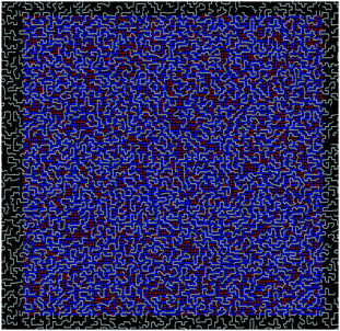
We performed equilibrium molecular dynamics (MD) simulations of the model introduced in ref. 32 and 33. Briefly, the systems contain several flexible polymer chains of N “P” beads, connected by harmonic springs and deposited on a solid surface (see Fig. 1). The substrate consists of a single layer of two types of atoms, strongly “S” and weakly “W” interacting, rigidly arranged on a square planar lattice, at a height z = 0.0. Substrates characterized by different compositions were generated by randomly assigning the type to the surface atoms, with probability f for the S atoms and 1 − f for the W ones. In particular, we sampled the whole range of surface compositions, focussing on five evenly spaced values of f, i.e. f = 0.00, 0.25, 0.50, 0.75, and 1.00. Two additional values in between the latter, f = 0.12, 0.88, have also been considered for some analysis. In our model, all non-bonded interactions (between two particles p and q) are described by truncated and shifted Lennard-Jones (LJ) potentials:^34,35

V^LJ_PQ(r) = 4ε_PQ[(σ/r)¹² − (σ/r)⁶] − V_PQ (1)

if r < r_PQ, V^LJ_PQ(r) = 0 otherwise. Here the subscript Q is the type of particle q (i.e., P, W or S; particle p is always of P type, as indicated), σ is the hard-core diameter of all atoms (P, W, and S), ε_PQ is the interaction strength (LJ well depth), r_PQ is a cutoff distance and V_PQ an energy shift factor which exactly zeroes the potential at the cutoff, thus preserving its continuity over all distances. The interaction strength between polymer beads and strong sites is twice the other strengths, i.e. ε_PP = ε_PW = ε and ε_PS = 2ε. All polymer surface interactions are truncated at a cutoff distance of r_PW = r_PS = 2.5σ, whereas the polymer–polymer interactions are truncated at r_PP = 2^1/6σ ≃ 1.122σ to produce a purely repulsive potential. With this choice the chains adopt an essentially two-dimensional “pancake” conformation. Units are reduced so that σ = m = ε = k_B = 1, where m is the mass of all atoms and k_B is the Boltzmann constant. Periodic boundary conditions were adopted in the directions parallel to the surface (x and y). We used n = 450 chains of length N = 16 and a substrate of side L = 100, resulting in a density ρ = Nn/L² = 0.72, and investigated a temperature range T ∈ [0.4, 1.2]. Temperature was controlled by a standard Langevin thermostat,³⁶ and the resulting equations of motion were integrated with a (reduced) timestep Δt = 0.01. The simulations were carried out with the COGNAC code.³⁹

Fig. 1 Model system. An illustration of the investigated system with f = 0.75, at T = 0.7. The P chains are white, W surface sites red, S surface sites blue. The black area corresponds to different replicas of the system's unit cell, with periodic boundary conditions.

A small constant force f_z = −0.1 (in LJ units) was applied to all the P beads along the z direction, gently pressing them against the underlying surface to prevent any detachment and long-range “jumps” of the chains. This possibility has been seen experimentally under appropriate conditions^37,38 and sometimes we also observed it in a preliminary set of simulations at the highest temperatures (T ≥ 1.0). Thus, the force was applied in order to simplify the analysis and interpretation of the MD results, by preventing these rare adsorption/desorption events and concentrate exclusively on the planar dynamics of the adsorbed chains. The force itself does not have a special physical meaning, but we note that a similar effect could have been obtained by running the MD simulations in an extremely narrow slit (width comparable to the chains' radius of gyration).

2.2 Mapping

To connect our results with real material properties, we adopted an approximate mapping based on the following monomer properties:⁴⁰ diameter σ₀ = 0.7 nm, mass m₀ = 100 N_A⁻¹ g, and interaction energy ε₀ = 0.04 eV, where N_A is the Avogadro's number. With this mapping, each bead would roughly correspond to 6–7 carbon atoms in a real polymer chain. This leads to resonable, semiquantitative results for typical polymer properties. In particular, the characteristic time and temperature of our bead-and-spring model are t₀ = (m₀/ε₀)^1/2σ₀ = 3.56 ps and T₀ = ε₀/k_B = 464.35 K, where k_B is the Boltzmann constant. These will be used to extrapolate the simulation results to experimental time and temperature scales in Section 3.3.

3 Results

3.1 Diffusion

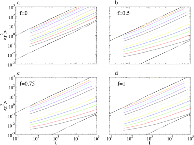
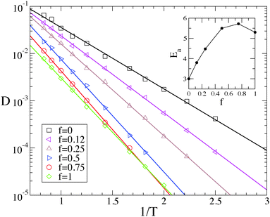
We start by illustrating the diffusive properties of the system. The double logarithmic plots in Fig. 2 show the mean-square displacements (MSD's) 〈r²(t)〉 of the polymers' center of mass for different temperatures and surface compositions. At f = 0 (panel a) and high temperature the motion is diffusive from the beginning, as 〈r²(t)〉 ∝ t within our temporal resolution (MD snapshots were saved at intervals Δt = 50, in our reduced LJ units). At lower temperature, the long-time diffusivity decreases, and the diffusive regime is preceded by a sub-diffusive one which becomes increasingly lasting upon cooling. This behaviour is more marked at higher values of f (panels b, c and d), inasmuch as at low temperature the diffusive regime is not recovered within the simulated time. This resembles the intermediate time plateau which is observed in the MSD of glass-forming materials.⁴² This distinctive property of glass-formers is typically ascribed to the particle crowding and to the consequent cage-jump motion, recently investigated in detail in simulations of molecular liquids^43–45 and of concentrated polymer melts,²⁸ and in experiments on colloidal glasses.⁴⁶ In our case, the primary cause of transient confinement is not the particle crowding, but rather the interaction with the substrate. This not only slows down the polymer motion as a result of the mutual affinity, but also creates the heterogeneous energy landscape shown in Fig. 9. In the case of a single-species substrate (f = 0 and f = 1), this heterogeneity merely arises from the surface's atomic discreteness. Conversely, at intermediate values of f, heterogeneity is enhanced by the presence of S and W particle clusters of different sizes and shapes and therefore it might also be related to the random percolation properties of the substrate. As a matter of fact, accurate inspection of Fig. 2 reveals that at the lowest temperatures the sub-diffusive regime is longer for f = 0.75 than for f = 1, suggesting that heterogeneity does play an important role.

Fig. 2 Mean square displacement as a function of time, for T = 1.2, 1.1, 1.0, 0.9, 0.8, 0.7, 0.6, 0.55, 0.5, 0.45, and 0.4 from top to bottom. Different panels report different values of f, as indicated. Dashed lines are guides to the eye of slope 1.

The last statement becomes more evident by focussing on the diffusion constant D, defined by the long-time limit of the MSD: . Fig. 3 shows that its temperature dependence is well described by the Arrhenius law,

D ∝ exp(−E_a/T), (2)

characterizing activated processes in a static energy landscape. The present data do not suggest any crossover to a super-Arrhenius behaviour typical of fragile glass-formers (including bulk polymers), in agreement with the scarce relevance of cooperative effects in our dilute system (see Appendix). The estimated activation energy E_a, shown in the inset of Fig. 3, has a maximum at f = 0.75, where the diffusivities vanish faster. This confirms earlier findings by one of us,³² the final numerical values being only slightly different since here we have been more careful to exclude the sub-diffusive regime and some truly glassy data points from the fits.⁴⁷ The maximum in the activation energy results from the combined effects of interaction strength and heterogeneity. The former increases linearly between f = 0.00 and f = 1.00, while the latter is maximum between f = 0.50 and f = 0.75, depending on the statistical quantity used to describe it, as we discuss later (see Section 3.4).

Fig. 3 Diffusion constant D as a function of 1/T and at different values of f, as indicated. Solid lines are Arrhenius fits to the data: D ∝ exp(−E_a/T). Inset: Activation energy E_a as a function of f.

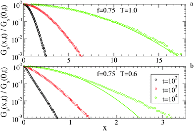
As a final characterization of the diffusion properties, we investigate the distribution of particle displacements, i.e. the van Hove function,

G_s(x,t) = 〈δ[x − |X_i(t) − X_i(0)|]〉, (3)

where X_i(t) is the center-of-mass position of polymer i at time t along a given direction and the brackets indicate an ensemble average. As typical of Brownian systems, at short times G_s(x,t) decays exponentially and progressively evolves into a Gaussian as time passes. Fig. 4a shows that this crossover is fully manifested at high temperature, even for f = 0.75. Fig. 4b, instead, refers to the lowest temperature where the diffusive regime can still be observed within the simulated time. In this case, the van Hove function retains the exponential tails at the longest available time, i.e. well after the system enters the diffusive regime. This is a typical manifestation of the Fickian yet non-Gaussian diffusion found also in glass-formers and other soft materials.^37,48

Fig. 4 Particle displacement distribution divided for its maximum G_s(x,t)/G_s(0,t) at f = 0.75, at different times and temperatures, as indicated. Solid lines are Gaussian fits exp(−x²/2λ²(t)) to the data at the longest time.

3.2 Conformational relaxation

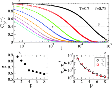
The glassy dynamics of the polymer chains is reflected also by their slowed-down conformational relaxation. This has been investigated via the autocorrelation function C_p(t) = 〈Q_p(0)·Q_p(t)〉 of the Rouse Normal Modes (RNMs):⁴⁹where r_j(t) is the position of monomer j at time t and p = 1, 2, …, N − 1 is the mode index (the polymer center-of-mass formally corresponds to mode p = 0). We first focus on the surface producing the most glassy dynamics, f = 0.75. Fig. 5a shows C_p(t) for different values of p at temperature T = 0.7, where the slowest mode still relaxes over the simulated time. The decay is not consistent with a simple exponential, as predicted by the original Rouse model, but it is well described by a stretched exponential,

C_p(t) ≃ exp[−(t/τ^s_p)^β] (5)

with β ≤ 1. This rather general form of relaxation in equilibrium supercooled liquid has been related to heterogeneous dynamics,⁵⁰ while also compressed exponentials (β ≥ 1) can be typical of non-equilibrium aging glasses.⁵¹ The predictions of the Rouse model are respected in a melt of short polymer chains, where excluded-volume, entanglement and hydrodynamic interactions are negligible.⁴⁹ Away from these conditions, “stretching” of the Rouse modes may occur for a variety of reasons, such as the approach to the glass transition,⁵² dynamic asymmetries in blends of flexible and stiff chains,⁵³ geometrical constraints due to randomly dispersed nanoparticles.⁵⁴ In their theoretical analysis of the Langevin dynamics of a polymer chain in a random potential, Vilgis and coworkers^13,55 also predicted that the stretching of the Rouse modes should be accompanied by an incomplete relaxation (i.e., whenever β < 1, where f_p > 0 is the so-called non-ergodicity parameter for mode p). Here, however, we find that this is not the case, possibly because the disorder strength in our model is not high enough (it could be increased by including more surface types, with a greater disparity in interaction energy).

Fig. 5 (a) RNM autocorrelation function C_p(t) at f = 0.75, T = 0.7 and p = 1, 2, …, 8, from right to left. Solid lines are stretched exponential fits to the data, C_p(t) = exp[−(t/τ^s_p)^β]. (b) Exponent β as a function of p. (c) Fitted τ^s_p and measured τ_p relaxation time (C_p(τ_p) = 1/e) as a function of p. The solid line is a fit to the data, τ_p ∝ p^−a (a = 2.8 ± 0.08).

Fig. 5b shows that β is smaller at larger p (i.e., for more localized modes), indicating a more heterogeneous relaxation, while the RNM relaxation times increase by more than two orders of magnitude, as reported in Fig. 5c. The decrease of β at larger p is reflected in the deviation from the quadratic scaling τ_p ∝ p⁻² predicted by the Rouse model. Indeed, we find a quite strong deviation τ_p ∝ p^−a, with a = 2.8 ± 0.08. This agrees qualitatively with the generalized Langevin Model, which predicted a = 2/β under some simplifying assumptions.⁵³ Incidentally, note the good agreement between the relaxation times obtained from the fits (τ^s_p, see again eqn (5)) and those measured on the relaxation curves (τ_p, where C_p(τ_p) = 1/e). The RNM relaxation properties are rationalized by considering that mode p is associated with a typical length-scale, as it describes the collective motion of chain sections containing N/p beads. The most collective modes (small p) require longer times to relax (large τ_p), but the heterogeneity of the surface is averaged on the corresponding length scale, becoming less relevant for the polymer dynamics (β ≃ 1).

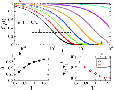
Fig. 6a shows the most collective mode C₁(t) at different temperatures. At very low temperature the dynamical correlation function does not relax on the simulated timescale, precluding a reliable fit to the data. At larger T, β increases, as shown in Fig. 6b, and becomes 1 in the high temperature limit, where exponential decay is recovered. The very good agreement between τ^s₁ and τ₁ is confirmed (see Fig. 6b). Although less markedly, a similar scenario holds for different values of f.

Fig. 6 (a) C₁(t) at f = 0.75, p = 1 and T = 1.2, 1.1, 1.0, 0.9, 0.8, 0.7, 0.6, 0.5, and 0.4 from left to right. At low temperature the correlation function does not decay within the simulated time. Solid lines are stretched exponential fits to the data, C_p(t) = exp[−(t/τ^s_p)^β]. (b) Exponent β, (c) τ^s_p and τ_p as a function of T.

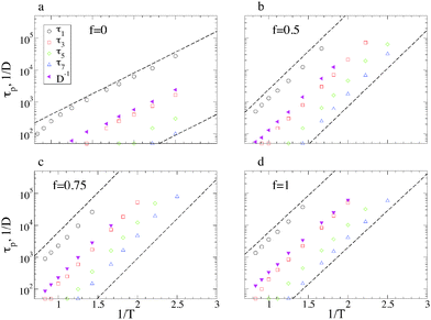
The different panels of Fig. 7 show the temperature dependence of the RNM relaxation times τ_p(T). The inverse diffusion constant D⁻¹ is reported for comparison. As distinctive of strong glass-formers, the relaxation times follow the Arrhenius behaviour of eqn (2), a kind of Stokes–Einstein relation being valid:

τ_p(T) ∝ D⁻¹(T). (6)

Fig. 7 RNM relaxation times τ_p for different values of p, and inverse diffusion constant D⁻¹ as a function of the inverse temperature. The different panels report different values of f, as indicated. Dahed lines are Arrhenius guides to the eye ∝ exp(−E_a/k_BT).

3.3 Glass transition temperature

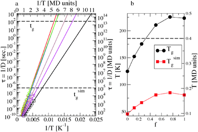
The glass transition temperature T_g can be defined as the temperature where the shear relaxation time exceeds a given time threshold, compatibly with the available observation timescale. In experiments this threshold is conventionally set at t_g = 10²–10³ s,⁵⁶ while in simulations it is constrained by the CPU time, resulting in simulated times t^sim_g substantially short compared to experiments.

We obtain a rough estimation of the characteristic relaxation time from the relation τ = D⁻¹.⁵⁷Fig. 2 clarifies that the equilibrium systems become diffusive for t < τ and that 〈r²(τ)〉 ≃ 1. Thus τ is the time required by a chain to diffuse a distance of the order of the atomic spacing in the underlying surface, which for our short polymers is also of the order of its radius of gyration. In analogy of the mentioned definition of T_g and of the approach recently used in ref. 23, we can obtain by extrapolating the temperature at which τ would reach an arbitrarily large threshold, exploiting the robust Arrhenius behaviour found on the investigated timescale. By using the mapping described in Section 2.2, we convert the reduced MD units in the experimental ones and obtain T_g from τ(T_g) = t_g = 100 s. This procedure is illustrated in the two panels of Fig. 8, where the corresponding MD units are also reported on the axes. Besides, it is worth noticing that any (reasonably) different choice of the time threshold or of the mapping scheme has a negligible effect on T_g. Differentiating the Arrhenius law, it results dT_g ∝ exp(−E_a/T_g)dt_g and thus a change in t_g is exponentially weakened, resulting in a very small change in the estimated glass transition temperature. For comparison, we also extrapolate T^sim_g, which is akin to a “glass transition temperature” on the simulated time: τ(T^sim_g) = t^sim_g, where t^sim_g ≃ 10⁻⁵ s after the mapping.

Fig. 8 (a) Relaxation time τ = D⁻¹ as a function of inverse temperature and at different values of f, as indicated. The horizontal dashed lines mark the typical experimental observation time t_g and the simulation duration t^sim_g, respectively. These timescales are used to define the experimental T_g and numerical T^sim_g glass transition temperatures, from the intercepts with the Arrhenius fits (solid lines). (b) T_g and T^sim_g as a function of f. The horizontal dashed line marks the lowest investigated temperature.

Fig. 8 shows T_g and T^sim_g as a function of the surface composition. Similar to the activation energy, both temperatures have a maximum at around f = 0.75. We note that T^sim_g is higher than the lowest investigated temperature, for f > 0.25. This is consistent with the behaviour found for the MSD, which at low temperature and large f no more reaches the diffusive regime within the simulated time (see Section 3.1). Finally, we point out that glass transition temperatures of the order of 50–100 K are low in comparison with typical elastomer values (200–250 K), but this is understandable considering that ours is a dilute system with purely repulsive polymer–polymer interactions, and there are no conformational barriers in our bead-and-spring model.

3.4 Potential energy landscape

We rationalize the system dynamics presented above, investigating the potential energy landscape seen by the polymer beads. In earlier publications by one of us,^32,33 we did this by sampling their adsorption energies, placing a P bead at a fixed height above the centre of the squares formed by four neighbouring surface atoms. The resulting histograms demonstrated that (a) the average polymer–surface interaction energy increases linearly from f = 0 to f = 1, and (b) the broadest distribution of these energies is obtained for f = 0.5, which can thus be considered the “most disordered” substrate. However, this procedure does not yield any information about the energy barriers separating the absorption energy minima, which are important for the dynamics of the adsorbed polymers. Here we provide a more extensive characterization, including information about the energy barriers to diffusion.

Fig. 9 shows some representative plots of the potential energy of a P bead, as it slides horizontally along a short section of five different surfaces. These plots were obtained by running MD simulations at a very low temperature (T = 0.01), constraining the y coordinate of the bead at a value corresponding to a row of absorption minima, and its x coordinate to move at a constant velocity v_x = 1.0 (see the inset in Fig. 9). Thus, the z coordinate of the bead is the only degree of freedom in these simulations, and this oscillates up and down as the bead moves from a minimum, to a maximum (actually, a transition state), to the next minimum.⁴¹ As expected, the two homogeneous surfaces have a periodic potential energy pattern, the energies for f = 1 being twice as large as those for f = 0. Instead, those for f = 0.25, 0.50, and 0.75 are non-periodic and irregular, reflecting the randomness in the chemical identity (W or S) of the underlying atoms. The average energy appears to decrease (i.e., to become more negative) as f increases, but it is hard to draw further conclusions about the “roughness” in the potential energy landscape by visual inspection of these plots.

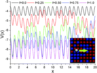Fig. 9 Potential energy scans. Representative potential energy profiles, for a P bead sliding along surfaces with different f's, as shown in the inset.

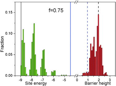
Fig. 10 shows the histograms of the energies of the minima (negative values, in green) and of the barriers separating these minima (positive values, in red), as obtained by scanning across a surface with f = 0.75. The information contained in the former is essentially equivalent to that given in earlier papers.^32,33 It shows that on a random, heterogeneous surface there can be different types of absorption sites. The distribution can be rather broad, but the energies are always comprised between those on the f = 0 and f = 1 surfaces. Instead, the information in the red histogram is new and demonstrates that on this surface there is also a broad distribution of energy barriers. Unlike the energy minima, these can be both smaller and larger than those for f = 0 and f = 1, respectively. In particular, the large fraction of high energy barriers can be expected to have a significant effect on the polymer dynamics on this surface.

Fig. 10 Potential energy histograms. Histograms of the energies of the minima (in green) and of the barriers separating these minima (in red), for the surface with f = 0.75. The vertical lines represent energies of the minima (continuous) and of the barriers (dashed) of the homogeneous surfaces, with f = 0 (blue) and f = 1 (black).

Table 1 collects some significant statistical properties, for all the studied surfaces. The mean value of the potential 〈V〉 changes linearly with f, and so does the mean barrier height 〈V_b〉. Instead, the standard deviation σ_V (=〈(V − 〈V〉)²〉^1/2) is maximum for f = 0.5, confirming that this is the “energetically roughest”. Notice that the values of 〈V〉, 〈V_b〉 and σ_V for the f = 1 surface are equal to twice those for the f = 0 one, suggesting a linear relationship between activation energy and surface–polymer interaction strength in the homogeneous case. Finally, we give in Table 1 also the fraction b_f of energy barriers which are strictly larger than that on the most strongly interacting surface, with f = 1. This appears to achieve its maximum between f = 0.75 and f = 0.88, where more than one in four monomer “hops” involves such a large energy requirement. We conclude that the latter is probably the most significant descriptor of the surfaces, as it is the one that correlates best with the polymer dynamics described in the previous sections.

Table 1 Potential energy statistics. Properties of the potential energy landscapes, for different values of f. 〈V〉 and σ_V are the mean and standard deviation of the potential energy. 〈V_b〉 is the mean barrier height. b_f is the percentage of energy barriers which are larger than that on the surface with f = 1

f	〈V〉	σ V	〈Vb〉	b f (%)
0.00	−3.97	0.34	0.95	0.0
0.12	−4.53	0.71	1.12	1.6
0.25	−4.98	0.85	1.23	4.3
0.50	−5.97	1.00	1.49	14.6
0.75	−6.97	0.93	1.73	27.6
0.88	−7.51	0.84	1.86	26.9
1.00	−7.97	0.69	1.97	0.0

---

In the present model, there are no correlations in the positions of the surface sites. However, one could also think of situations with S-rich and W-rich “patches” on the surface. The composition, the size and the shape of these patches would clearly be important and affect the chain dynamics through the potential energy landscape. For example, considering the situation with f = 0.50, one could gradually switch from broad monomodal (randomly intermixed case) to bimodal distributions of both the energy minima and the barriers (fully segregated case). What would be the consequences on the dynamics of an absorbed chain? In principle, many situations are possible. Considering for example a weakly segregated situation, the chains would clearly tend to populate the S-rich patches, thus feeling an “effective composition” corresponding to a locally enhanced value of f (0.75, say). The result would be a shift of the maxima in the effective activation energy and T_g, to a smaller f.

4 Conclusion

We have shown that the dynamics of a molecularly thin polymer layer on a solid substrate becomes glassy upon cooling, in spite of the fact that cooperative effects are not an intrinsic property of the investigated polymer system, which is indeed quite dilute. Instead, such a slow dynamics is induced by the affinity for the surface and by the structural heterogeneity of the latter, which in our model are both controlled by the fraction f of strongly interacting sites. Upon increasing the affinity, the polymer motion becomes slower as in a more viscous medium, while the structural heterogeneities create a corrugated energy landscape which also interferes with diffusion. The glassy dynamics is more marked at f = 0.75, as a sort of compromise between interaction strength and heterogeneity. In this respect, the most relevant description of the potential energy landscape appears to be the fraction of large barriers, where here “large” means exceeding the value for the most strongly interacting surface. The spatial extension of the polymer chains tends to average out the effects of heterogeneity, but never completely, as polymer diffusion always proceeds through a series of discrete hopping events involving individual monomers or short chain sections.

The Arrhenius behaviour of the relaxation time suggests that activated events are not cooperative at all or that their size is temperature independent. In order to clarify this issue we plan to investigate the segmental dynamics for different chain length N. This includes not only the behaviour of much longer polymer chains, but also N = 1, i.e. soft spheres. This simpler system should allow us to identify more precisely the relationship between structural heterogeneity of the substrate and dynamical heterogeneity of the diffusing particles. It would also be interesting to extend these studies to confined and nanoparticle-filled polymer melts. With an increased polymer density, we would expect to observe a growth in cooperativity upon cooling, with fragile glass behaviour eventually taking over the strong glass behaviour observed in the present case. Another possibility is to examine surfaces with different geometrical features (hexagonal instead of square planar arrangements of atoms, say), to enhance the surface heterogeneity (using ε_S/ε_W > 2), or to introduce some “patchiness” on the surfaces (correlations in the positions of W and S sites). In principle, each of these variations should produce a shift in the surface composition corresponding to the maxima in E_a and T_g.

Appendix: dynamics on a smooth surface

In order to better appreciate the dynamic effects of the heterogeneous surfaces described in the main text, here we discuss the behaviour of the same polymer system but interacting with a perfectly smooth surface. In this case, the potential energy of a polymer bead interacting with a surface at z = 0 is obtained by integrating the pairwise Lennard-Jones interactions over all the atoms making up the wall, and is a function only of its z coordinate:⁵⁸ The number density of wall atoms (ρ_w) and their Lennard-Jones parameters (ε_w and σ_w) have all been taken equal to unity, to be comparable with the f = 0 discrete surface.

Fig. 11a shows that the mean square displacement is diffusive at short time, even at very low temperature, without the intermediate time subdiffusive behaviour found for the discrete surfaces (cf.Fig. 2). Fig. 11b shows that the decrease of the diffusion constant upon cooling is compatible with a power law, D(T) ∝ T^b (b = 1.18 ± 0.05), i.e. much slower than the Arrhenius behaviour found for the heterogeneous surfaces (cf.Fig. 3). The decay with time of the RNM autocorrelation functions is fully compatible with that predicted by the Rouse model, C_p(t) = exp(−t/τ_p), even at the lowest investigated temperature. Indeed, Fig. 11c shows that log(C_p(t)) at different p collapse on a straight master curve when plotted as a function of t/τ_p. By contrast, for the heterogeneous surface we have found C_p(t) = exp(−t/τ_p)^β, with β < 1 decreasing at larger p (cf.Fig. 5).

Fig. 11 For polymer chains adsorbed on the smooth surface: (a) mean square displacement as a function of time at different temperatures, as indicated. (b) Diffusion coefficient as a function of temperature; the solid line is a power-law fit to the data D(T) ∝ T^b, b = 1.18 ± 0.05. (c) The RNM autocorrelation functions C_p(t) at different p collapse on a exponential master curve if plotted as a function of t/τ_p, also at the lowest investigated temperature, T = 0.2 (p = 1 circles, p = 2 square, p = 3 diamond, p = 4 triangle up, and p = 5 triangle left).

Accordingly, major and even qualitative differences arise in the case of a smooth surface, clarifying that glassy dynamics is not an intrinsic property of this rather dilute polymer system, but it results from the interaction with a discrete surface, especially when this is also chemically heterogeneous.

Acknowledgements

The authors thank A. Coniglio for discussions and M. Casalegno for kindly contributing to the realization of the graphical abstract, and acknowledge financial support from MIUR-FIRB RBFR081IUK, from the SPIN SEED 2014 project Charge separation and charge transport in hybrid solar cells, and from the CNR-NTU joint laboratory Amorphous materials for energy harvesting applications.

References

1. A. V. Pocius, Adhesion and Adhesives Technology: an Introduction, Hanser, Münich, 1997.
2. B. N. J. Persson, Sliding Friction: Physical Principles and Applications, Springer-Verlag, Berlin, 2nd edn, 2000.
3. T. A. Vilgis, G. Heinrich and M. Klüppel, Reinforcement of Polymer Nanocomposites: Theory, Experiments and Applications, Cambridge University Press, Cambridge, 2009.
4. J. Jancar, J. F. Douglas, F. W. Starr, S. K. Kumar, P. Cassagnau, A. J. Lesser, S. S. Sternstein and M. J. Buehler, Polymer, 2010, 51, 3321–3343.
5. L. Isa, E. Amstad, K. Schwenke, E. Del Gado, P. Ilg, M. Kroeger and E. Reimhult, Soft Matter, 2011, 7, 7663.
6. K. Schwenke, L. Isa and E. Del Gado, Langmuir, 2014, 30, 3069.
7. P.-G. de Gennes, Scaling Concepts in Polymer Physics, Cornell University Press, Ithaca, NY, 1979.
8. R. R. Netz and D. Andelman, Phys. Rep., 2003, 380, 1–95.
9. C. Yu and S. Granick, Langmuir, 2014, 30, 14538–14544.
10. E. Hossein and F. Müller-Plathe, J. Phys. Chem. C, 2013, 117, 5249–5257.
11. A. Baumgärtner and M. Muthukumar, Adv. Chem. Phys., 1996, 94, 625–708.
12. A. Chakraborty, Phys. Rep., 2000, 342, 1–61.
13. T. Vilgis, Polymer, 2005, 46, 4223–4229.
14. C. M. Roland, Macromolecules, 2010, 43, 7875–7890.
15. C. Batistakis, M. A. J. Michels and A. V. Lyulin, J. Chem. Phys., 2003, 139, 024906.
16. C. Batistakis, M. A. J. Michels and A. V. Lyulin, Macromolecules, 2014, 47, 4690–4703.
17. D. S. Fryer, R. D. Peters, E. J. Kim, J. E. Tomaszewski, J. J. de Pablo, P. F. Nealey, C. C. White and W. Wu, Macromolecules, 2001, 34, 5627–5634.
18. P. Rittigstein, R. D. Priestley, L. J. Broadbelt and J. M. Torkelson, Nat. Mater., 2007, 6, 278–282.
19. M. D. Ediger and J. A. Forrest, Macromolecules, 2014, 47, 471–478.
20. M. Alcoutlabi and G. B. McKenna, J. Phys.: Condens. Matter, 2005, 17, R461.
21. C. Alba-Simionesco, et al. , J. Phys.: Condens. Matter, 2006, 18, R15.
22. J. Baschnagel and F. Varnik, J. Phys.: Condens. Matter, 2005, 17, R851.
23. P. Z. Hanakata, J. F. Douglas and F. W. Starr, Nat. Commun., 2014, 5, 4163–4170.
24. J. Liu, L. Zhang, D. Cao and W. Wang, Phys. Chem. Chem. Phys., 2009, 11, 11365–11384.
25. G. Allegra, G. Raos and M. Vacatello, Prog. Polym. Sci., 2008, 33, 683–731.
26. P. G. Debenedetti and F. H. Stillinger, Nature, 2001, 410, 259–267.
27. C. N. Likos, Phys. Rep., 2001, 348, 267.
28. J. Helfferich, F. Ziebert, S. Frey, H. Meyer, J. Farago, A. Blumen and J. Baschnagel, Phys. Rev. E: Stat., Nonlinear, Soft Matter Phys., 2014, 89, 042604.
29. J. L. Barrat, J. Baschnagel and A. Lyulin, Soft Matter, 2010, 6, 3430–3446.
30. A. K. Chakraborti, J. S. Shaffer and P. M. Adriani, Macromolecules, 1991, 24, 5226–5229.
31. G. D. Smith, D. Bedrov and O. Borodin, Phys. Rev. Lett., 2003, 22, 226103.
32. G. Raos and J. Idé, ACS Macro Lett., 2014, 3, 721–726.
33. G. Raos and T. J. Sluckin, Macromol. Theory Simul., 2013, 22, 225–237.
34. M. P. Allen and D. J. Tildesley, Computer Simulation of Liquids, Clarendon Press, Oxford, 1987.
35. D. Frenkel and B. Smit, Understanding Molecular Simulation, Academic Press, New York, 2nd edn, 2002.
36. G. S. Grest and K. Kremer, Phys. Rev. A: At., Mol., Opt. Phys., 1986, 33, 3628–3631.
37. C. Yu, J. Guan, K. Chen, S. C. Bae and S. Granick, ACS Nano, 2013, 7, 9735–9742.
38. M. J. Skaug, J. N. Mabry and D. K. Schwartz, J. Am. Chem. Soc., 2014, 136, 1327–1332.
39. T. Aoyagi, F. Sawa, T. Shoji, H. Fukunaga, J. Takimoto and M. Doi, Comput. Phys. Commun., 2002, 145, 267–279.
40. V. A. Froltsov, M. Kluppel and G. Raos, Phys. Rev. E: Stat., Nonlinear, Soft Matter Phys., 2012, 86, 041801.
41. These results for the potential energy landscape seen by a sliding polymer bead were obtained without any force in the orthogonal direction. The introduction of an additional force f_z = −0.1, analogous to that in the polymer MD simulations, increases the average energy barrier by less than 1%.
42. W. Kob and H. C. Andersen, Phys. Rev. E: Stat. Phys., Plasmas, Fluids, Relat. Interdiscip. Top., 1995, 51, 4626–4641.
43. R. Pastore, A. Coniglio and M. Pica Ciamarra, Soft Matter, 2014, 10, 5724–5728.
44. R. Pastore, A. Coniglio and M. Pica Ciamarra, Sci. Rep., 2015, 5, 11770.
45. R. Pastore, A. Coniglio and M. Pica Ciamarra, Soft Matter, 2015 10.1039/c5sm01510c.
46. R. Pastore, G. Pesce, A. Sasso and M. Pica Ciamarra, Soft Matter, 2015, 11, 622–626.
47. Conversely, ref. 32 estimated the diffusion constant by a linear fit to 〈r²(t)〉 over the whole simulated time, and therefore it reports an effective diffusion constant, , where a ≤ 1 depends on the temperature.
48. B. Wang, J. Kuo, S. C. Bae and S. Granick, Nat. Mater., 2012, 11, 481–485.
49. M. Doi and S. F. Edwards, The Theory of Polymer Dynamics, Oxford University Press, Oxford, 1988.
50. C. A. Angell, K. L. Ngai, G. B. McKenna, P. F. McMillan and S. W. Martin, J. Appl. Phys., 2000, 88, 3113–3157.
51. E. E. Ferrero, K. Martens and J. L. Barrat, Phys. Rev. Lett., 2014, 113, 248301.
52. C. Bennemann, J. Baschnagel, W. Paul and K. Binder, Comput. Theor. Polym. Sci., 1999, 9, 217–226.
53. J. Colmenero, Macromolecules, 2013, 46, 5363–5370.
54. Y. Li, M. Kröger and W. K. Liu, Soft Matter, 2014, 10, 1723–1737.
55. G. Migliorini, V. G. Rostiashvili and T. A. Vilgis, Eur. Phys. J. B, 2003, 33, 61–73.
56. W. T. Laughlin and D. R. Uhlmann, J. Phys. Chem., 1972, 76, 2317–2325.
57. A. Cavagna, Phys. Rep., 2009, 476, 51–124.
58. G. S. Grest, J. Chem. Phys., 1996, 105, 5532.

---