
 Open Access Article
 This Open Access Article is licensed under a
 Creative Commons Attribution 3.0 Unported Licence
Imaging viscoelastic properties of live cells by AFM: power-law rheology on the nanoscale†
Fabian M. Hecht‡
a,
Johannes Rheinlaender‡a,
Nicolas Schierbauma,
Wolfgang H. Goldmannb,
Ben Fabryb and
Tilman E. Schäffer*a
aInstitute of Applied Physics, University of Tübingen, Auf der Morgenstelle 10, 72076 Tübingen, Germany. E-mail: tilman.schaeffer@uni-tuebingen.de
bDepartment of Physics, University of Erlangen-Nuremberg, Henkestraße 91, 91052 Erlangen, Germany
First published on 10th April 2015
Abstract
We developed force clamp force mapping (FCFM), an atomic force microscopy (AFM) technique for measuring the viscoelastic creep behavior of live cells with sub-micrometer spatial resolution. FCFM combines force–distance curves with an added force clamp phase during tip-sample contact. From the creep behavior measured during the force clamp phase, quantitative viscoelastic sample properties are extracted. We validate FCFM on soft polyacrylamide gels. We find that the creep behavior of living cells conforms to a power-law material model. By recording short (50–60 ms) force clamp measurements in rapid succession, we generate, for the first time, two-dimensional maps of power-law exponent and modulus scaling parameter. Although these maps reveal large spatial variations of both parameters across the cell surface, we obtain robust mean values from the several hundreds of measurements performed on each cell. Measurements on mouse embryonic fibroblasts show that the mean power-law exponents and the mean modulus scaling parameters differ greatly among individual cells, but both parameters are highly correlated: stiffer cells consistently show a smaller power-law exponent. This correlation allows us to distinguish between wild-type cells and cells that lack vinculin, a dominant protein of the focal adhesion complex, even though the mean values of viscoelastic properties between wildtype and knockout cells did not differ significantly. Therefore, FCFM spatially resolves viscoelastic sample properties and can uncover subtle mechanical signatures of proteins in living cells.
1. Introduction
The generation of forces and the mechanical properties of cells are closely associated with fundamental processes such as cell division,1 locomotion and invasion,2 differentiation,3 mechanotransduction,4 and apoptosis.5 Altered mechanical properties of cells are believed to be linked to many diseases, including cancer6 and cardiovascular diseases.7 As a result, gaining detailed knowledge of the mechanical properties of live cells has become of increasing importance.8 In recent years, a new and promising framework for the microscopic description and interpretation of the viscoelastic behavior of live cells has been proposed. This framework describes the cell as a soft glassy material9 with rheological properties that are scale-free in time and frequency. This scale-free behavior can be mathematically described in terms of a power-law.10In order to quantify the mechanical properties of live cells, a myriad of different rheological instruments and methods have been developed. Examples are micropipette manipulation,11 magnetic bead microrheometry,12 intracellular microrheology,13 the optical stretcher,14 and atomic force microscopy (AFM).15 With these techniques, local variations in the viscoelastic power-law parameters between individual positions have been observed.16–23 AFM combines the capabilities of high-resolution imaging with quantitative mechanical probing. It has been used to record spatially resolved maps of viscoelastic properties of live cells, but using purely elastic material models or spring-dashpot type viscoelastic material models only.24–27 Neither AFM nor other methods have yet been used to spatially map viscoelastic power-law parameters.
We developed a new AFM imaging technique for mapping the viscoelastic power-law parameters with sub-micrometer resolution, termed “force clamp force mapping” (FCFM). This technique combines the conventional force mapping28 imaging mode with an additional force clamp phase during each force–distance curve. The creep behavior during the force clamp phase conforms to a power-law, from which we obtained the local power-law parameters E0 and β. The modulus scaling parameter E0 is a measure of the sample's rigidity; the power-law exponent β is a measure of the sample's fluidity and dissipative properties. The parameters E0 and β of many cells exposed to different pharmacological treatments have been shown to collapse onto a master curve,29–33 from which two more power-law scaling parameters, j0 and τ0, can be extracted, whereby j0 is the inverse of the maximum elastic modulus of the material at the glass transition and τ0 is the time scale of the fastest observable dissipative processes. We show that FCFM can be used to determine the scaling parameters j0 and τ0 without a pharmacological treatment. Instead, we take advantage of the naturally occurring variation of power-law responses between different cells.34 While the modulus scaling parameter E0 and the power-law exponent β did not significantly differ between wild-type mouse embryonic fibroblasts (MEF WT) and vinculin knockout cells (MEF vin−/−), j0 and τ0 significantly differed between the cell populations.
2. Results
2.1 Force clamp force mapping (FCFM)
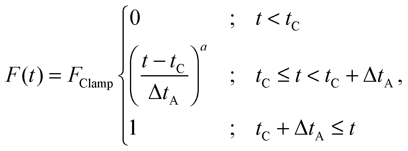
We developed force clamp force mapping (FCFM) as a novel AFM technique. FCFM is based on force mapping (FM), an AFM imaging mode used to determine the local elastic properties of a sample by recording force–distance curves. A detailed description of FM can be found elsewhere.28 In FCFM, the cantilever is vertically approached to the cell at a constant velocity (here: vAppr = 8 μm s−1) (Fig. 1a and b, left). After tip-sample contact at time tC, the apparent force on the cantilever (Fig. 1c, gray trace) increases. The approach is stopped when a pre-defined force FClamp (here: FClamp = 400 pN) is reached. In contrast to FM where the tip would now be retracted from the sample, the force is clamped at the value FClamp by a feedback loop controlling the z-position of the cantilever for a pre-defined force clamp period ΔtClamp (Fig. 1, green area). While the force clamp is active, the viscoelastic creep of the cell leads to an increasing indentation of the cell (Fig. 1d, black trace). We set ΔtClamp = 64 ms, which was a compromise between a high mapping rate and a high fitting accuracy. This timescale lies within the experimentally obtained frequency range that is governed by power-law rheology (about 0.01–100 s).21 Finally, the cantilever is retracted from the cell at a constant velocity (here: vRetr = 35 μm s−1), which was chosen larger than vAppr to speed up the measurement (Fig. 1, right).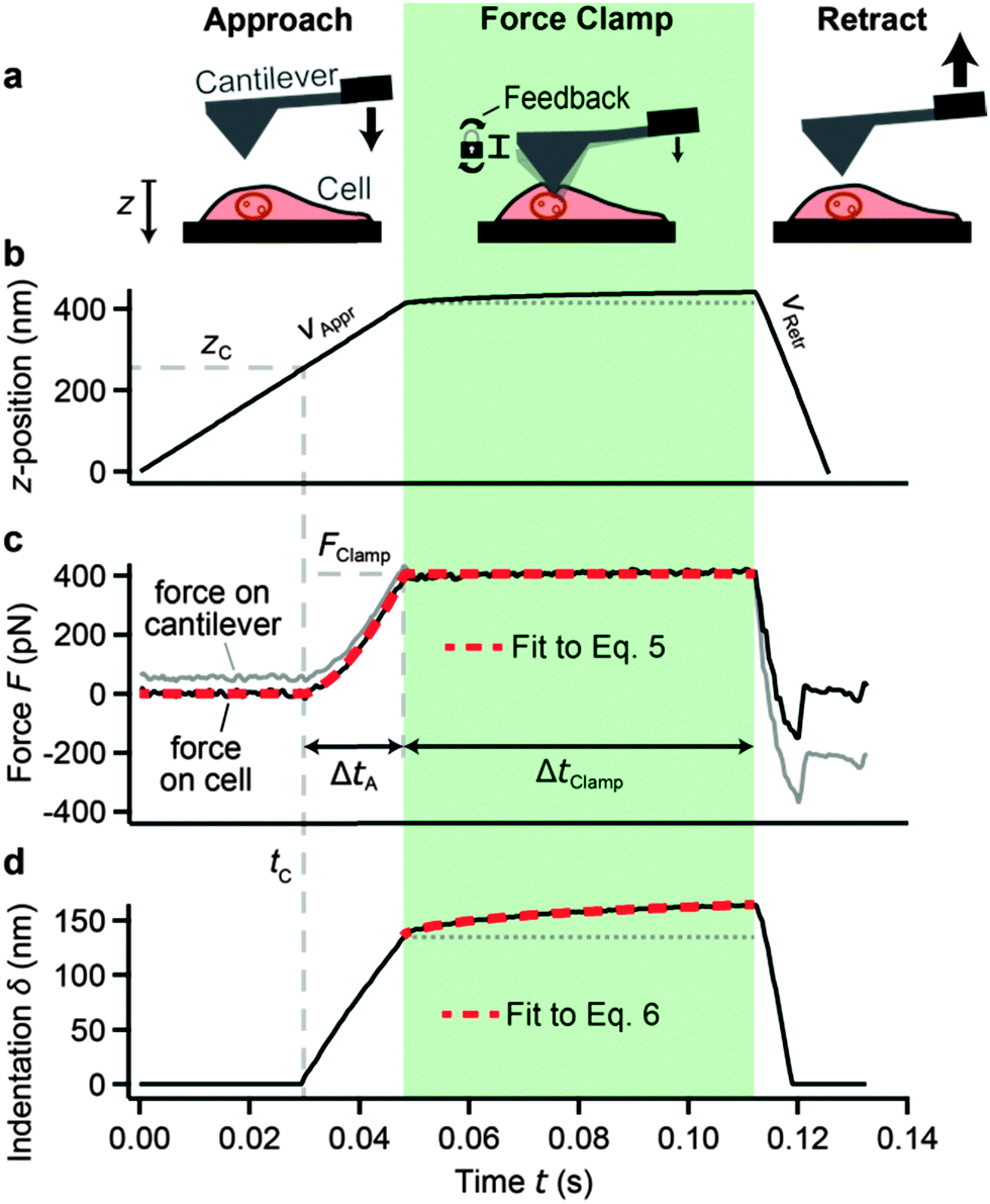 | ||
| Fig. 1 Force clamp force mapping (FCFM). (a) Principle of FCFM. At each xy-position on the cell, force–distance measurements are carried out in three phases: approach (left), force clamp (middle, green area), and retraction (right). (b) z-position of the cantilever base. The approach and retraction velocities (vAppr and vRetr, respectively) are constant. During force clamp, the z-position slightly increases owing to the active z-feedback, which compensates for indentation creep. (c) Force acting on the cantilever (gray trace, includes viscous drag from the surrounding fluid) and force on the cell [black trace, corrected for viscous drag using eqn (1)]. The force on the cantilever starts increasing at the point of contact tC. The approach is stopped when the force reaches the setpoint force FClamp. A force feedback loop maintains this force for a time period ΔtClamp (force clamp). Fitting eqn (5) to the data of the approach and the force clamp phase (red dashed trace) allows for a parameterization of the applied force history. (d) Indentation of the tip into the cell (black trace). Fitting eqn (6) to the indentation creep during the force clamp phase (red dashed trace) gives the modulus scaling parameter E0 and the power-law exponent β (here: E0 = 29.9 ± 0.1 kPa, β = 0.141 ± 0.001). This procedure is repeated for each xy-position on the cell to give two-dimensional maps of E0 and β. | ||
To correct the measurement for the viscous drag by the surrounding fluid on the cantilever, we estimated the viscous drag force from the velocity of the cantilever tip vTip(t) (Fig. S1, ESI†). We then obtained the net force on the cell F(t) from the measured cantilever deflection d(t) by subtracting the viscous drag force
| F(t) = kd(t) − μvTip(t), | (1) |
| δ(t) = [z(t) − zC] − [(d(t) − dC)]. | (2) |
2.2 Theoretical model
The relation between an increasing loading force F(t) on a rigid indenter that is penetrating a linear viscoelastic body and the corresponding indentation depth δ(t) was first derived by Lee and Radok.35 For a pyramidal indenter,36
 | (3) |
The creep compliance of a power-law material is
 | (4) |
 | (5) |
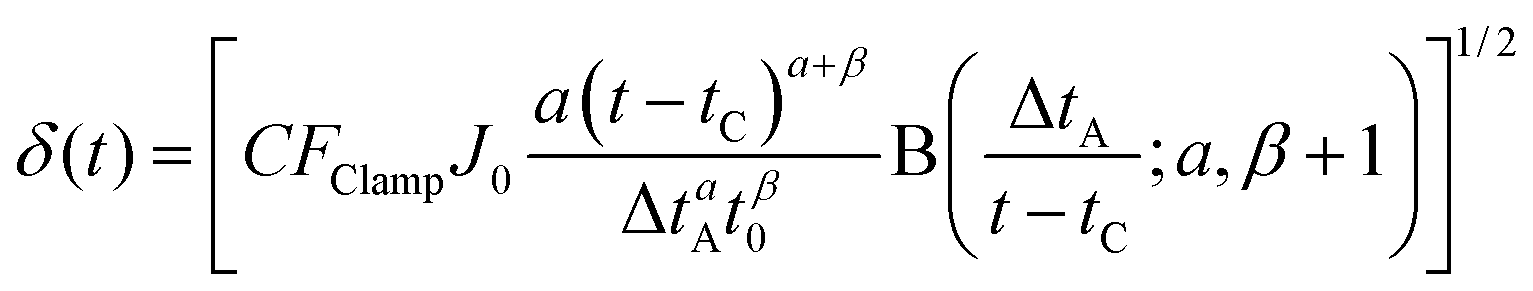 | (6) |
2.3 Validation of FCFM on polyacrylamide gels
We applied FCFM to viscoelastic polyacrylamide (PAA) gels. The contact height map (Fig. 2a) shows the flat gel surface with an RMS (root-mean-square) roughness of 16 nm. The modulus scaling parameter E0 (Fig. 2b) shows a log-normal distribution, ranging from about 4.5 kPa to 6.5 kPa with a mean of E0 = 5.3 kPa (Fig. 2b, histogram). The power-law exponent β (Fig. 2c) shows a normal distribution, ranging from about 0.07 to 0.12 with a mean value of β = 0.091 (Fig. 2c, histogram). The mean values of E0 and β correspond to a storage modulus of E′ = 5 kPa, a loss modulus of E′′ = 0.7 kPa, and a loss tangent of E′′/E′ = 0.14 (see Materials and methods), which is consistent with results from oscillatory AFM measurements40 and from macroscopic rheometer measurements.41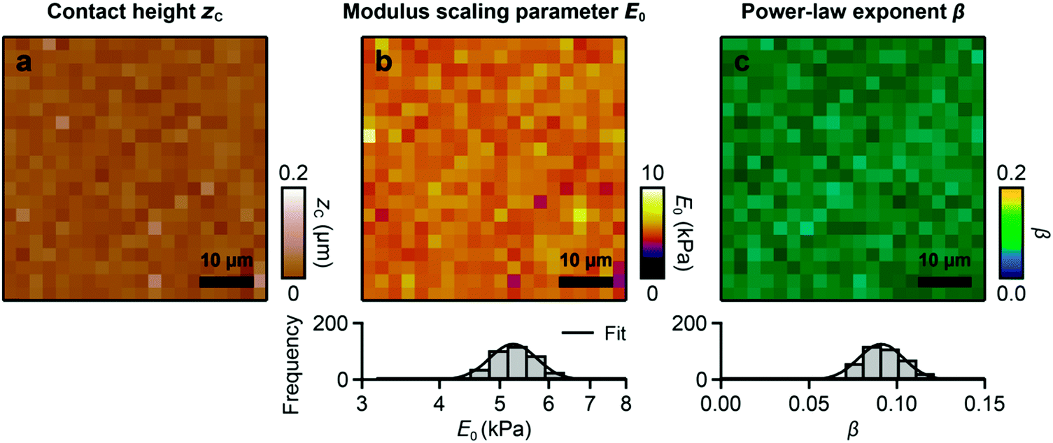 | ||
| Fig. 2 Force clamp force mapping (FCFM) on a polyacrylamide (PAA) gel. (a) Map of contact height zC. (b) Map of the modulus scaling parameter E0, showing a log-normal distribution (histogram). (c) Map of the power-law exponent β, showing a normal distribution (histogram). Pixel resolution is 20 × 20 pixels. | ||
2.4 Spatially resolved maps of the power-law parameters of live cells
FCFM was applied to live MEF cells. Fig. 3 shows one representative dataset. The contact height map (Fig. 3a) shows the undeformed cell topography. The modulus scaling parameter map (Fig. 3b) reveals fibrous structures of elevated E0 (white arrows). A histogram of E0 within the cell shows an approximately log-normal distribution, ranging from 10–100 kPa (Fig. 3b, histogram). The power-law exponent β of the cell shows a systematic spatial variation (Fig. 3c). Elevated values of β are mostly found in the cells’ peripheral regions (black arrows). Histograms of β show an approximately normal distribution, ranging from 0.1–0.2 (Fig. 3c, histogram). A log-normal distribution of the cells’ modulus scaling parameter and a normal distribution of the power-law exponent have previously been reported when many cells were measured at one position each.42,43 Our data show that such distributions also apply to a single cell when measured at multiple positions.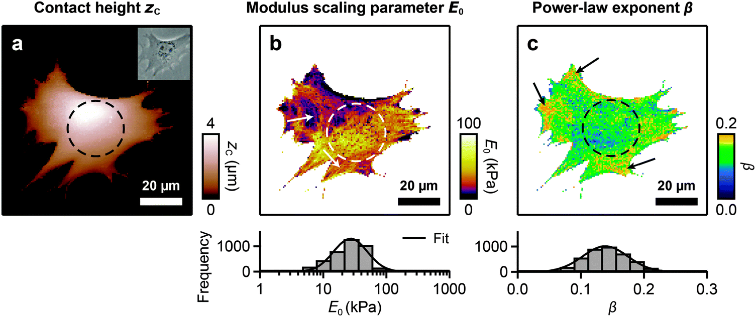 | ||
| Fig. 3 Force clamp force mapping (FCFM) on a live MEF vin−/− cell. (a) Map of contact height zC. An optical phase contrast image (inset) shows the position of the nucleus (marked by dashed circles in the maps). (b) Map of the modulus scaling parameter E0. Stiff fibrous structures can be identified, which are most likely cytoskeletal fibers (white arrows). Within the cell, E0 approximately follows a log-normal distribution ranging from about 10 kPa to 100 kPa (histogram). (c) Map of the power-law exponent β. The peripheral areas exhibit relatively high values of β (black arrows). Within the cell, β approximately follows a normal distribution ranging from about 0.1 to 0.2 (histogram). Pixel resolution is 140 × 140 pixels. All pixels identified as substrate (z < 100 nm) are colored white. | ||
The cell nucleus, which is clearly seen in the optical image (Fig. 3a, inset), cannot be clearly identified in the maps of E0 or β. This suggests that nuclear mechanical properties, if they are different to those of the cytoskeleton, did not significantly affect the E0 or β maps. Furthermore, we evaluated whether the maps are influenced by cell morphology or the underlying substrate. We found that there is no significant correlation between E0 or β and the sample slope (Fig. S2a–c, ESI†). This indicates that measurement artifacts caused by slipping or sticking of the cantilever tip on inclined sample regions, and thus the influence of cell morphology, are negligible. We found a correlation between E0 or β and zC only for cell heights zC < 500 nm (Fig. S2d and e, ESI†), indicating that the influence of the underlying substrate is negligible above a height of 500 nm.
2.5 Vinculin affects the power-law scaling parameters j0 and τ0 of MEF cells
We tested whether FCFM can be used to quantify the effect of a protein knockout on the power-law rheological properties of MEF cells. To test this in a robust manner, we measured maps of 40 MEF WT and 33 MEF vin−/− cells and computed the median of E0 and β for each cell of both cell populations (Fig. 4a and b). E0 and β strongly vary between the cells and approximately range from 5–50 kPa and from 0.05–0.25, respectively. Furthermore, log(E0) and β exhibit a negative linear correlation, in line with previous results.10,21,23,29–32,44 The means values of E0 and β, however, do not differ significantly for WT and vin−/− cells (p > 0.6) (Fig. 4c and d). Interestingly, while the cell-to-cell variation (geometric standard deviation) of E0 does not differ significantly for WT and vin−/− cells (p > 0.3) (Fig. 4e), the cell-to-cell variation (standard deviation) of β is significantly smaller for WT than for vin−/− cells (p < 10−7) (Fig. 4f).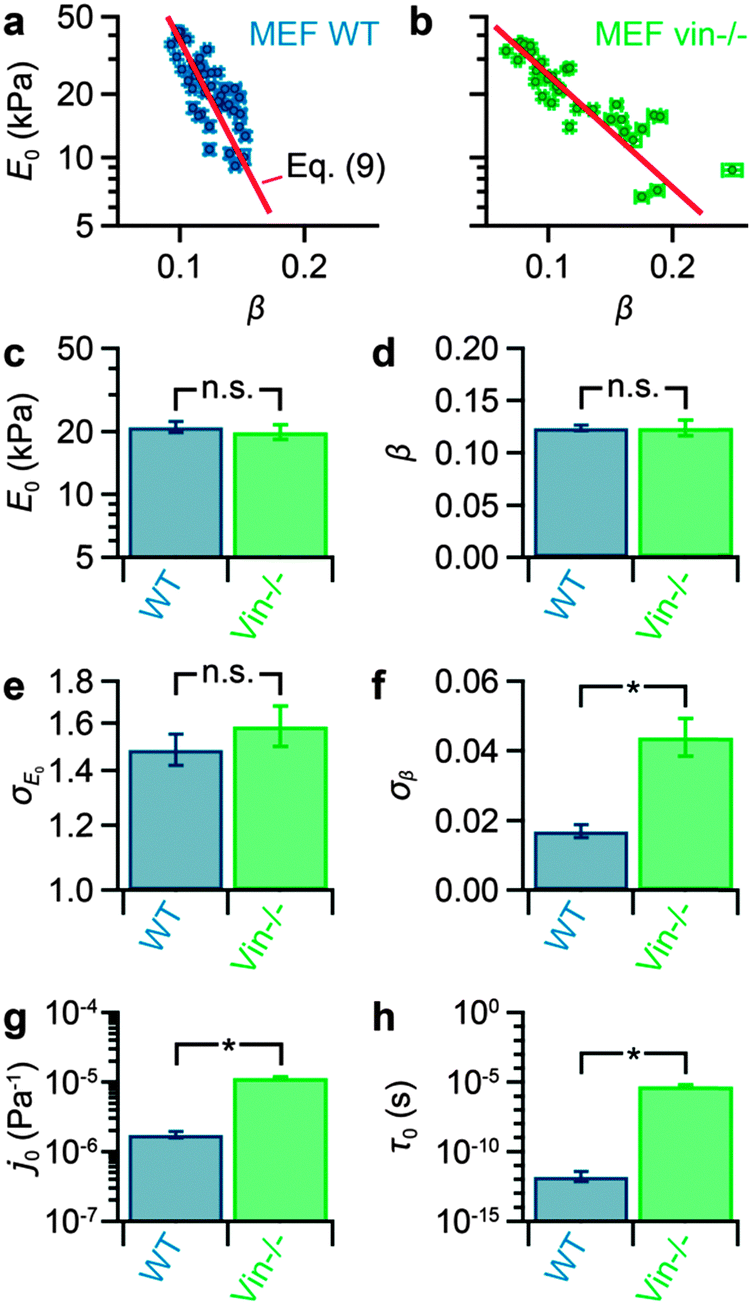 | ||
| Fig. 4 Effect of vinculin knockout on the medians of modulus scaling parameter E0 and power-law exponent β and on the scaling parameters j0 and τ0 in MEF cells. (a) Correlation plots of E0 and β for MEF WT and (b) for MEF vin−/− cells, showing a linear correlation between log(E0) and β. The red curves represent least square fits of eqn (7). (c) The mean modulus scaling parameter E0 shows no significant difference between WT (E0 = 21 ± 1 kPa) and vin−/− (E0 = 20 ± 2 kPa) cells (p = 0.61). (d) The mean power-law exponent β does not exhibit a significant difference between WT (β = 0.124 ± 0.003) and vin−/− (β = 0.124 ± 0.008) cells (p = 0.97). (e) The cell-to-cell variation σE0 of the modulus scaling parameter E0 shows no significant difference between WT (σE0 = 1.48+0.07−0.06) and vin−/− (σE0 = 1.58+0.09−0.09) cells (p = 0.36). (f) However, the cell-to-cell variation σβ of the power-law exponent β significantly differs between WT (σβ = 0.017 ± 0.002) and vin−/− (σβ = 0.044 ± 0.005) cells (p < 10−7). (g) The scaling parameter j0 obtained from the fits in panels a and b shows a significant difference between WT cells (j0 = 1.7+0.2−0.2 × 10⁻⁶ Pa−1) and vin−/− cells (j0 = 1.1+0.3−0.3 × 10⁻⁵ Pa−1) (p < 10−7). (h) The scaling parameter τ0 also indicates a significant difference between WT (τ0 = 1.6+2.2−0.9 × 10⁻¹² s) and vin−/− cells (τ0 = 5.3+1.5−1.2 × 10⁻⁶ s) (p < 10−7). Error bars denote the standard error. Asterisks denote significant differences (p < 0.01) and “n.s.” denotes no significant differences (p > 0.01). | ||
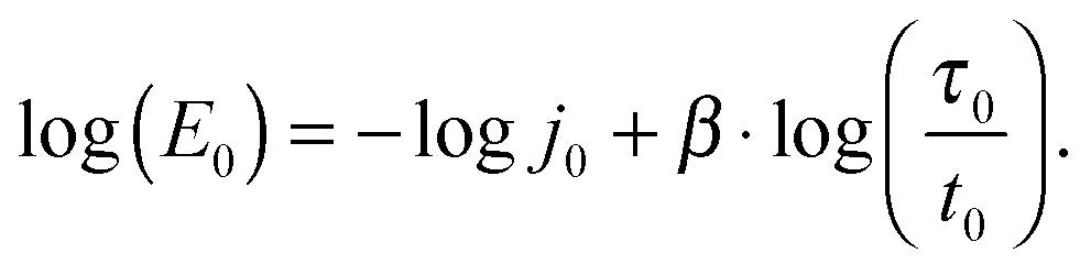
From a linear correlation between log(E0) and β, it follows that there are two more scaling parameters,21 here denoted as j0 and τ0. In this case, eqn (4) rewrites as J(t) ≕ j0(t/τ0)β, giving
 | (7) |
3. Discussion and conclusion
We developed FCFM, a new AFM technique for mapping the viscoelastic properties of single cells with high spatial resolution by including a brief creep behavior measurement into the traditional force-indentation protocol. We validated FCFM on soft polyacrylamide gels and demonstrated that the method provides quantitative viscoelastic sample properties in agreement with other, well-established methods. We found that the creep behavior of cells is well recapitulated by a power-law material model, in agreement with oscillatory AFM measurements.18,19,21,23,45,46 For the first time, we mapped the modulus scaling parameter E0 and the local power-law exponent β over the entire surface of single live MEF cells, with a lateral pixel resolution of about 600 nm and a pixel rate of up to 7 Hz. Mapping was facilitated by a fast measurement protocol with a duration down to 0.14 s at each sample position. This duration is faster compared to previous, oscillatory AFM measurements on living cells, where the measurement at each position required several seconds.19,21,23,45,46 However, oscillatory AFM measurements can provide viscoelastic properties over a wide frequency range without assuming a material model.The local values for E0 range from approximately 10–100 kPa (Fig. 3b) and those for β from approximately 0.1–0.2 (Fig. 3c), which is in good agreement with previously reported data obtained by measuring many cells at one position each.16–22,43,47–49 The distributions of both log(E0) and β are well described by normal distributions, which is also consistent with data obtained by optical magnetic twisting cytometry,50 AFM,23 and optical stretcher48 measurements. The recorded rheological maps indicate that elevated values of β are more likely to be found in peripheral regions of the cell. Although a comprehensive microscopic interpretation of β is still missing, it has been proposed that β represents the turn-over dynamics of cytoskeletal proteins and cross-linkers, including myosin motor activity.10 Cytoskeletal protein dynamics is essential for contraction and locomotion51 and has been reported to be higher in peripheral areas of the cell such as in the lamella and the lamellipodium, resulting in elevated values for β. Cell organelles such as the cell nucleus were not visible in the maps of E0 or β, however.
We measured the medians of E0 and β for each of 40 MEF WT and 33 MEF vin−/− cells to gain a robust data set for further analysis. The medians of E0 and β strongly varied across the measured cells. The population means of E0 and β and the cell-to-cell variation of E0 did not show a significant influence of vinculin knockout. However, the cell-to-cell variation of β differed significantly for WT and vin−/− cells.
As a next step, we used FCFM to determine the scaling parameters j0 and τ0 of both cell populations. In previous studies, j0 and τ0 has been determined by extrapolating creep or frequency responses from cells with different pharmacological treatments29–33 or from cells with different baseline stiffnesses.34 Extrapolation over several orders of magnitude in time or frequency, far beyond the measurement time scale,21,23,30,33 however leads to inaccuracies.29,30,33 Here, we performed the measurement at a fixed time scale and determined the scaling parameters j0 and τ0 by fitting log(E0) vs. β for multiple cells (Fig. 4a and b). The so-determined scaling parameters j0 and τ0 showed large and statistically significant differences between wild-type and knockout cells. Such differences have previously found only between cells of different origin,29–33 but not for cells of the same type that differed only in the expression levels of a protein.
Power-law rheology and collapse of log(E0) vs. β onto a master curve is predicted by the theory of soft glassy materials, which derives power-law rheological properties from weak binding interactions of disordered, non-thermally agitated structural elements in a complex energy landscape. Accordingly, τ0 is the minimum time interval between reorganization processes, and j0 is the compliance of the material at the glass transition where reorganization processes no longer occur.9 Applied to cells, 1/τ0 can be interpreted as the maximum frequency beyond which the cytoskeleton exhibits no reorganization dynamics and reaches its maximum “rigor” stiffness of 1/j0.21 Following this interpretation, j0 and τ0 can also be understood as cell-type-specific parameters that define the range of power-law rheological behavior that is “allowed” to the cell.10 Consequently, a cell cannot “vary” its stiffness independently from β, but only along a specific master curve, which is represented by the red curves in Fig. 4a and b.
It appears that the knockout of vinculin as part of the focal adhesion complex52 decreases the maximum or “rigor” stiffness 1/j0 and slows down the molecular reorganization dynamics of the cytoskeleton. Vinculin is an important protein for coupling mechanical forces from the cytoskeleton to the extracellular matrix.53,54 Loss of vinculin leads to a decrease of cytoskeletal tension,55–57 which is linearly related to the stiffness of adherent cells.34,58 This is consistent with our finding that the stiffness of vin−/− cells is decreased compared to WT cells. When measuring the creep behavior at physiologically relevant and experimentally attainable sub-second or second time scales, however, the differences between WT and vin−/− cells can become obscured. But these differences can be uncovered by the parameters j0 and τ0 that scale the elastic and dissipative cell properties onto master curves. Here, we provided evidence that the scaling parameters j0 and τ0 are not only cell-type-specific constants,21,29–32 but that they are significantly influenced by the knockout of a single protein. Thus, FCFM is a powerful AFM mode for characterizing viscoelastic sample properties.
4. Materials and methods
4.1 Power-law rheology
The viscoelastic behavior of live cells can be described by a power-law over several decades in time or frequency (from about 0.01–100 s or 0.01–100 Hz, respectively).22,59 In this range, the time-dependent creep compliance J(t), which is the ratio of strain ε(t) to mechanical stress in response to a force step, can be described as J(t) = J0(t/t0)β. Analogously, the frequency-dependent complex modulus G(f) also follows a power-law: G(f) ∼ fβ. The power-law exponent β is a dimensionless number that characterizes the degree of dissipation or “fluidity”33 of such a power-law material, where β = 0 corresponds to a purely elastic solid and β = 1 to a purely viscous Newtonian fluid. The power-law exponent of live cells typically covers a relatively wide range from about 0.1–0.5, as was observed with different measurement techniques.16,18,23,34,43 The power-law pre-factor J0 = J(t = t0) is a measure of the material's compliance at the time t = t0. J0 and t0 cannot be determined independently of each other in a single measurement, owing to the scaling invariance. Hence, the time scaling parameter t0 can be chosen arbitrarily and is usually set to t0 = 1 s. We define the scaling parameter for the material's modulus as E0 = 1/J0, which can therefore be understood as the apparent Young's modulus of the material at a timescale of 1 s.We also used the conventional, purely elastic Hertzian contact model adapted for pyramidal tips37 to extract an apparent Young's modulus E from the approach part of the force–distance curves. For the PAA gel we found that the mean value of E (5.4 kPa, Fig. S3a, ESI†) was slightly larger than the previously obtained mean value of E0 (5.3 kPa, Fig. 2b); for the cell we found that the mean value of E (43 kPa, Fig. S3b, ESI†) was larger than the previously obtained mean value of E0 (26 kPa, Fig. 3b). This is because E depends on the time scale of the indentation,60 which is shorter than the chosen time scaling parameter t0 = 1 s of the E0-values obtained with FCFM.
From the parameters E0 and β the complex modulus E* = E′ + iE′′ of the material can be estimated using the storage modulus E′ ≅ E0Γ(β + 1)cos(βπ/2) and the loss modulus E′′ ≅ E0Γ(β + 1)sin(βπ/2), which are related by the loss tangent tan![[thin space (1/6-em)]](https://www.rsc.org/images/entities/char_2009.gif) θ ≅ E′′/E′ = tan(βπ/2).29Gamma denotes the gamma function.
θ ≅ E′′/E′ = tan(βπ/2).29Gamma denotes the gamma function.
While the time scaling parameter t0 can be chosen arbitrarily, it was found that for live cells there exists an invariant time scale τ0, where the compliance values J0 for different cells of a given cell type merge to a single value j0.21 Interestingly, the power-law creep compliance of cells under different pharmacological treatments seems to “pivot” around the point given by (j0,τ0).29–33 The existence of this pivoting point implies that E0 and β are not independent but must change together along a master curve. The parameters j0 and τ0 that scale E0 and β onto a master curve thus contain additional information about the cells’ mechanical properties. Importantly, j0 and τ0 were found to depend on the cell type10 and thus can be used to detect differences between cell types even when cell rheology measurements overlap.
4.2 Cell culture
The cells used in this study were mouse embryonic fibroblast wild-type cells (MEF WT, 40 cells) and mouse embryonic fibroblast vinculin knockout cells (MEF vin−/−, 33 cells).55,57 Both cell populations were cultured in DMEM (Life Technologies, Paisley, UK) supplemented with 10% (v/v) heat inactivated fetal bovine serum and 1% (v/v) L-glutamine with penicillin-streptomycin (PAA Laboratories, Pasching, Austria) and were kept at 37 °C with 5% CO2. One day before measurements, the cells were seeded in 50 mm fibronectin-coated (50 μg ml−1, Roche Applied Science, Basel, Switzerland) culture dishes (Greiner Bio-One, Kremsmünster, Austria) at a density of 500 cells per cm2. About 1 h before an experiment, the medium was replaced with CO2 independent Leibovitz L-15 medium (Life Technologies, Paisley, UK). The cells were measured at 37 °C. Two separate preparations were measured for each cell population.4.3 Polyacrylamide gel preparation
Glass coverslips were incubated in 2% 3-aminopropyltrimethoxysilane solution (Sigma-Aldrich, Taufkirchen, Germany). The coverslips were then incubated in 1% glutaraldehyde solution (Sigma-Aldrich, Taufkirchen, Germany). Afterwards, a drop of acrylamide/bis-acrylamide (w/w 29:1) solution (Sigma-Aldrich, Taufkirchen, Germany) in deionized water with a final acrylamide concentration of 4.8% was pipetted onto each coverslip. Gel polymerization was initiated by adding ammonium persulfate (APS) (Sigma-Aldrich, Taufkirchen, Germany) and N,N,N′,N′-tetramethylethylenediamine (TEMED) (Sigma-Aldrich, Taufkirchen, Germany) to the solution. The apparent mean Young's modulus of the gel of E = 5.4 kPa (Fig. S3a, ESI†) is in good agreement with a previously measured Young's modulus of about 6 kPa for a similar preparation as used here.61Fig. 2 and Fig. S4 (ESI†) show two representative datasets out of a total of four FCFM measurements on PAA gels.
4.4 AFM
The measurements were carried out using an atomic force microscope (MFP-3D-BIO, Asylum Research, Santa Barbara, CA) combined with an inverted phase contrast light microscope (Ti-S, Nikon, Tokio, Japan) to monitor the cells during the mapping process. Cantilevers with pyramidal tips (MLCT-C, Bruker, Camarillo, CA) with a nominal semi-included angle (axis-to-face) of α = 19.2° and a nominal spring constant of 0.01 N m−1 were used. Before each measurement, the spring constant was calibrated in air using the thermal noise method.62 The deflection and z-position data were recorded at a sampling rate of 2 kHz. The apparent force on the cantilever was calculated from the deflection by multiplication with the spring constant (Hooke's law). To demonstrate that FCFM also works for other tip shapes, the measurements on the PAA gel were repeated with different cantilevers. Measurements with symmetric square pyramidal tips (DNP, Veeco, Santa Barbara, CA) with a nominal semi-included angle (axis-to-face) of α = 35° and a nominal spring constant of 0.06 N m−1 gave similar results (Fig. S4, ESI†).In single cell (Fig. 1, 3 and Fig. S5, ESI†) and PAA gel (Fig. 2 and Fig. S4, ESI†) measurements, FClamp was set to 400 pN, ΔtClamp to 64 ms, and vAppr to 6–8 μm s−1 (unless stated otherwise). To speed up the measurements, cells were pre-scanned with a low pixel resolution (25 × 25 pixel). Mapping with a high pixel resolution was conducted only within the cell contours, with a pixel resolution of 640–950 nm, which took approximately 20–50 min. The contact height images were flattened line-by-line to generate the height data shown as topography images. Pixels with a contact height smaller than 100 nm were defined as substrate pixels and colored white in the maps of E0 and β. Optical phase contrast images were acquired prior to the start of the mapping process (Fig. 3a, inset). In measurements on multiple cells (Fig. 4), the mapping resolution was reduced to 50 × 50 pixels to increase the measurement throughput. In these experiments, FClamp was set to 600 pN, ΔtClamp to 48 ms, and vAppr to 3 μm s−1. We found that the resulting values of E0 and β do not depend considerably on the selected experimental parameters FClamp, ΔtClamp, and vAppr (see Fig. S5, ESI†).
Application of multiple, closely-spaced creep response measurements in rapid succession did not alter the viscoelastic properties of the sample e.g. due to mechano-chemical signal transduction, since no stripe artifacts between trace and retrace were observed in the maps. Thin regions of the cell (zc < 500 nm) showed a significant correlation between modulus scaling parameter and contact height (see Fig. S2d and e, ESI†) and were therefore excluded from analysis to reduce artifacts due to the underlying substrate.
4.5 Data analysis
For the modulus scaling parameter E0 and the scaling parameters j0 and τ0, the log-transformed values were used for median calculation, averaging, statistical tests, and fitting, because these parameters closely follow a log-normal distribution.29,30 The error bars in Fig. 4a and b denote the standard error estimated from the standard deviation σ using the consistent estimator σ = 1.4826 × MAD,63 where MAD denotes the median absolute deviation, which is defined as the median of the absolute deviations from the data's median. The fits to E0 and β were weighted by these standard errors to provide reliable error estimates for the fit parameters. Data processing and analysis were carried out with IGOR Pro 6 (Wavemetrics, Portland, OR). All reported p-values were calculated with the two-tailed, unpaired Student's t-test or F-test; statistical significance was assumed at p < 0.01.Acknowledgements
We thank Christoph Braunsmann, Vera Auernheimer, and Jan Seifert for discussions and assistance in cell culture. This work was supported by grants from the Ministry for Science, Research and Art Baden-Württemberg, Bayerische Forschungsallianz, Deutscher Akademischer Austauschdienst, and Deutsche Forschungsgemeinschaft (FA336/7-1). We thank Asylum Research for technical support.References
- E. M. Reichl, J. C. Effler and D. N. Robinson, Trends Cell Biol., 2005, 15, 200–206 CrossRef CAS PubMed.
- S. Kumar and V. M. Weaver, Cancer Metastasis Rev., 2009, 28, 113–127 CrossRef PubMed.
- S. Huang and D. E. Ingber, Nat. Cell Biol., 1999, 1, E131–E138 CrossRef CAS PubMed.
- M. E. Chicurel, C. S. Chen and D. E. Ingber, Curr. Opin. Cell Biol., 1998, 10, 232–239 CrossRef CAS.
- P. A. Janmey, Physiol. Rev., 1998, 78, 763–781 CAS.
- J. T. Parsons, A. R. Horwitz and M. A. Schwartz, Nat. Rev. Mol. Cell Biol., 2010, 11, 633–643 CrossRef CAS PubMed.
- G. Bao and S. Suresh, Nat. Mater., 2003, 2, 715–725 CrossRef CAS PubMed.
- H. Huang, R. D. Kamm and R. T. Lee, Am. J. Physiol.: Cell Physiol., 2004, 287, C1–C11 CrossRef CAS PubMed.
- P. Sollich, Phys. Rev. E: Stat. Phys., Plasmas, Fluids, Relat. Interdiscip. Top., 1998, 58, 738–759 CrossRef CAS.
- P. Kollmannsberger and B. Fabry, Annu. Rev. Mater. Res., 2011, 41, 75–97 CrossRef CAS.
- E. A. Evans, Biophys. J., 1983, 43, 27–30 CrossRef CAS.
- A. R. Bausch, F. Ziemann, A. A. Boulbitch, K. Jacobson and E. Sackmann, Biophys. J., 1998, 75, 2038–2049 CrossRef CAS.
- Y. Tseng, T. P. Kole and D. Wirtz, Biophys. J., 2002, 83, 3162–3176 CrossRef CAS.
- J. Guck, R. Ananthakrishnan, H. Mahmood, T. J. Moon, C. C. Cunningham and J. Käs, Biophys. J., 2001, 81, 767–784 CrossRef CAS.
- G. Binnig, C. F. Quate and C. Gerber, Phys. Rev. Lett., 1986, 56, 930–933 CrossRef.
- J. M. Maloney, D. Nikova, F. Lautenschläger, E. Clarke, R. Langer, J. Guck and K. J. Van Vliet, Biophys. J., 2010, 99, 2479–2487 CrossRef CAS PubMed.
- G. Massiera, K. M. Van Citters, P. L. Biancaniello and J. C. Crocker, Biophys. J., 2007, 93, 3703–3713 CrossRef CAS PubMed.
- S. Hiratsuka, Y. Mizutani, A. Toda, N. Fukushima, K. Kawahara, H. Tokumoto and T. Okajima, Jpn. J. Appl. Phys., 2009, 48, 08JB17 CrossRef.
- J. Alcaraz, L. Buscemi, M. Grabulosa, X. Trepat, B. Fabry, R. Farré and D. Navajas, Biophys. J., 2003, 84, 2071–2079 CrossRef CAS.
- S. Nawaz, P. Sánchez, K. Bodensiek, S. Li, M. Simons and I. A. T. Schaap, PLoS One, 2012, 7, e45297 CAS.
- B. Fabry, G. N. Maksym, J. P. Butler, M. Glogauer, D. Navajas and J. J. Fredberg, Phys. Rev. Lett., 2001, 87, 148102 CrossRef CAS.
- B. D. Hoffman, G. Massiera, K. M. Van Citters and J. C. Crocker, Proc. Natl. Acad. Sci. U. S. A., 2006, 103, 10259–10264 CrossRef CAS PubMed.
- P. Cai, Y. Mizutani, M. Tsuchiya, J. M. Maloney, B. Fabry, K. J. Van Vliet and T. Okajima, Biophys. J., 2013, 105, 1093–1102 CrossRef CAS PubMed.
- M. Radmacher, R. W. Tillmann and H. E. Gaub, Biophys. J., 1993, 64, 735–742 CrossRef CAS.
- H. Haga, M. Nagayama, K. Kawabata, E. Ito, T. Ushiki and T. Sambongi, J. Electron Microsc., 2000, 49, 473–481 CrossRef CAS.
- S. Moreno-Flores, R. Benitez, M. d. Vivanco and J. L. Toca-Herrera, J. Biomech., 2010, 43, 349–354 CrossRef PubMed.
- A. Raman, S. Trigueros, A. Cartagena, A. P. Z. Stevenson, M. Susilo, E. Nauman and S. Antoranz Contera, Nat. Nanotechnol., 2011, 6, 809–814 CrossRef CAS PubMed.
- M. Radmacher, J. P. Cleveland, M. Fritz, H. G. Hansma and P. K. Hansma, Biophys. J., 1994, 66, 2159–2165 CrossRef CAS.
- B. Fabry, G. N. Maksym, J. P. Butler, M. Glogauer, D. Navajas, N. A. Taback, E. J. Millet and J. J. Fredberg, Phys. Rev. E: Stat., Nonlinear, Soft Matter Phys., 2003, 68, 041914 CrossRef.
- G. Lenormand, E. Millet, B. Fabry, J. P. Butler and J. J. Fredberg, J. R. Soc. Interface, 2004, 1, 91–97 CrossRef CAS PubMed.
- R. E. Laudadio, E. J. Millet, B. Fabry, S. S. An, J. P. Butler and J. J. Fredberg, Am. J. Physiol.: Cell Physiol., 2005, 289, C1388–C1395 CrossRef CAS PubMed.
- B. A. Smith, B. Tolloczko, J. G. Martin and P. Grütter, Biophys. J., 2005, 88, 2994–3007 CrossRef CAS PubMed.
- J. M. Maloney and K. J. Van Vliet, Soft Matter, 2014, 10, 8031–8042 RSC.
- P. Kollmannsberger, C. T. Mierke and B. Fabry, Soft Matter, 2011, 7, 3127–3132 RSC.
- E. H. Lee and J. R. M. Radok, J. Appl. Mech., 1960, 27, 438–444 CrossRef.
- M. Sakai, Philos. Mag. A, 2002, 82, 1841–1849 CAS.
- G. G. Bilodeau, J. Appl. Mech., 1992, 59, 519–523 CrossRef.
- M. Radmacher, M. Fritz, C. M. Kacher, J. P. Cleveland and P. K. Hansma, Biophys. J., 1996, 70, 556–567 CrossRef CAS.
- C. Braunsmann, R. Proksch, I. Revenko and T. E. Schäffer, Polymer, 2014, 55, 219–225 CrossRef CAS PubMed.
- R. E. Mahaffy, C. K. Shih, F. C. MacKintosh and J. Käs, Phys. Rev. Lett., 2000, 85, 880–883 CrossRef CAS.
- C. A. Grattoni, H. H. Al-Sharji, C. Yang, A. H. Muggeridge and R. W. Zimmerman, J. Colloid Interface Sci., 2001, 240, 601–607 CrossRef CAS PubMed.
- N. Desprat, A. Richert, J. Simeon and A. Asnacios, Biophys. J., 2005, 88, 2224–2233 CrossRef CAS PubMed.
- M. Balland, N. Desprat, D. Icard, S. Féréol, A. Asnacios, J. Browaeys, S. Hénon and F. Gallet, Phys. Rev. E: Stat., Nonlinear, Soft Matter Phys., 2006, 74, 021911 CrossRef.
- S. Yamada, D. Wirtz and S. C. Kuo, Biophys. J., 2000, 78, 1736–1747 CrossRef CAS.
- J. Rother, H. Nöding, I. Mey and A. Janshoff, Open Biol., 2014, 4, 140046 CrossRef PubMed.
- L. M. Rebêlo, J. S. de Sousa, J. M. Filho, J. Schape, H. Doschke and M. Radmacher, Soft Matter, 2014, 10, 2141–2149 RSC.
- R. Sunyer, X. Trepat, J. J. Fredberg, R. Farré and D. Navajas, Phys. Biol., 2009, 6, 025009 CrossRef CAS PubMed.
- J. M. Maloney, E. Lehnhardt, A. F. Long and K. J. Van Vliet, Biophys. J., 2013, 105, 1767–1777 CrossRef CAS PubMed.
- C. J. Chan, G. Whyte, L. Boyde, G. Salbreux and J. Guck, Interface Focus, 2014, 4, 20130069 CrossRef CAS PubMed.
- C. Y. Park, D. Tambe, A. M. Alencar, X. Trepat, E. H. Zhou, E. Millet, J. P. Butler and J. J. Fredberg, Am. J. Physiol.: Cell Physiol., 2010, 298, C1245–C1252 CrossRef CAS PubMed.
- D. A. Lauffenburger and A. F. Horwitz, Cell, 1996, 84, 359–369 CrossRef CAS.
- P. Kanchanawong, G. Shtengel, A. M. Pasapera, E. B. Ramko, M. W. Davidson, H. F. Hess and C. M. Waterman, Nature, 2010, 468, 580–584 CrossRef CAS PubMed.
- R. M. Ezzell, W. H. Goldmann, N. Wang, N. Parasharama and D. E. Ingber, Exp. Cell Res., 1997, 231, 14–26 CrossRef CAS PubMed.
- I. Thievessen, P. M. Thompson, S. Berlemont, K. M. Plevock, S. V. Plotnikov, A. Zemljic-Harpf, R. S. Ross, M. W. Davidson, G. Danuser, S. L. Campbell and C. M. Waterman, J. Cell Biol., 2013, 202, 163–177 CrossRef CAS PubMed.
- C. T. Mierke, P. Kollmannsberger, D. P. Zitterbart, J. Smith, B. Fabry and W. H. Goldmann, Biophys. J., 2008, 94, 661–670 CrossRef CAS PubMed.
- C. Möhl, N. Kirchgeßner, C. Schäfer, K. Küpper, S. Born, G. Diez, W. H. Goldmann, R. Merkel and B. Hoffmann, Cell Motil. Cytoskeleton, 2009, 66, 350–364 CrossRef PubMed.
- C. T. Mierke, P. Kollmannsberger, D. P. Zitterbart, G. Diez, T. M. Koch, S. Marg, W. H. Ziegler, W. H. Goldmann and B. Fabry, J. Biol. Chem., 2010, 285, 13121–13130 CrossRef CAS PubMed.
- N. Wang, K. Naruse, D. Stamenović, J. J. Fredberg, S. M. Mijailovich, I. M. Tolić-Nørrelykke, T. Polte, R. Mannix and D. E. Ingber, Proc. Natl. Acad. Sci. U. S. A., 2001, 98, 7765–7770 CrossRef CAS PubMed.
- L. Deng, X. Trepat, J. P. Butler, E. J. Millet, K. G. Morgan, D. A. Weitz and J. J. Fredberg, Nat. Mater., 2006, 5, 636–640 CrossRef CAS PubMed.
- C. Braunsmann, J. Seifert, J. Rheinlaender and T. E. Schäffer, Rev. Sci. Instrum., 2014, 85, 073703 Search PubMed.
- A. Engler, L. Bacakova, C. Newman, A. Hategan, M. Griffin and D. Discher, Biophys. J., 2004, 86, 617–628 CrossRef CAS.
- S. M. Cook, T. E. Schäffer, K. M. Chynoweth, M. Wigton, R. W. Simmonds and K. M. Lang, Nanotechnology, 2006, 17, 2135–2145 CrossRef CAS.
- D. C. Hoaglin, F. Mosteller and J. W. Tukey, Understanding robust and exploratory data analysis, Wiley, New York, 1983 Search PubMed.
Footnotes |
| † Electronic supplementary information (ESI) available. See DOI: 10.1039/c4sm02718c |
| ‡ Both authors contributed equally to this publication. |
| This journal is © The Royal Society of Chemistry 2015 |