DOI:
10.1039/C4SM02477J
(Paper)
Soft Matter, 2015,
11, 2193-2202
Electrohydrodynamic patterning of ultra-thin ionic liquid films
Received
8th November 2014
, Accepted 19th January 2015
First published on 20th January 2015
Abstract
In the electrohydrodynamic (EHD) patterning process, electrostatic destabilization of the air–polymer interface results in micro- and nano-size patterns in the form of raised formations called pillars. The polymer film in this process is typically assumed to behave like a perfect dielectric (PD) or leaky dielectric (LD). In this study, an electrostatic model is developed for the patterning of an ionic liquid (IL) polymer film. The IL model has a finite diffuse electric layer which overcomes the shortcoming of assuming infinitesimally large and small electric diffuse layers inherent in the PD and LD models respectively. The process of pattern formation is then numerically simulated by solving the weakly nonlinear thin film equation using finite difference with pseudo-staggered discretization and an adaptive time step. Initially, the pillar formation process in IL films is observed to be the same as that in PD films. Pillars initially form at random locations and their cross-section increases with time as the contact line expands on the top electrode. After the initial growth, for the same applied voltage and initial film thickness, the number of pillars on IL films is found to be significantly higher than that in PD films. The total number of pillars formed in 1 μm2 area of the domain in an IL film is almost 5 times more than that in a similar PD film for the conditions simulated. In addition, the pillar structure size in IL films is observed to be more sensitive to initial film thickness compared to PD films.
1. Introduction
Numerous studies have been conducted on the electrohydrodynamic (EHD) process since initial exploration1 of this technique where a conical shape is formed on a sessile drop after placing a charged rod close to the top.2–6 Early studies focused on either perfect conductor (PC) liquids like water and mercury or perfect dielectrics (PD) like benzene. Deformation and the bursting of fluid drops in the presence of an electric field are experimentally examined,4 resulting in understanding the role of conductivity in behavior of an isolated emulsion drop in an electric field.3 This resulted in the theory of leaky dielectric (LD) or poorly conducting materials. EHD flow is being intensively studied due to extensive industrial applications such as de-emulsification,7 microfluidics,8 lab on a chip9,10 and soft lithography.11–14
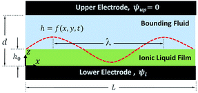
In electrohydrodynamic lithography (EHL), a molten thin polymer film which is heated to above its glass transition temperature is subjected to an electric field to destabilize the film to create well-controlled micro- and nano-patterns. The film patterning process relies on the EHD flow in the polymer film; so this process will be modeled and simulated. The EHD patterning process starts with an initially flat (thermal motion is neglected) liquid thin film that is confined between two electrodes (the thin film is denoted as h0 in Fig. 1). The liquid film is bounded with either air or another polymer film to fill the gap between electrodes. Applying a transverse electric field induces the electric pressure (Maxwell stress) at the film interface that perturbs the pressure balance and enhances the most unstable wavelength of growing instabilities on the film interface. Various structures form on the polymer surface depending on the initial filling ratio (ratio of initial film thickness to electrode distance) of the polymer film,15 the electric permittivity ratio of layers (film and bounding media),16,17 the shape of the electrodes16,17 and the surface energy of the electrodes and the polymer film.18,19
 |
| | Fig. 1 Schematic view of the thin film sandwiched between electrodes. h = f(x, y, t) is the film height described by the function with the lateral coordinates and time. λ is the maximum growing wavelength. | |
The majority of experimental and theoretical studies are performed considering the liquid thin film layers to be either perfect dielectrics (PD),11,13,15,19 with no free charge, or leaky dielectrics (LD),12,14,20,21 with an infinitesimal amount of charges. In ideal PD materials the conductivity is zero; so when a potential difference is applied across the PD material, the electric field and potential drop depend on the electric permittivity. In LD materials, charges move and accumulate on the interface when an electric field is applied. When the charge relaxation time (the time required for movement of charges in response to electric field) is larger than the growth rate of instabilities, LD films can be modeled by the PD theory. When charges migrate and accumulate at the interface before the pattern formation occurs, then the charge conservation equation must be solved simultaneously with the fluid flow equations. The presence of free charges at the interface results in a significant decrease in the film structure length scale.21
In this study the liquid thin film is assumed to be an ionic liquid. An IL is defined as a salt like material liquid below 100 °C or electrolyte (aqueous or nonaqueous). Free ions present in the ILs and in contact with charged surfaces move toward the oppositely charged surfaces and form a diffuse layer, called the double layer (DL). The DL is characterized by its thickness and Debye length.22 This diffuse layer, associated with the equilibrium charge, is absent in EHD patterning of PCs, PDs and LDs.11,12,15,20,21,23
How a complete electrokinetic model seamlessly bridges the gap between perfect dielectric and leaky dielectric models was summarized by Zholkovskij et al.24 How the EK model accounts for double layer confinement and overlap in a liquid cell has also been addressed.25 To study electrically induced interfacial instabilities of ionic (conducting) fluid films using stability analysis, an electrokinetic model was recently presented.26 These authors used an analytical solution of the linearized Debye Hückel electrokinetic model to assess the ionic layer stability. For low conductivity fluids, the Debye length was found to have a considerable effect on the wavelength of the instabilities when the ionic fluid layer thickness is comparable to the Debye length. In the previous cases of ionic liquid films,26,27 the linearized Poisson equation (the Debye Hückel model) was used for the electrostatic governing equation. In analyses utilizing the Debye Hückel model, care must be taken not to apply too high an electric potential. Furthermore, electric break down of the polymer film in high electric fields has an intrinsic limitation in nano-scale EHD patterning processes.27,28 A more detailed numerical study from our group29 solved the complete Poisson–Nernst–Planck equation for the ionic layer, and came to the conclusion that a full EK model provides a better understanding of the EHD patterning in ionic fluids compared to leaky dielectric models.
The dynamics of ions are modeled by ion conservation.30 Conductivity of an IL depends on the molar concentration of ions and a higher concentration results in higher conductivity of electrolytes.26 Electrolytes with high molar concentration have a thinner diffuse layer or Debye length. However, the dynamics of charges in a LD material and ions in ILs can be neglected when the process time is much larger than the charge relaxation time and such a system is in quasi-equilibrium.20
To the best of authors' knowledge, dynamics, instability and the process of pattern formation of IL films under an applied electric field for the EHD patterning process has not been studied. In this work, a system consisting of two planar fluid layers (thin IL film below and PD bounding media above) confined between two flat electrodes is considered. When a transverse electric field is applied in the IL film the free ions move and accumulate close to the charged surfaces (lower electrode and film interface) and form a diffuse layer.
An electrostatic model is developed for an IL film in contact with a PD bounding media to obtain the electric potential distribution and consequently the net electrostatic pressure acting on the interface. The electrostatic pressure model is then used in the nonlinear thin film equation to investigate the dynamics, instability and process of pattern formation in the EHD patterning process. The size and shape of formed structures are compared with previous results for PD films11,15,19 of different thicknesses. The contributions of this paper are: (1) developing an electrostatic model for dynamic modeling of the EHD patterning process using ultra-thin IL films; (2) investigating the dynamics and pattern formation on IL films. This includes the initial linear stages and further nonlinear stages in growth of instabilities; and (3) evaluating the effects of ionic strength and the IL film initial thickness on the shape and size of structures that form on the film.
2. Problem formulation
A thin film system consisting of two layers where the fluid layers are assumed to be Newtonian and incompressible with a constant viscosity, μ, density, ρ and electric permittivity ε is shown in Fig. 1. Unless otherwise indicated, constants and parameters used in the model are listed in Table 1.
Table 1 Constants or parameters used in modeling
| Parameter |
Value |
| Interfacial tension (γ) |
0.048 N m−1 |
| Viscosity of liquid film (μ) |
1 Pa s |
| Effective Hamaker constant (A) |
−1.5 × 10⁻²¹ J |
| Permittivity of vacuum (ε0) |
8.85 × 10⁻¹² C V−1 m−1 |
| Electric permittivity of the liquid film (ε1) |
2.5 (−) |
| Electric permittivity of the bounding media (ε2) |
1 (−) |
| Molarity (M) |
0.00001–0.01 mol L−1 |
| Initial film thickness (h0) |
20–70 nm |
| Electrodes distance (d) |
100 nm |
| Equilibrium distance (l0) |
1–7 nm |
| Applied voltage (ψl) |
20 V |
2.1 Hydrodynamics
The dynamics and evolution of thin polymer films are described by mass and momentum conservation. For a single layer EHD patterning process, the liquid film is usually bounded with air. Air can be considered as an inert gas since its viscosity is much less than that of the liquid film. The liquid layer is thin enough so that gravity effects are negligible. Effects due to inertia are also neglected due to a very small Reynolds number.20,26 With these assumptions the simplified governing mass and momentum equations of the film are:| | ∇·![[u with combining right harpoon above (vector)]](https://www.rsc.org/images/entities/i_char_0075_20d1.gif) 1 = 0 1 = 0 | (1) |
| | −∇P1 + μ∇21 + ![[f with combining right harpoon above (vector)]](https://www.rsc.org/images/entities/i_char_0066_20d1.gif) e = 0 e = 0 | (2) |
Boundary conditions are:
(i) No slip condition on the electrodes, z = 0 and z = d
| i = 0 |
(ii) No penetration (two media are immiscible):
| relative = 0 |
| (iii) Stress balance at the interface, z = h(x, y, t) |
(iv) Kinematic boundary conditions at the interface,31z = h(x, y, t)
where
![[small sigma, Greek, macron]](https://www.rsc.org/images/entities/i_char_e0d2.gif)
= −
PĪ +
μi(∇
i + (∇
i)
T). The subscript
i denotes the fluid phase (here 1 for the thin polymer film and 2 for air) and subscripts
t,
x and
y stand for derivatives with respect to time,
x and
y directions, respectively.
κ* is the mean surface curvature,
γ is surface tension, and
![[n with combining right harpoon above (vector)]](https://www.rsc.org/images/entities/i_char_006e_20d1.gif)
and
![[t with combining right harpoon above (vector)]](https://www.rsc.org/images/entities/i_char_0074_20d1.gif) i
i are the normal and tangent vectors of the interface, respectively.
32
The external body force, e = −∇ϕ (eqn (2)), accounts for the contribution of external forces to the fluid flow. The term ϕ is the conjoining pressure and it is a summation of intermolecular forces (van der Waals and Born repulsive) and electrostatic forces.15
In eqn (3) the term ϕvdW is used for the van der Waals forces, defined as ϕvdW = Al/6πh3 for the lower electrode. The lower electrode is assumed to have higher energy compared to the polymer film; therefore the polymer film is initially stable. Under these conditions the coefficient Al is negative33 which induces the repulsive van der Waals force. The term ϕBr is the Born repulsive force, defined as ϕBr = 8BU/(d − h)9 for the upper electrode. The Born repulsive force is a short range force and is used to avoid nonphysical penetration of a liquid into the solid phase, mainly for the case in which the interface touches the upper electrode. The coefficient BU is found by setting the conjoining pressure, ϕ, equal to zero at h = d − l0 to maintain a maximum equilibrium film thickness (l0 is the equilibrium distance). The last term in eqn (3), ϕE, is the electrostatic component of the conjoining pressure which is obtained from Maxwell stress34 and a more detailed derivation follows.
Applying an electric field results in the perturbations of the air–polymer interface, h(x, y, t). Initial perturbations grow most quickly with the fastest growing instability wavelength of λ, which is much larger than the initial film thickness, h0; so a “long-wave approximation”35 can be used to simplify the equations. Using these assumptions results in the “thin film” equation19,36 that describes the spatiotemporal evolution of a film interface as:
| | | 3μht + [h3(γ[hxx + hyy] − ϕ)x]x + [h3(γ[hxx + hyy] − ϕ)y]y = 0 | (4) |
The term 3μht is for viscous force present in the system.13 The term γ[hxx + hyy] is the surface tension force which damps fluctuations33 and minimizes the interface area of the film and the ϕ term is given in eqn (3).
2.2 Electrostatic pressure
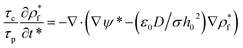
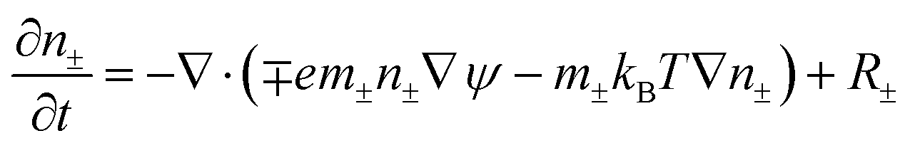
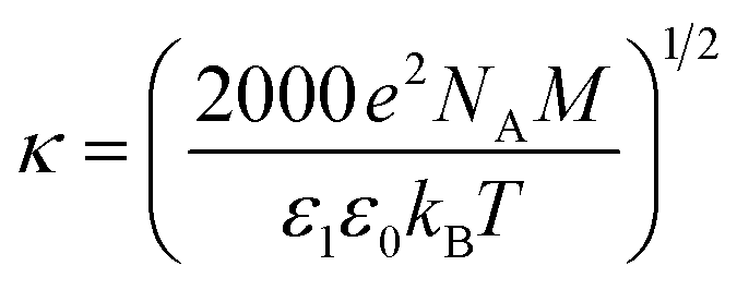
To solve the thin film dynamics it is necessary to have an electrostatic model for ϕE for PD–PD and PD–IL systems. The derivation of the PD–PD systems is well known and reproduced here for completeness. Throughout this study, it is assumed that electric breakdown does not occur during the EHD patterning process. Using electrolytes, a particular case of ILs, free ions have the ability to migrate or redistribute within the liquid and accumulate on the charged surfaces forming a DL. More details about DL and its regions are presented in the literature.22,37 The ion conservation equation for the dynamics of free ions in the electrolytes, based on the number concentration of the free monovalent ions (n+ and n−), is:| |  | (5) |
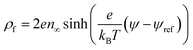
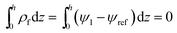
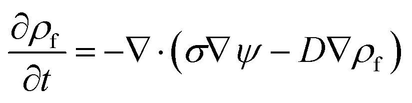
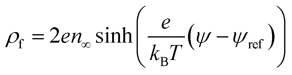
The left hand side of this equation represents the accumulation rate. The first term on the right hand side is the net flux due to migration and diffusion, respectively. Ion migration is induced by the electric potential gradient, ∇ψ, and the diffusion is the result of concentration gradient ∇n±. The last term, R±, is the production rate of species due to chemical reactions which is set to zero in this study. m± is the mobility and e is the elementary charge. The Boltzmann constant kB = 1.3806488 × 10⁻²³ (m2 kg s−2 K−1) and T (°K) is temperature. Using definitions for free charge density ρf = e(n+ − n−), conductivity σ = e(m+n+ + m−n−) and mobility m = D/kBT (D is diffusion coefficient), the ion conservation equation is:
| |  | (6) |
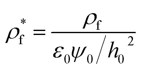
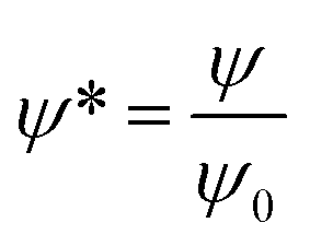
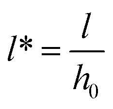
This equation is then scaled using nondimensional terms ( ,
,  ,
,  and
and  ) resulting in:
| |  | (7) |
where,
τp =
μh0/
ε0ε1ψ02 is the process time and
τc =
ε0ε1/
σ is the charge relaxation time.
20 In this study based on the parameters used for simulations,
τp and
τc vary between 2.35–5.85 (s) and 8.92 × 10
−11 to 1.05 × 10
−7 (s), respectively. When the process time is much larger than the charge relaxation time (
τp ≫
τc), the dynamics of free ions (charges) becomes insignificant
14,26 and left-hand sides of
eqn (6) and
(7) become zero. In that case the ion conservation equation (
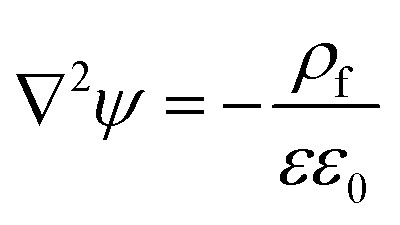
eqn (6)) can be simplified to the Poisson equation.
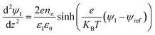
30| |  | (8) |
where,
| |  | (9) |
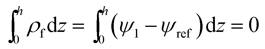
and
n∞ and
ψref are bulk ion number concentration and reference potential, respectively. When the bounding media is air or any PD media,
ρf = 0,
eqn (8) reduces to the Laplace equation. Bulk ion number concentration depends on the molarity of the electrolyte which is defined as
n∞ = 1000
NAM where
M is the electrolyte molar concentration (mol L
−1) and
NA = 6.022 × 10
23 mol
−1 is the Avogadro number. In
eqn (9) the term
kBT represents thermal motion while the term
e(
ψ −
ψref) is the electrostatic contribution caused by the deviation from the electroneutrality condition (
ψref), respectively. The electrostatics governing equations in the long-wave limit
35 for a bounding layer is
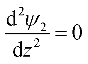
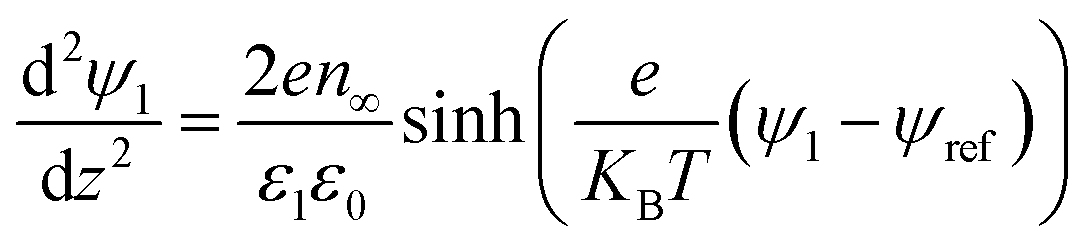
| |  | (10) |
and for an IL film are
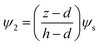
| |  | (11a) |
| |  | (11b) |
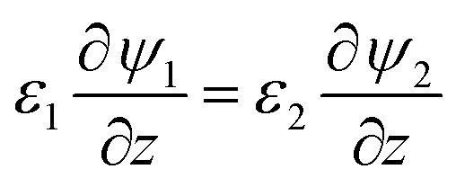
The boundary conditions for eqn (10), (11a) and (11b) are the applied potential on the lower electrode (ψ1 = ψl), grounded upper electrode (ψ2 = 0) and the electric potential and displacement continuity (ψ1 = ψ2 and 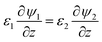 ) at the interface. Eqn (11b) represents conservation of ions within the IL film and is used to find the reference potential, ψref. In this study the Debye Hückel approximation26,30 is used to linearize the Poisson equation transforming eqn (11a) and (11b) to:
| |  | (12a) |
| |  | (12b) |
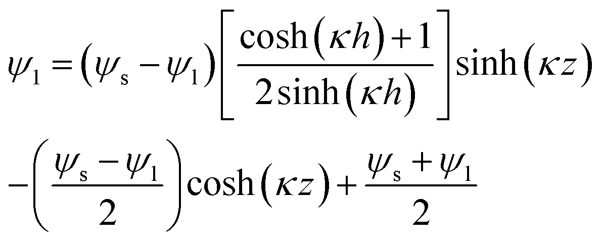
where

is the inverse of Debye length. Solving
eqn (10),
(12a) and
(12b) results in the electric potential distribution within PD and IL layers as follows:
| |  | (13) |
| |  | (14) |
where,
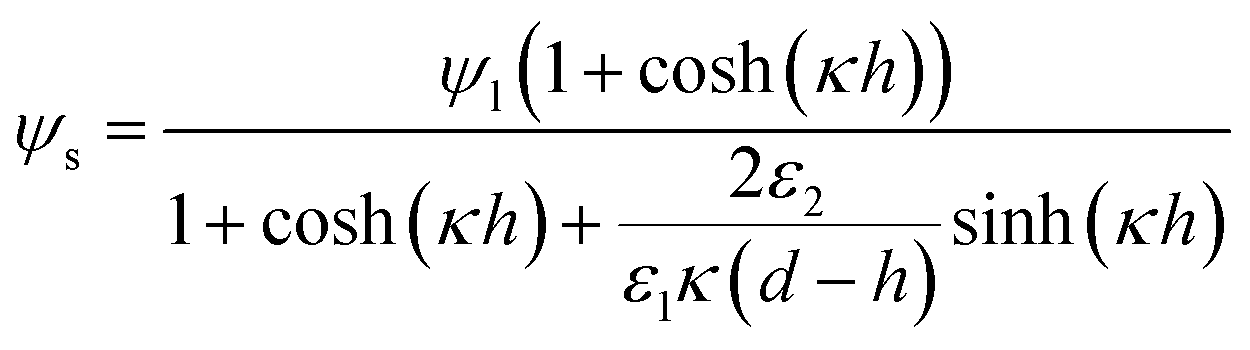
ψs is the interface potential and is determined by the following equation:
| |  | (15) |
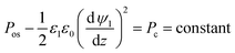
In ionic liquids, an additional force exists between charged surfaces (film interface and lower electrode) due to overlapping of DLs, called the osmotic force and defined as Fos = −dPos/dz.30,38 The osmotic pressure, Pos, has a hydrostatic origin and can be found from the momentum balance in the transverse direction (z). At equilibrium, and assuming that the radius of curvature of the interface is small compared with the IL film thickness (κ*h ≪ 1), this force is balanced with electrostatic force, FE = −ρ(z)(dψ/dz), which results in:39
| |  | (16) |
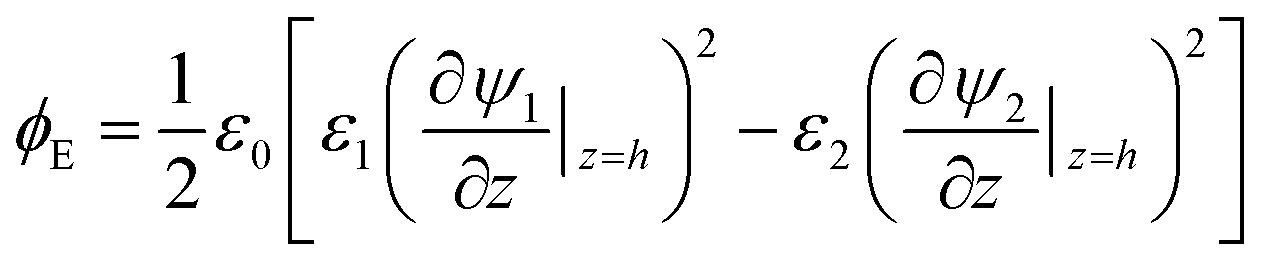
Thus at a given IL film thickness there is always a constant difference between osmotic pressure and electrostatic pressure in eqn (16). The term Pc can be found from a stress balance at the film interface.26 Finally, the term ϕE in eqn (3), which is the net electrostatic pressure in a PD–IL system is given by34
| |  | (17) |
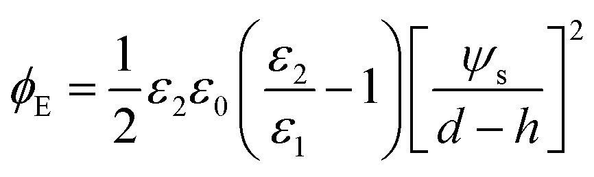
Substituting ψ1 and ψ2 from eqn (13) and (14) into eqn (17) and then using the relationship for ψs in eqn (15) result in the following electrostatic pressure for a PD–IL system,
| |  | (18) |
Finally, the developed electrostatic pressure (eqn (18)) along with van der Waals, ϕvdW, and Born repulsion, ϕBr, pressures are substituted into the thin film equation (eqn (4)) to find the dynamics and spatiotemporal evolution of a thin IL film subjected to a transverse electric field.
2.3 Linear stability analysis
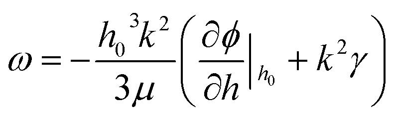
Linear stability (LS) analysis is conducted for a thin IL film (eqn (4)) bounded with a PD bounding layer to predict the characteristic wavelength for growth of instabilities. In LS analysis, the interface height, h, in eqn (4) is disturbed with a small sinusoidal perturbation of the interface, h = h0 + δ![[thin space (1/6-em)]](https://www.rsc.org/images/entities/char_2009.gif) exp(ik(x + y) + ωt). This perturbation has a wavenumber of k, an amplitude of δ and a growth coefficient of ω. The resulting nonlinear terms are neglected and the linear dispersion relationship for the fastest growing wave is found as:
exp(ik(x + y) + ωt). This perturbation has a wavenumber of k, an amplitude of δ and a growth coefficient of ω. The resulting nonlinear terms are neglected and the linear dispersion relationship for the fastest growing wave is found as:| | 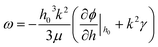 | (19) |
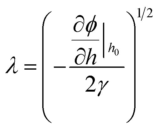
and the resulting maximum growing wavelength is:| |  | (20) |
2.4 Numerical modeling
Various numerical techniques are used to track free interfaces in general,40,41 and in the EHD patterning process specifically.12,15,42,43 These techniques are applied as versatile tools to visualize the transient evolution of a thin liquid film subject to a transverse electric field. In this study, the thin film equations, eqn (4) and (3), are solved numerically to obtain the transient behavior and observe the pattern formation process. The finite difference is used to discretize the spatial derivatives in the 4th order nonlinear partial differential equation (PDE), eqn (4). The resulting differential algebraic equation (DAE) in time is solved by an adaptive time step ordinary differential equation (ODE) solver.44 A square domain with the length of 4λ and periodic boundary conditions are chosen. Initial conditions are set to a small, with an amplitude of 0.005 × h0, random disturbance of the film interface while maintaining liquid film volume constant. The spatial grid size of 121 × 121 is found to be sufficient and used throughout this study.
3. Results and discussion
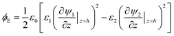
The novelty of this work is the addition of the ionic strength of an IL which is determined by IL molarity, M. This is in addition to typical design parameters such as applied voltage ψl, electric permittivity of layers ε and electrode distance d. Hence, a new parameter the ionic strength of IL, which is determined by IL molarity, M, is added. Higher values of M (= 0.1 and 0.01 mol L−1) account for higher concentration of ions in the layer which results in perfect conducting (PC) behavior whereas lower values of M (= 0.01 and 0.000001 mol L−1) represent a poorly conductive medium similar to PDs.26 The effect of molarity on the electrostatic component of conjoining pressure, as the main force, for the pattern formation process is examined.
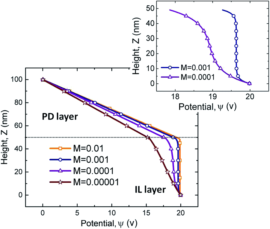
To show the effects of molarity on the electric potential distribution across the film thickness, a 50 nm thick IL film bounded with a 50 nm PD media (e.g. air) is considered. Results for four different values of molarity, M, are presented in Fig. 2. Electric potential distribution from the solution of the Laplace equation in the bounding media (top 50 nm) is linear as expected. For M = 0.01 mol L−1, electric potential reduction across the IL film is almost zero and the IL film behaves like a PC. In this case, the electric field within the IL film is zero. For the limiting case of small molarities, M = 0.00001 mol L−1, the electric potential distribution is similar to that of a PD film. For IL films with molarities between these two limiting values, M = 0.001 and 0.0001 mol L−1, formation of a DL is evident close to the PD–IL interface and lower electrode (see magnified results in Fig. 2). For M = 0.0001 mol L−1, overlapping DL from the interface and the base affects the electroneutrality condition of the entire IL layer. This is due to the large DL thickness, κ−1, as compared to the film thickness. Electroneutrality of the bulk is one main assumption in PD and LD models in the literature11–15,19–21 but does not apply in this case.
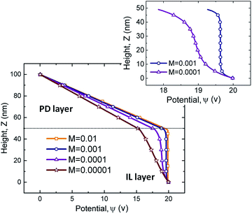 |
| | Fig. 2 Electric potential distribution versus height for four molarity values of M = 0.01, 0.001, 0.0001, and 0.00001 mol L−1 and corresponding Debye lengths, (κ)−1 are: 0.5, 1.7, 5.4 and 17 nm. | |
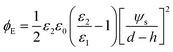
3.1 Electrostatic interaction
The value of interface potential, ψs, a component of the electrostatic conjoining pressure, depends on the molarity of the IL film as well as the electric permittivity ratio of layers, ε1/ε2, and the film thickness, h. Interface potential versus interface height for four molarity values of M = 0.01, 0.001, 0.0001, and 0.00001 mol L−1 are compared in Fig. 3 for a fixed applied potential, ψl, electric permittivity of layers, ε1 and ε2, and electrode distance, d. A lower interface height, h, results in a higher interface potential for all molarities which results in a higher conjoining pressure on the interface (see eqn (18)). For the case in which the PD bounding layer thickness is comparable with the IL film thickness (h = 50 nm in Fig. 3), a higher slope for interface potential occurs for ILs with low molarity indicating that a small change in interface height changes the surface potential considerably. Fig. 3 confirms that at a constant interface height, the rate of potential drop becomes more significant for lower molarities. On the other hand, as the molarity increases, interface potential becomes more insensitive to the interface height which is similar to the behavior of PC films. In the present work ILs are considered as materials whose height–potential relationship lies between the limits of M = 0.01 and 0.00001 mol L−1.
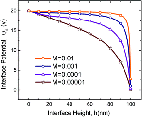 |
| | Fig. 3 Interface potential distributions versus interface height for four molarity values of M = 0.01, 0.001, 0.0001, and 0.00001 mol L−1. ϕl = 20 V, ε1 = 2.5 and ε2 = 1. | |
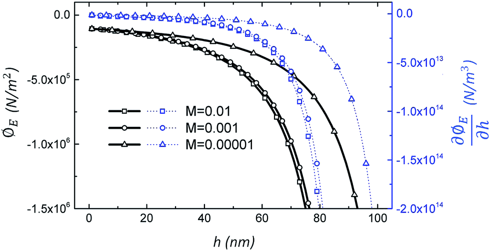
The external force in eqn (2) (defined as a gradient of potential, −∇ϕ) also includes the force due to variation of potential with respect to local film thickness,  . This gradient is called the spinodal parameter and film instability due to this force is called spinodal instability.15 At a given location, when
  , a fluid flows from regions with lower thickness to higher thickness (negative diffusion) leading to growth of instabilities. To investigate the instability of an IL film subjected to an electric field, the term ϕ in eqn (3) is simplified to include only ϕE as the electrostatic component since this is dominant compared to other interactions for the EHD patterning.15 The variations of electrostatic conjoining pressure and the spinodal parameter with interface height for IL films of different molarities are shown in Fig. 4. A negative value of ϕE shows that the electrostatic force pushes the interface toward the upper electrode, often called disjoining force. By increasing the film thickness the electrostatic force is also increased for all three molarity values. Films with higher ion concentration, M = 0.01 and 0.001 mol L−1, experience higher electrostatic forces compared to the low concentration case of M = 0.00001 mol L−1. This difference is more apparent at higher film thicknesses (h0 > 50 nm), i.e. thicker films experience a higher force (more negative) than the thinner ones. This force accelerates growth of instabilities at initial stages to enhance the growth rate of structures at later stages.
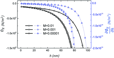 |
| | Fig. 4 Electrostatic pressure, left axis, and spinodal parameter, right axis, distributions versus film thickness for three molarity values of M = 0.01, 0.001 and 0.00001 mol L−1. ϕl = 20 V, ε1 = 2.5 and ε2 = 1. | |
3.2 Scaling results
For thin film time evolution simulation, LS analysis is used to scale length X = x/Ls and Y = y/Ls, time T = t/Ts and conjoining pressure Φ = ϕ/Φs, where| | | Ls = (γε22h03/0.5ε0ε1(ε1 − ε2)ψl2)1/2 | (21a) |
| | | Ts = 3μγε22h03/[0.5ε0ε1(ε1 − ε2)ψl2] | (21b) |
| | | Φs = 0.5ε0ε1(ε1 − ε2)ψl2/(ε22h02) | (21c) |
The interface height is scaled with mean initial film thickness, H = h/h0.
3.3 Perfect dielectric films – baseline
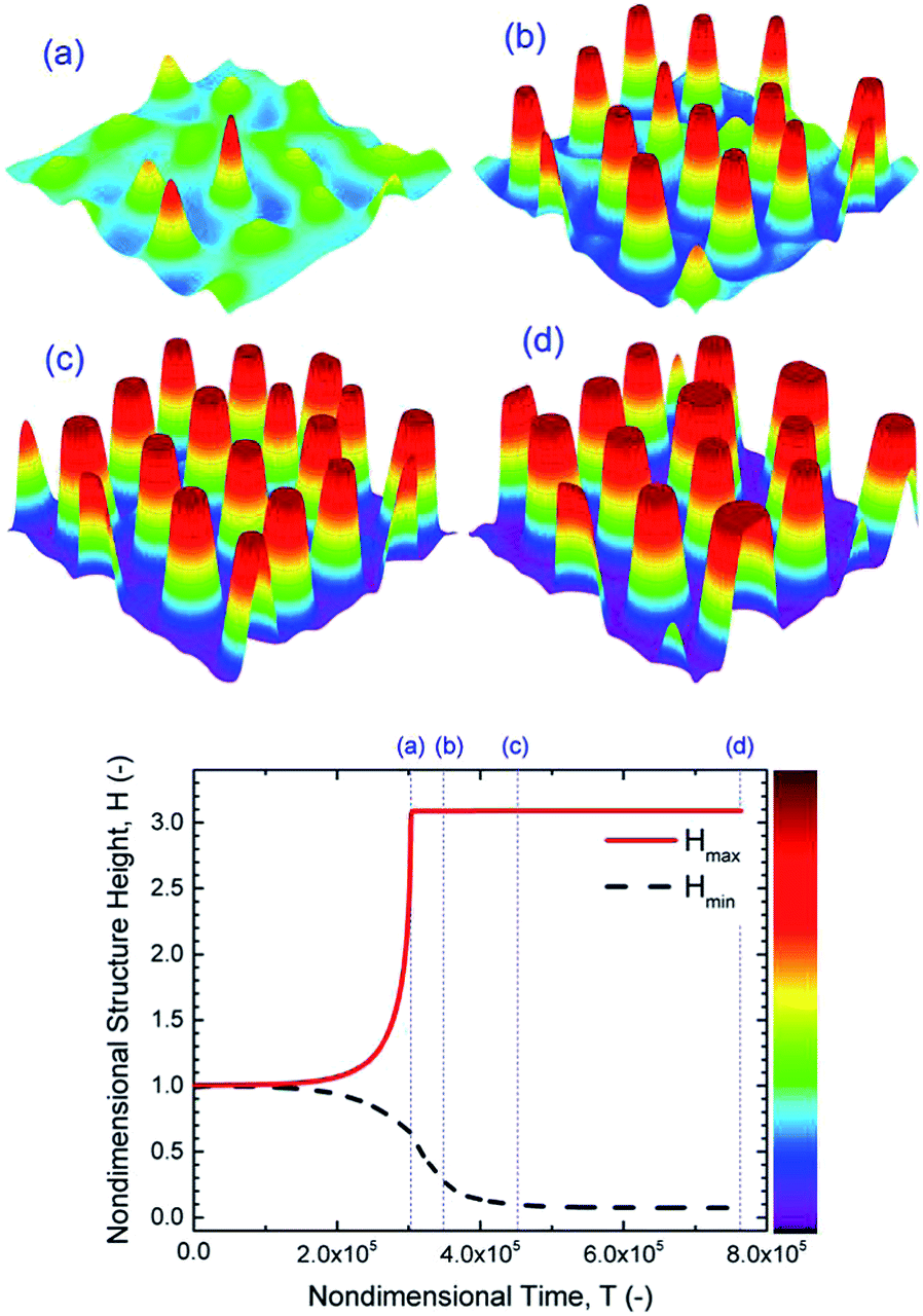
To provide insight into the growth of instabilities in the EHD pattern formation process, PD films with no free ions (ρf = 0) are simulated as a baseline for comparison to IL simulations. Since PD simulation has been done15,19 the accuracy and capability of the numerical method can be checked. First the dynamics and spatiotemporal evolution of the liquid film in response to the transverse electric field are investigated. Nondimensional structure height variations over time and 3-D snapshots of a PD film interface, with an initial film thickness of h0 = 30 nm, are presented in Fig. 5. Tracking the structure height over time shows that the initial random perturbations first grow and when the interface touches the upper electrode for the first time, the minimum height decreases until the film thickness becomes zero. The 3-D snapshots of the PD film interface for four stages of the pattern formation process are shown in Fig. 5(a–d). Fig. 5(a) indicates initial random perturbations and formation of bicontinuous structures. At this stage, ridge fragmentation occurs and isolated islands are formed. The fluid flows from regions with lower thickness to higher thickness and eventually pillars are formed. Pillars initially have a cone shape (Fig. 5(a)) but become more columnar over time (Fig. 5(b)). The pillar height and width increase over time until they reach the upper electrode (Fig. 5(b)). Then as the contact line expands, the pillars grow in cross-section (Fig. 5(c and d)). The results in Fig. 5 match known results15,19 and provide a validation for the code.
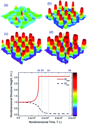 |
| | Fig. 5 PD film with h0 = 30 nm, 3-D spatiotemporal evolution of a PD liquid film (images a–d) and nondimensional structure height variations versus nondimensional time. Nondimensional times, T, are: (a) 3 × 10⁵, (b) 3.5 × 10⁵, (c) 4.5 × 10⁵ and (d) 7.6 × 10⁵, and ψl = 20 V. | |
3.4 Ionic liquid films
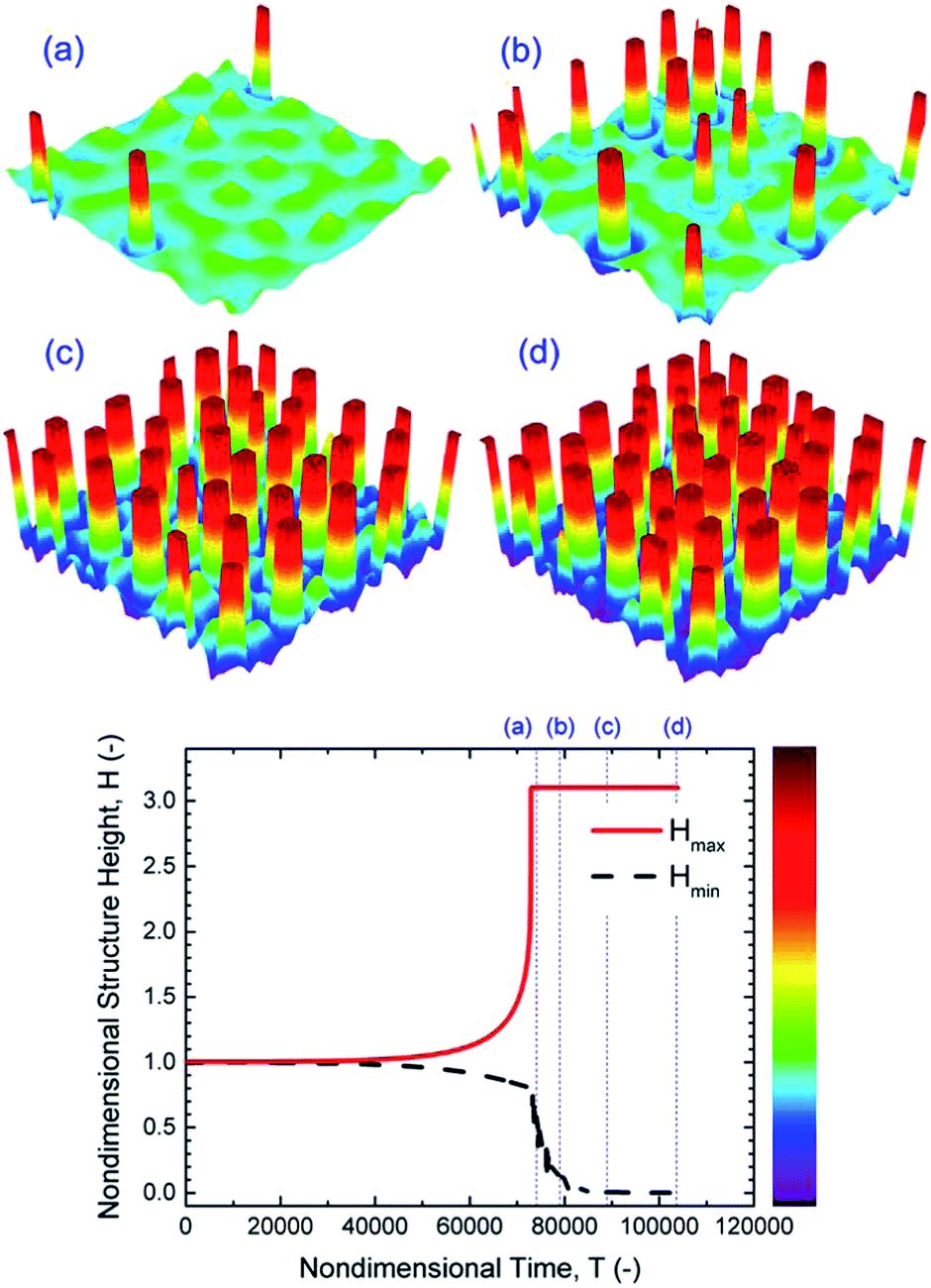
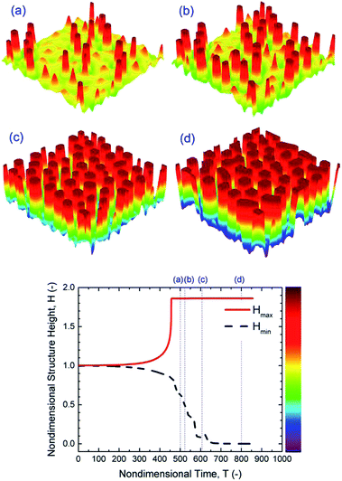
Addition of free ions to the liquid film is found to increase the electrostatic force significantly (Fig. 4). EHD patterning of IL films is investigated in this section. Thin film height and resulting structures as a function of time using 3-D snapshots of an IL film interface, with M = 0.001 mol L−1 and initial film thickness of h0 = 30 nm, are shown in Fig. 6. Tracking of structure height indicates that the first pillar forms after a relatively long time (stage (a)) compared to the total time required for termination of the pillar formation process (stages (a–d)) and compared to PD films (Fig. 5). The same sequence of pillar formation in IL films compared to PD films is observed; however, the pillars in IL films have a smaller cross-section than those in PD films (Fig. 5 and 6). For the IL film, pillars are initially formed on the random locations and enlarged in cross-section with time as the contact line expands on the top electrode. The growth of pillars after touching the upper electrode depletes the liquid around pillars and forms ring-like depressions around them which are apparent in stage (b).
 |
| | Fig. 6 IL film with h0 = 30 nm, 3-D spatiotemporal evolution of an IL film (images a–d) and nondimensional height variations versus nondimensional time. Nondimensional times, T, are: (a) 7.4 × 10⁴, (b) 7.9 × 10⁴, (c) 8.9 × 10⁴ and (d) 1 × 10⁵. M = 0.0001 mol L−1 and ψl = 20 V. | |
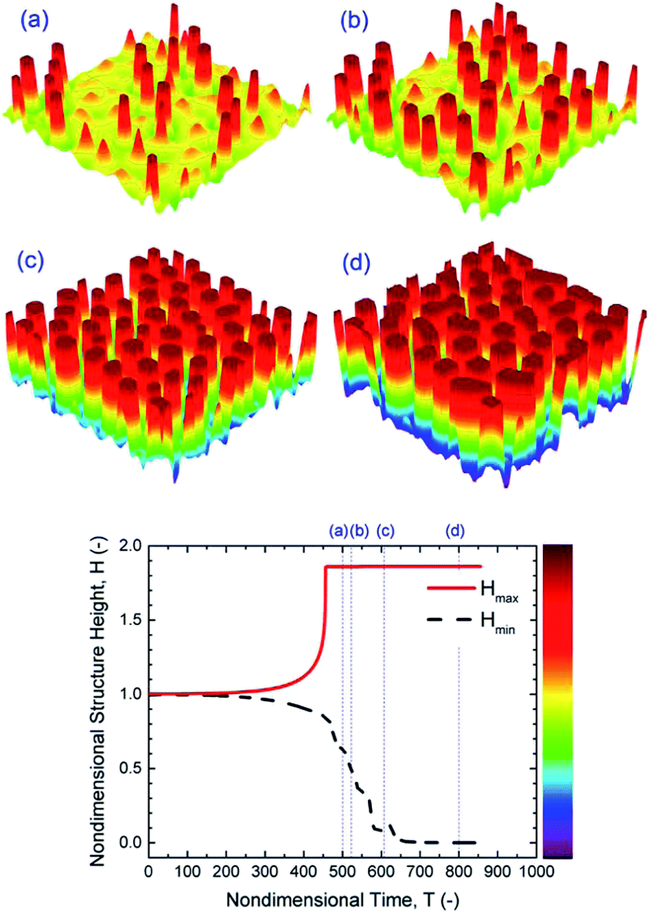
Increasing the initial film thickness of an IL film from h0 = 30 to 50 nm results in faster growth of instabilities and ultimately a faster pattern formation process (Fig. 7). However, these patterns are less stable since neighboring pillars tend to coalesce at later stages (Fig. 7(d)). Faster pattern formation and coalescence of pillars at higher initial film thicknesses are also observed in PD films.
 |
| | Fig. 7 IL film with h0 = 50 nm, 3-D spatiotemporal evolution of a IL liquid film (images a–d) and nondimensional structure height variations versus nondimensional time. Nondimensional times, T, are: (a) 5 × 10², (b) 5.2 × 10², (c) 6 × 10² and (d) 8 × 10². M = 0.0001 mol L−1 and ψl = 20 V. | |
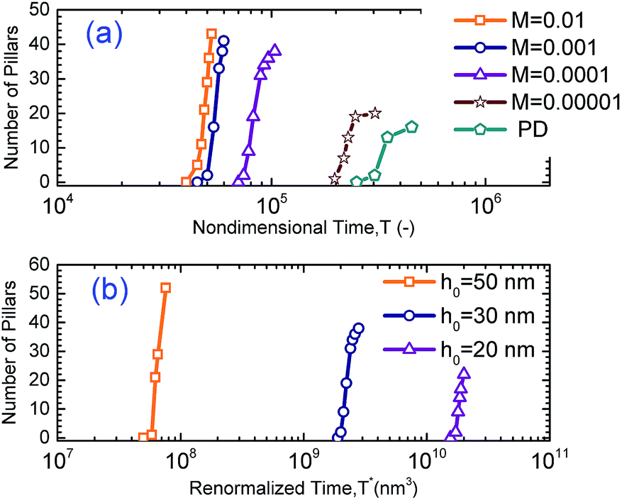
To further understand the potential of IL films for making smaller sized patterns in the EHD patterning process, molarity is increased. The effects of molarity and initial film thickness on the number of pillars in the EHD patterning process are presented in Fig. 8. For a fixed area, having a larger number of pillars means formation of smaller sized pillars on the IL film interface. The effect of ionic conductivity of IL films on the number of pillars and how fast they form is investigated by varying the molarities from M = 0.00001 to 0.01 mol L−1. The results are compared to those of a PD film of the same initial thickness, h0 = 30 nm, in Fig. 8(a). In Fig. 8(a) the number of pillars as a function of nondimensional time is plotted. The maximum value of each curve is the final (or maximum) number of pillars formed under quasi-stable conditions. Under the same applied voltage, the lowest final number of pillars is formed on the PD film (16 pillars). 20, 38, 41 and 43 final pillars are formed for the IL films with molarities of M = 0.00001, 0.0001, 0.001 and 0.01 mol L−1. When the molarity of IL films is increased ten times (from M = 0.00001 to 0.0001 mol L−1), the final number of pillars almost doubled, but further increase in molarity did not have a significant effect on the final number of pillars (Fig. 8(a)). In addition, it is apparent in Fig. 8(a) that the time gap between the formation of first and the final pillars in the IL film decreases with increasing molarity.
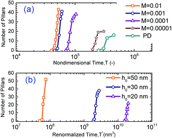 |
| | Fig. 8 Number of pillars formed with (a) molarity changes with a constant initial film thickness of h0 = 30 nm and (b) initial film thickness changes with constant molarity M = 0.0001 mol L−1. | |
Initial film thickness also affects the final number of pillars as shown in Fig. 8(b). Nondimensional time, T, is normalized by initial film thickness cubed; so a modified time is defined as T* = Th03, to cancel the effect of film thickness. Thus three initial film thicknesses of 20, 30 and 50 nm are selected at a constant molarity, M = 0.0001 mol L−1 and pillar formation as a function of T* is plotted in Fig. 8(b). Based on the time axis T*, films with higher initial thickness and the same interfacial tension and viscosity13 have faster time evolution which is similar to that observed in PD films.19 It is important to note that the above results show that the number of pillars formed on the interface from beginning to the final number of pillars is under quasi-steady conditions. It has been observed that a coarsening of structure in PD films with high initial thickness occurs in further later stages beyond these simulations.13,15 The coarsening of structure in IL films and related coarsening mechanism will be discussed later. The simulation results show that the number of pillars on the interface increases as the initial film thickness increases as shown in Fig. 8. The number and density of pillars for three initial thicknesses for both IL and PD films are given in Table 2. For the IL film the final number of pillars formed on the interface is increased significantly from 22 to 52 when the initial film thicknesses increased from 20 to 50 nm. The number of pillars formed in 1 μm2 area of the domain is defined as the density of pillars and is given in Table 2. The pillar density increases for both PD and IL films as a function of the initial film thickness with IL films having almost 5 times more pillar density than PD films.
Table 2 A summary of the number of pillars formed with changes of initial film thickness ratios in PD films and IL films with M = 0.0001 mol L−1
|
h
0 (nm) |
Final number of pillars |
Domain size (μm2) |
Density (pillars μm−2) |
| PD |
IL |
PD |
IL |
| 20 |
15 |
22 |
32.41 |
0.46 |
0.68 |
| 30 |
16 |
38 |
26.22 |
0.61 |
1.45 |
| 50 |
16 |
52 |
16.31 |
0.98 |
3.19 |
To gain further insight into the 2-D spatiotemporal evolution of an IL film, a film with 30 nm thickness and a molarity of M = 0.00001 mol L−1 is presented in Fig. 9(a–e) using interface height contours. Fig. 9(a) shows an early stage of the pattern formation process and contains an initial bicontinuous structure, isolated islands and a first columnar structure formation in one snapshot. Isolated islands from the previous stage are developed and converted to a columnar structure as shown in Fig. 9(b). The contact lines expanded on the top electrode and pillars are expanded in cross-section. Depletion of the liquid around pillars and formation of a ring-like depression around them are more obvious at this stage. The later stages of pillar formation are identified in Fig. 9(c) and (d) by dotted circles. Here coalescence of previously formed pillars is seen. Two neighboring pillars, dotted 1 and 2 in Fig. 9(c), merge and form one larger size pillar, 3 in image (d). The coalescence of neighboring pillars continues over time and pillars in Fig. 9(d) (dotted circle) merge to an even larger size pillar with an oval cross-section as shown in the dotted circle in Fig. 9(e).
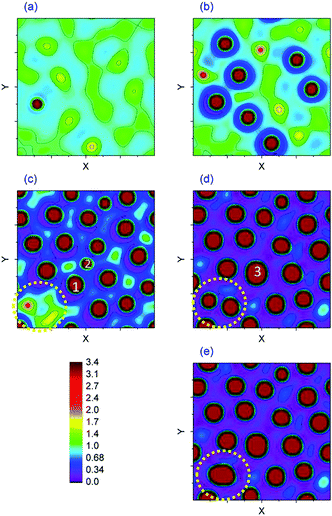 |
| | Fig. 9 2-D spatiotemporal evolution of a 30 nm IL film with a molarity of M = 0.00001 mol L−1. Nondimensional times, T, are (a) 197650, (b) 217980, (c) 247010, (d) 304670 and (e) 329150. | |
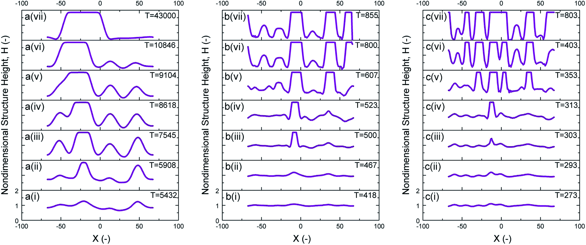
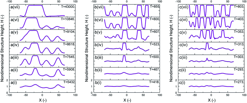
The dynamics and structure formation on the interface over time for PD and IL films can also be compared using 1-D spatiotemporal evolution of 50 nm IL films at Y = 0 (i.e. mid-plane). For an initial film thickness h0 = 50 nm, IL films with a with molarity of M = 0.001 and 0.0001 mol L−1 are compared to a PD film and the results are presented in Fig. 10. Increasing time is shown going upward in the subplots. Increasing the ionic conductivity of films (from zero in the case of PD films) results in pillars with smaller diameter and consequently denser structures as seen when comparing Fig. 10(a)–(c). The expansion of the contact line on the top electrode is also visible with this 1-D spatiotemporal evolution of the interface, Fig. 10a(ii–iii), b(iii–iv) and c(iv–v). Two mechanisms of pillar coalescence in the EHD patterning process are observed. The first one is Ostwald ripening of neighboring pillars in a PD film (Fig. 10a(iv)–a(vi)) in which an incomplete smaller pillar merges with a larger size pillar.13 The second mechanism is collision of neighboring pillars in an IL film with a molarity of M = 0.001 mol L−1 (Fig. 10c(v)–c(vii)). In this case, completely formed pillars with almost the same size merge and form larger size pillars. This type of coarsening is also observed in PD films, h0/d < 0.5, which have uniformly distributed pillars.15,27 An intermediate stage between the PD film and a highly ionic conductive film is shown in Fig. 10b(i)–b(vii) where the number of pillars formed is increased compared with the PD film.
 |
| | Fig. 10 1-D spatiotemporal evolution of 50 nm initial thickness at Y = 0. (a) PD film and IL films with (b) M = 0.0001 and (c) M = 0.001 mol L−1. | |
4. Conclusions
The system under study consists of two planar fluid layers, thin ionic liquid (IL) film and bounding media which are confined with flat electrodes. When a transverse electric field is applied to an IL film, the free ions move and accumulate close to the charged surfaces. This results in the formation of diffuse layers, called double layers, which are absent in perfect dielectric (PD) and leaky dielectric (LD) models. An electrostatic model is developed for confined IL films in contact with PD bounding media via coupling of linearized Poisson–Boltzmann and Laplace equations to obtain the electric potential distribution and consequently the net electrostatic pressure acting on the interface.
The developed IL model is not limited to the assumption of having an infinitesimally large or small electric diffuse layer that is inherited in the PD and LD models, respectively. This model is coupled to the nonlinear thin film equation and solved numerically to investigate the dynamics, instability and process of pattern formation in the EHD patterning process. Based on this model, ionic liquids are defined to be materials having properties between two limiting cases of PC and PD materials based on their ionic strength. IL films experience a much higher electrostatic pressure compared to similar PD films (with the same electric permittivity) and an increase in ionic strength results in higher electrostatic pressure. PD films are modeled first to investigate the accuracy of the numerical scheme and to provide a well known baseline case to compare the results with IL thin films. Finally IL films of various molarities are numerically simulated and the structure and number of pillars are compared to those of PD films.
Early stages of the pillar formation process in IL films are found to be similar to those of PD films and electrically induced instability growth is caused by negative diffusion. Pillars are initially formed on the random locations and enlarge in cross-section over time as the contact line expands on the top electrode. The pillar formation process occurs faster in IL films and is further accelerated with increasing ionic strength. Generally, smaller structures are found in IL films when compared to similar PD films and are increased with initial film height. In the case of increasing h0 from 20 to 50 nm, the IL film with M = 0.0001 mol L−1 gets 5 times more structures per 1 μm2 compared to a PD film.
References
-
W. Gilbert, de Magnete, Dover, New York, 1958, vol. 2, ch. 2, p. 89, 1600, translated by P. F. Mottelay in 1893 Search PubMed.
- L. Rayleigh, Philosophical Magazine Series 5, 1882, 14(87), 184–186 CrossRef.
- G. Taylor, Proc. R. Soc. London, Ser. A, 1966, 291(1425), 159–166 CrossRef.
- R. S. Allan and S. G. Mason, Proc. R. Soc. London, Ser. A, 1962, 267(1328), 45–61 CrossRef.
- D. Saville, Annu. Rev. Fluid Mech., 1977, 9, 321–337 CrossRef CAS.
-
W. B. Russel, D. A. Saville and W. R. Schowalter, Colloidal Dispersions, Cambridge University Press, Cambridge, UK, 1989 Search PubMed.
- J. S. Eow, M. Ghadiri, A. O. Sharif and T. J. Williams, Chem. Eng. J., 2001, 84, 173–192 CrossRef CAS.
- H. Stone, A. Stroock and A. Ajdari, Annu. Rev. Fluid Mech., 2004, 36, 381–411 CrossRef.
- J. Zeng and T. Korsmeyer, Lab Chip, 2004, 4, 265–277 RSC.
- S.-I. Jeong and J. Didion, J. Thermophys. Heat Transfer, 2008, 22(1), 90–97 CrossRef CAS.
- E. Schaffer, T. Thurn-Albrecht, T. P. Russell and U. Steiner, Nature, 2000, 403, 874–877 CrossRef CAS PubMed.
- R. V. Craster and O. K. Matar, Phys. Fluids, 2005, 17, 032104 CrossRef PubMed.
- N. Wu, M. E. Kavousanakis and W. B. Russel, Phys. Rev. E: Stat., Nonlinear, Soft Matter Phys., 2010, 81, 26306 CrossRef.
- P. Gambhire and R. M. Thaokar, Phys. Rev. E: Stat., Nonlinear, Soft Matter Phys., 2012, 86, 036301 CrossRef CAS.
- R. Verma, A. Sharma, K. Kargupta and J. Bhaumik, Langmuir, 2005, 21, 3710–3721 CrossRef CAS PubMed.
- P. D. S. Reddy, D. Bandyopadhyay and A. Sharma, J. Phys. Chem. C, 2010, 114, 21020–21028 CAS.
- S. Roy, D. Biswas, N. Salunke, A. Das, P. Vutukuri, R. Singh and R. Mukherjee, Macromolecules, 2013, 46, 935–948 CrossRef CAS.
- S. Srivastava, P. D. S. Reddy, C. Wang, D. Bandyopadhyay and A. Sharma, J. Chem. Phys., 2010, 132, 174703 CrossRef PubMed.
- A. Atta, D. G. Crawford, C. R. Koch and S. Bhattacharjee, Langmuir, 2011, 27, 12472–12485 CrossRef CAS PubMed.
- D. A. Saville, Annu. Rev. Fluid Mech., 1997, 27–64 CrossRef.
- K. Mondal, P. Kumar and D. Bandyopadhyay, J. Chem. Phys., 2013, 138, 024705 CrossRef PubMed.
- D. W. Lee, D. J. Im and I. S. Kang, Langmuir, 2013, 29, 1875–1884 CrossRef CAS PubMed.
- X.-F. Wu and Y. A. Dzenis, J. Phys. D: Appl. Phys., 2005, 38, 2848 CrossRef CAS.
- E. K. Zholkovskij and J. H. Masliyah and J. Czarnecki, J. Fluid Mech., 2002, 472, 1–27 CAS.
- E. K. Zholkovskij, J. H. Masliyah, V. N. Shilov and S. Bhattacharjee, Adv. Colloid Interface Sci., 2007, 134135, 279–321 CrossRef PubMed.
- P. Gambhire and R. Thaokar, Phys. Rev. E: Stat., Nonlinear, Soft Matter Phys., 2014, 89, 032409 CrossRef.
- C. Y. Lau and W. B. Russel, Macromolecules, 2011, 44, 7746–7751 CrossRef CAS.
- L. F. Pease and W. B. Russel, Langmuir, 2004, 20, 795–804 CrossRef CAS.
- H. Nazaripoor, C. R. Koch and S. Bhattacharjee, Langmuir, 2014, 30, 14734–14744 CrossRef CAS PubMed.
-
J. H. Masliyah and S. Bhattacharjee, Electrokinetic and Colloid Transport Phenomena, Wiley-Interscience, Hoboken, NJ, 2006 Search PubMed.
- M. B. Williams and S. H. Davis, J. Colloid Interface Sci., 1982, 90, 220–228 CrossRef CAS.
- R. W. Atherton and G. M. Homsy, Chem. Eng. Commun., 1976, 2, 57–77 CrossRef.
-
J. N. Israelachvili, Intermolecular and Surface Forces, Academic Press, Burlington, MA, 2011 Search PubMed.
-
L. D. Landau and E. M. Lifshitz, Electrodynamics of Continuous Media, Pergamon Press, 1960 Search PubMed.
- A. Oron, S. H. Davis and S. G. Bankoff, Rev. Mod. Phys., 1997, 69, 931–980 CrossRef CAS.
- A. Sharma and R. Khanna, Phys. Rev. Lett., 1998, 81(16), 3463–3466 CrossRef CAS.
- M. Z. Bazant, B. D. Storey and A. A. Kornyshev, Phys. Rev. Lett., 2011, 106, 046102 CrossRef.
-
E. J. W. Verwey and J. T. G. Overbeek, Theory and Stability of Lyophobic Colloids, Elsevier, Amesterdam, 1948 Search PubMed.
- M. Polat and H. Polat, J. Colloid Interface Sci., 2010, 341, 178–185 CrossRef CAS PubMed.
- F. H. Harlow and J. E. Welch, Phys. Fluids, 1965, 8, 2182–2189 CrossRef PubMed.
- C. Hirt and B. Nichols, J. Comput. Phys., 1981, 39, 201–225 CrossRef.
- H. Tian, J. Shao, Y. Ding, X. Li and H. Liu, Langmuir, 2013, 29, 4703–4714 CrossRef CAS PubMed.
- Q. Yang, B. Q. Li and Y. Ding, Soft Matter, 2013, 9, 3412–3423 RSC.
- K. E. Brenan and L. R. Petzold, SIAM J. Numer. Anal., 1989, 26(4), 976–996 CrossRef.
|
| This journal is © The Royal Society of Chemistry 2015 |
Click here to see how this site uses Cookies. View our privacy policy here. 
 Open Access Article
 This Open Access Article is licensed under a
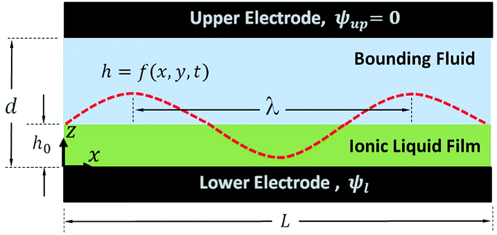
 ,
,  ,
,  and
and 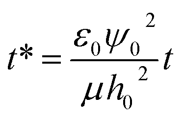 ) resulting in:
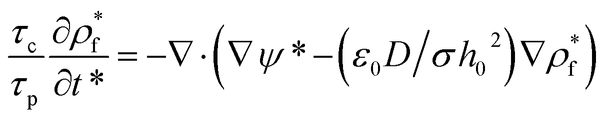

 ) at the interface. Eqn (11b) represents conservation of ions within the IL film and is used to find the reference potential, ψref. In this study the Debye Hückel approximation26,30 is used to linearize the Poisson equation transforming eqn (11a) and (11b) to:
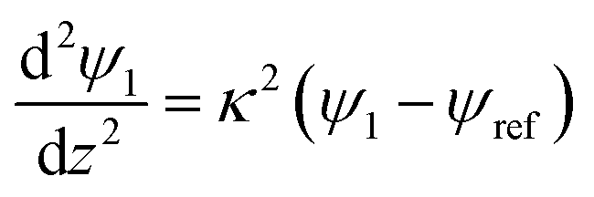
 is the inverse of Debye length. Solving eqn (10), (12a) and (12b) results in the electric potential distribution within PD and IL layers as follows:


 . This gradient is called the spinodal parameter and film instability due to this force is called spinodal instability.15 At a given location, when
  , a fluid flows from regions with lower thickness to higher thickness (negative diffusion) leading to growth of instabilities. To investigate the instability of an IL film subjected to an electric field, the term ϕ in eqn (3) is simplified to include only ϕE as the electrostatic component since this is dominant compared to other interactions for the EHD patterning.15 The variations of electrostatic conjoining pressure and the spinodal parameter with interface height for IL films of different molarities are shown in Fig. 4. A negative value of ϕE shows that the electrostatic force pushes the interface toward the upper electrode, often called disjoining force. By increasing the film thickness the electrostatic force is also increased for all three molarity values. Films with higher ion concentration, M = 0.01 and 0.001 mol L−1, experience higher electrostatic forces compared to the low concentration case of M = 0.00001 mol L−1. This difference is more apparent at higher film thicknesses (h0 > 50 nm), i.e. thicker films experience a higher force (more negative) than the thinner ones. This force accelerates growth of instabilities at initial stages to enhance the growth rate of structures at later stages.