On-chip ultrasonic sample preparation for cell based assays

Abstract

We demonstrate an acoustophoresis method for size-based separation, isolation, up-concentration and trapping of cells that can be used for on-chip sample preparation combined with high resolution imaging for cell-based assays. The method combines three frequency-specific acoustophoresis functions in a sequence by actuating three separate channel zones simultaneously: zones for pre-alignment, size-based separation, and trapping. We characterize the mutual interference between the acoustic radiation forces between the different zones by measuring the spatial distribution of the acoustic energy density during different schemes of ultrasonic actuation, and use this information for optimizing the driving frequencies and voltages of the three utilized ultrasonic transducers attached to the chip, and the flow rates of the pumps. By the use of hydrodynamic defocusing of the pre-aligned cells in the separation zone, a cell population from a complex sample can be isolated and trapped with very high purity, followed by dynamic fluorescence analysis. We exemplify the method's potential by isolating A549 lung cancer cells from red blood cells with 100% purity, 92% separation efficiency, and 93% trapping efficiency resulting in a 130× up-concentration factor during 15 minutes of continuous sample processing through the chip. Furthermore, we demonstrate an on-chip fluorescence assay of the isolated cancer cells by monitoring the dynamic uptake and release of a fluorescence probe in individual trapped cells. The ability to combine isolation of individual cells from a complex sample with high-resolution image analysis holds great promise for applications in cellular and molecular diagnostics.

---

Introduction

Sample preparation is a crucial step in many cell-based assays. Such preparation may include purification and up-concentration of a certain cell type from a complex sample such as blood, often including time-consuming manual steps prior to the analysis.¹ The conventional cell separation techniques rely on size, density and differential expression of surface antigens to isolate desired cell populations, including density gradient centrifugation,² preferential lysis of red blood cells, Ficoll-Hypaque density gradient centrifugation,³ porous filters, and cell filtration.⁴ These macro-scale methods are labor-intensive, non-standardized, and require large samples. After the separation, additional steps such as pipetting, cell staining and microscopic inspection are needed for analysis – steps that are time consuming. Microfluidics has the potential to overcome the shortcomings associated with macroscale isolation methods as well as integrating several of the critical steps in the analysis. Consequently, microfluidic technologies are expected to have increasing impact on the sorting, handling, and analysis of mammalian cells. Lab-on-a-chip-based platforms are attractive alternatives for this purpose, with the possibility to integrate and automate the sample preparation with on-chip cell assays,⁵e.g. by exposing cells to different reagents followed by on-chip live-cell imaging.⁶ However, while some of the standard sample preparation steps are available in the automated on-chip format, such as the centrifuge-on-a-chip,⁷ there are still only few methods available offering a complete, seamless integration of multiple sample preparation steps performed in a sequence on chip. A potential chip-based technology for multiple-step cellular sample preparation is acoustophoresis, i.e. manipulation of suspended cells into the pressure nodes of an ultrasonic standing wave. Acoustophoresis is today a widely used method in microfluidics with benefits such as low cost,⁸ good separation efficiency⁹ and long-term biocompatibility¹⁰ even at high acoustic pressures.¹¹ The method has shown to be useful in both cell-based^12,13 and bead-based^14,15 assays. In addition, surface acoustic waves (SAW) is an emerging technology for sample preparation purposes such as mixing and translation of fluids, and sorting, separation, filtration and washing of cells.^16–18

However, reports on acoustophoresis until today have either used the method for continuous-flow separation/focusing of cellular components into different outlet channels in a chip,^9,19 or for up-concentration, aggregation and retention of cells at a certain trapping site inside the chip.^20–22 In this paper, we demonstrate a novel sample preparation approach based on multi-step acoustophoresis for the size-based separation, isolation and up-concentration of cells, followed by fluorescence-based microscopy analysis of cellular dynamics.

In order to realize multi-step acoustophoresis including both continuous separation and trapping of cells in a single microfluidic chip, it is important to spatially separate the acoustic resonances into different channel segments and minimize overlaps of the resonating fields.²³ Here, the difficulty is related to the spurious three-dimensional acoustic resonance modes that always appear to some extent in microchannels,²⁴ even if a one-dimensional resonance was initially intended. In the present paper, we demonstrate a novel three-step acoustophoresis method for size-based separation, isolation and up-concentration of cancer cells (A549 lung cancer cell line) from red blood cells (RBCs). The method uses three ultrasound transducers, each operating at a specific frequency matching a resonance condition in one channel segment. We measure the spatial distribution of acoustic energy densities in the different channel segments, we quantify the separation and trapping efficiencies of A549 cells from RBCs at different flow rates, and we compare with the corresponding separation efficiency when using polymer beads of similar sizes. Furthermore, we demonstrate on-chip processing of the isolated and up-concentrated cancer cells by the addition of different reagents, here exemplified by the viability probe calcein-AM and the lysis buffer saponin. Our results show that the three-step acoustophoresis method can be used for on-chip sample preparation in applications using fluorescence-based cellular analysis.

Materials and methods

Microbead suspensions

A mixture of green-fluorescent 10 μm polystyrene beads (Fluoro-Max, Fisher Scientific, USA) and non-fluorescent 5 μm polyamide beads (Flow Doppler Phantoms, Danish Phantom Design, Denmark) was used for the initial characterization of the device and method. A concentration ratio of 1 : 1000 of 10 μm and 5 μm beads, respectively, was used to simulate rare cell conditions. For the acoustic energy density measurements, we used the 5 μm beads at high concentration. All bead suspensions were diluted in Milli-Q water with 0.01% Tween 20.

Cell line, culture and labeling

In order to evaluate the method's potential for size-based cell separation and up-concentration, we used a mixture of two different cell types: A549 human lung cancer cells (adenocarcinomic human alveolar basal epithelial cells, average diameter 10 μm), and RBCs (red blood cells, with an average volume corresponding to a sphere with diameter 5 μm). The A549 cells were cultured in RPMI-1640 (SH30027, Thermo Scientific, USA) supplemented with 10% fetal bovine serum (SV30160, Thermo Scientific, USA), and 100 U ml⁻¹ penicillin–100 μg ml⁻¹ streptomycin, 1× non-essential amino acids and 1 mM sodium pyruvate. After two days of culture, the cells were trypsinized and washed by centrifugation (1700 RPM in 3 min). Blood was acquired from anonymous healthy donors, and RBCs were separated from the rest of blood cells using the Ficoll separation technique (GE Healthcare Europe GmbH, Germany). RBCs were taken and diluted in different ratios in DPBS (Thermo Scientific, USA). Then the A549 cells were spiked into these solutions.

The fluorescent probe calcein green AM (Invitrogen, Carlsbad, CA, USA) was used for monitoring the cell viability. To pre-label the A549 cells, the cells were incubated with 2 μM of calcein-AM in RPMI-1640 at 37 °C for 30 minutes. The dye was then removed by washing in RPMI-1640 after which 2.5 ml of DPBS/modified was added at 37 °C. We also performed on-chip labelling using pre-heated 5 μM calcein-AM in RPMI-1640 at 37 °C.

Microfluidic chip and flow system

The chip, shown in Fig. 1, consists of a fluid channel with varying widths etched through a 0.11 mm silicon layer, which is sandwiched between two glass layers, 0.2 mm (bottom) and 1.10 mm (top). The layer thicknesses, as well as the optical transparency of the chip, were chosen for making the method compatible with high-resolution optical microscopy. The channel has several branches, in total eight inlets and outlets (cf.Fig. 1b). In this work, we used one inlet channel and three outlet channels (marked in green in Fig. 1b), and kept the other inlets/outlets blocked (marked with a red “X” in Fig. 1b). The fluid was driven through the channels via suction from the outlets: one syringe pump connected to the center outlet to the right driven at either 0.5 μl min⁻¹ or 1 μl min⁻¹, and another syringe pump connected to the two side outlets in the center of the chip driven at 2 × 2 μl min⁻¹ (two parallel syringes mounted in this pump). In this way, we were able to accurately control the flow rates going in the center and at the sides at the trifurcation point in the center of the chip, and keep them stable over time. The different segments in the channel that were driven at an ultrasound resonance were “Zone 1” (0.33 mm wide and 6.0 mm long), “Zone 2” (0.50 mm wide and 8.8 mm long) and “Zone 3” (expansion chamber with rounded walls; 1.43 mm maximum width and 3.63 mm long), cf.Fig. 1b and 2.

Fig. 1 (a) Schematic cross-section view of the microchip device (not to scale). The chip consists of a silicon layer (dark gray) sandwiched in between of two glass layers (light gray). It is actuated by (b): three different ultrasound transducers, 4.45 MHz (Zone 1), 1.39 MHz (Zone 2), and 2.78 MHz (Zone 3). The frequencies are selected to generate two pressure nodes in Zone 1, one pressure node in Zone 2, and a multitude of pressure nodes in Zone 3. In the upper panel in (b), the channel dimensions are shown in gray (mm), and the different zones are marked in colors. Two of the transducers (1.39 MHz and 4.45 MHz) used backing layers, as illustrated in (a), while the 2.78 MHz transducer was air-backed. Two suction-mode syringe pumps were used: one connected to the two outlets between Zone 2 and Zone 3, and one connected to the outlet to the right, after Zone 3.

Fig. 2 Conceptual illustration of the three-step acoustophoresis method. Cells or beads are pre-aligned into two acoustic pressure nodes in Zone 1 (4.45 MHz and 9 V_pp actuation), followed by size-based separation of larger cells or beads into one node in Zone 2 (1.39 MHz and 16 V_pp actuation), and finally isolation, retention and up-concentration of the larger cells or beads in Zone 3 (2.78 MHz and 10 V_pp actuation).

Ultrasonic transducers

Three transducers based on circular and rectangular piezoceramic plates (Pz-26, Ferroperm, Denmark) with different resonance frequencies were used to excite the three zones (see Fig. 1b and Table 1): a pre-alignment transducer operating at 4.45 MHz for producing two focused bands in Zone 1 (one full wavelength across the width, w), a separation transducer operating at 1.39 MHz for producing one focused band in Zone 2 (one half wavelength across the width, w), and a trapping transducer operating at 2.78 MHz for producing a multi-node trapping pattern in Zone 3. The zones and standing-wave patterns are illustrated in Fig. 2. The pre-alignment and the separation transducers were designed with epoxy-glue backing layers to enable frequency tuning within a wider band than possible with transducers without backing layers, while the trapping transducer was air-backed for fixed-frequency operation. The electrical resonances of the transducers were measured with an impedance analyzer (Model 16777k, SinePhase Instruments GmbH, Moedling, Austria), see Table 1. As seen in the table, the transducers with backing layers had bandwidths about 10% of the center frequency, compared to about 0.5% for the transducer without backing layer. In practice, it is possible to use driving frequencies within about twice the (full width half maximum) bandwidth, as seen for the separation transducer. However, the driving frequency maximizing the energy density in the fluid channel is generally not identical with the electrical resonance frequency of the transducers.²⁵ The transducers were attached to the chip with a water-soluble adhesive gel (Tensive, Parker Laboratories, USA), and driven by separate function generators (DS345, Stanford, USA). For the separation transducer who had the lowest Q value, we used an RF amplifier (75A250, Amplifier Research, USA), for enabling actuation voltages above 10 V_pp.

Table 1 Properties of the ultrasonic transducers used for exciting the three different channel zones

Transducer	Experimental driving frequency	Backing layer	Electr. imp. center frequency	Electr. imp. bandwidth	Electr. imp. Q value
Zone 1: pre-alignment	4.45 MHz	Yes	4.33 MHz	432 kHz	10
Zone 2: separation	1.39 MHz	Yes	1.56 MHz	174 kHz	9
Zone 3: trapping	2.78 MHz	No	2.80 MHz	15 kHz	184

---

Temperature sensing

The temperature was measured at the top glass layer with a T-type (copper-constant) and Teflon-insulated micro thermocouple (Model IT-21, Physitemp Instruments, USA). Temperature data was automatically monitored with the accuracy of ±0.1 °C (Dostmann Electronic GmbH P655-LOG, Germany). During all experiments the temperature was stable within 1 °C, and thus no temperature regulation²⁶ was needed.

Imaging

The microchannel was imaged by an inverted microscope (Axiovert 40, Zeiss, Germany) equipped with either a 10×/0.25NA objective (Zeiss, Germany), or a 20×/0.40NA objective (Olympus, Japan). We used two different cameras: a Sony α7 (Sony, Japan) for video recording, and a Zeiss AxioCam HSC (Zeiss, Germany) for fluorescence still images. For the separation and trapping efficiency experiments, we used manual counting of beads or cells into each of the three channels after Zone 2 (separation efficiency) and in and out of Zone 3 (trapping efficiency).

Measuring the acoustic energy density

For in situ measurements of the acoustic energy density in the channel, we used a light transmission method as described previously.^27,28 In brief, the method summarizes the light intensity transmitted through a certain segment of the fluid channel filled with a high concentration of 5 μm beads. When the beads move into the pressure nodes of the ultrasonic standing wave, the transmitted light intensity increases, and this increase as a function of time is used for calculating the acoustic energy density. Here, we injected 5 μm beads at a concentration of approx. 10⁸ ml⁻¹, and after stopping the flow the transducers were actuated and the light intensity was extracted from the recorded images (600 frames during 30 s) and inserted into the model described in ref. 27.

Results

Spatial distribution of the acoustic energy density at multi-frequency operation

In a first set of experiments, we were interested in measuring the distribution of acoustic energy density, E_ac, inside and outside the first two zones (cf.Fig. 2), when operating one or two ultrasonic transducers. This is important for being able to separate the cell manipulation functions to the different zones without mutual interference between each function. The light-intensity method for estimating E_ac is based on a 1D model and only takes into account the acoustic energy density causing radiation forces acting across the width w of the fluid channel (cf.Fig. 1). Previously, we have used the model in half-wave resonators, corresponding to one acoustic pressure node of the standing wave.^27,28 In this work, we expanded the model to also handle multi-node resonances as used in the first zone (pre-alignment, two nodes, cf.Fig. 2). The transducers for Zone 1 (4.45 MHz) and Zone 2 (1.39 MHz) were driven at 9 and 16 V_pp, respectively. These values were the optimal driving voltages for the cell and bead separation experiments as described below, i.e. for maximizing the separation efficiencies. The energy density was measured when driving one transducer at a time (Fig. 3a and b), as well as when driving both simultaneously (Fig. 3c).

Fig. 3 Measurements of the spatial distribution of the acoustic energy density in Zone 1 (0 mm < x < 6 mm) and Zone 2 (6 mm < x < 15 mm) when actuation one transducer at the time (a and b), or two transducers simultaneously (c). (a) Actuation of the pre-alignment transducer (Zone 1) at 4.45 MHz. (b) Actuation of the separation transducer (Zone 2) at 1.39 MHz. (c) Actuation of both the pre-alignment and separation transducers (Zone 1 and 2) transducer at 4.45 MHz and 1.39 MHz, respectively. The diagrams show the acoustic energy densities when selecting driving voltages for optimal separation performance. The standard deviations correspond to three repetitions of each experiment. The plotted energy densities are the components responsible for particle manipulation in the y direction (along the channel width), since the utilized method for measuring energy density is a one dimensional method. Error bars correspond to ±1SD from three repetitions of the experiment.

As seen in Fig. 3, while there is no measurable energy density outside Zone 2 when operating the separation transducer (Fig. 3b), there is a significant amount of energy density outside Zone 1 (approx. 50% of the average E_ac inside Zone 1) when operating the pre-alignment transducer (Fig. 3a). This “leakage” of resonance is a frequently occurring problem in acoustophoresis,²³ in particular in multi-node resonance channels,²⁴ and is difficult to avoid when exciting a channel segment that is narrower than surrounding segments. The resonance leakage occurred for any driving frequency within the pre-alignment transducer bandwidth (cf.Table 1), which made it difficult to optimize the separation by frequency tuning only. To overcome this problem, we decided to operate the separation transducer at a voltage level producing a much higher acoustic energy density in Zone 2, relative to the energy density produced by the pre-alignment transducer in Zone 1, and then to adjust the separation threshold for the sizes of beads and cells used with the flow rates of the two suction pumps. This strategy is confirmed in Fig. 3c, where we see that the leakage of the pre-alignment resonance has no effect on the separation resonance when operating both transducers simultaneously. Neither did the trapping transducer influence the energy densities inside Zones 1 or 2.

Bead separation efficiency

After the optimization of driving frequencies and voltages in the first two zones, we measured the performance of pre-alignment and separation of 10 μm beads from 5 μm beads mixed in a concentration ratio 1 : 1000, respectively. The separation principle is illustrated in Fig. 2. The suction pumps were operated to produce in total 5.0 μl min⁻¹ flow rates: 1.0 μl min⁻¹ in the center channel between Zone 2 and Zone 3, and 2.0 μl min⁻¹ in each side channel after Zone 2 (cf.Fig. 2). The separation efficiency is shown in Fig. 4. With the chosen flow settings, we were able to focus on average 83.4% of the 10 μm beads into the center channel between Zone 2 and Zone 3, while 16.6% were washed out into the other outlets after Zone 2. The flow and transducer voltage settings were here selected by pre-calibration for minimizing contamination of the smaller beads (5 μm) into the trapping chamber (Zone 3), instead of maximizing the injection of larger beads into Zone 3. Thus, although we lose 16.6% of the 10 μm beads, we have for this flow/voltage setting 0% contamination of 5 μm beads into Zone 3.

Fig. 4 Separation efficiency of 10 μm polystyrene beads from 5 μm polystyrene beads when using 1.0 μl min⁻¹ flow rate in the center channel after Zone 2, and 2.0 + 2.0 μl min⁻¹ flow rates in the two side channels after Zone 2. The experiment was optimized for minimizing the number of 5 μm beads entering Zone 3. Error bars correspond to ±1SD from three repetitions of the experiment.

Cell separation efficiency

As proof of principle for cell based applications, measurements were performed for separation of lung cancer cells from RBCs. Here, the sample consisted of 5 × 10⁵ RBCs per μl and 4 × 10⁵ calcein-labeled A549 cells per μl diluted in DPBS buffer. The result is seen in Fig. 5. In these experiments, we used a concentration ratio of approx. 1 : 1, because our quantification method based on manual image analysis of recorded video sequences did not allow high RBC concentrations when counting the number of A549 cells going into the side channels after Zone 2. When using the same flow settings as for the bead separation measurements (cf.Fig. 4; total flow rate 5 μl min⁻¹, out of which 1 μl min⁻¹ into the center channel after Zone 2), we were able to focus 71.4% of the A549 cells into the center channel, while losing 28.6% into the side channels after Zone 2 (still with 0% contamination of RBCs into the center channel). Thus, the cell separation efficiency was slightly lower than the corresponding bead separation efficiency, which is expected since cells do not have as uniform sizes and acoustic properties as the beads. However, the separation efficiency is a function of the chosen flow rates. As seen in Fig. 5, when the flow rate in the center channel after Zone 2 was decreased from 1.0 μl min⁻¹ to 0.5 μl min⁻¹, the separation efficiency increased to 92.4% focused A549 cells (7.6% lost). Importantly, although flow rate at the center channel was reduced by half, the total sample processing rate only decreased from 5.0 μl min⁻¹ to 4.5 μl min⁻¹. Hence, a dramatic increase in capture efficiency (from 76% to 92%) without the need to compromise on sample processing speed.

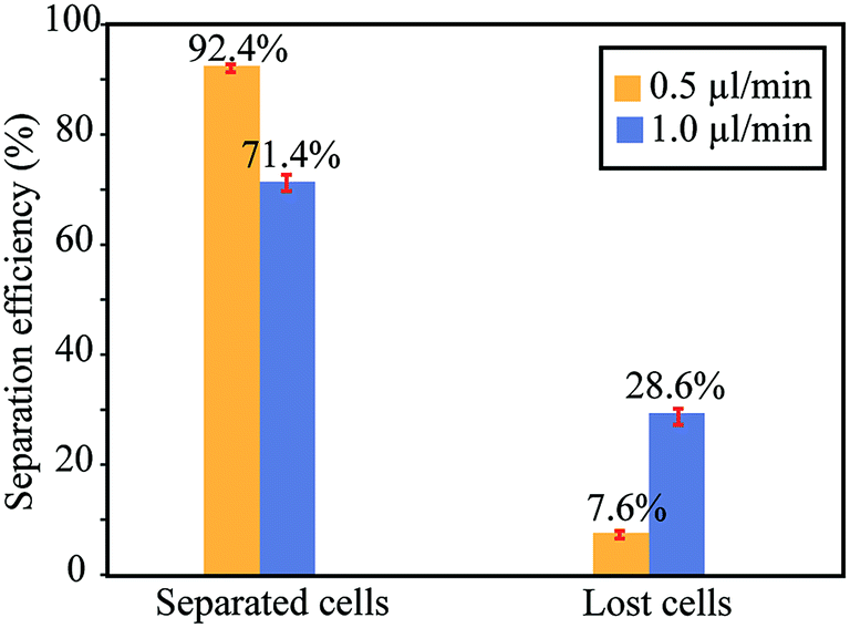Fig. 5 Separation efficiency of A549 cancer cells from red blood cells at two different flow rates in the center channel after Zone 2. The blue bars correspond to the same actuation and flow parameters as in Fig. 4, while the yellow bars show the separation efficiency when lowering the flow rate in the center channel after Zone 2 to 0.5 μl min⁻¹, while keeping the flow rates in the two side channels after Zone 2 to 2.0 + 2.0 μl min⁻¹. Thus, the total injected flow rate into the chip is 4.5 μl min⁻¹ (yellow bars) and 5.0 μl min⁻¹ (blue bars). Error bars correspond to ±1SD from three repetitions of the experiment.

Cell separation, isolation, up-concentration and trapping

After selecting suitable driving parameters for the size-based cell separation (two transducers in operation), we expanded the experiments by studying trapping and up-concentrating the isolated cells in Zone 3 during actuation with the third transducer. Microscopic views from the method is shown in Fig. 6, where A549 cells are separated from RBCs and trapped using the A549 : RBC concentration ratio 1 : 100 (Fig. 6a). As seen in Fig. 6b (the trapping chamber, Zone 3) and in the ESI video S1,† the cells are typically trapped in multiple clusters inside the chamber. This is a result of driving the relatively large trapping chamber at an ultrasound multi-node resonance in two dimensions. However, single cells could be imaged with the microscope independently if they were clustered or not.

Fig. 6 Microscopic view from the chip during an experiment. (a) Sized-based separation of A549 cancer cells from RBCs after Zone 2. The RBC : cancer cell ratio is 100 : 1. (b) Trapping and up-concentration of the separated cancer cells in Zone 3.

For quantifying the trapping efficiency, we used the same flow settings (2 + 0.5 + 2 μl min⁻¹) and cell concentrations as in the previous experiment (cf.Fig. 4, yellow bars). The trapping efficiency was measured by manually counting the number of A549 cells that entered and escaped from the trapping chamber (Zone 3) while operating the trapping transducer at 2.78 MHz and 10 V_pp. For this flow setting, between 100 and 200 A549 cells per minute entered Zone 3. As seen in Fig. 7, we were able to isolate and trap 93.1% of the A549 cells while losing 6.9% (escaping out from Zone 3). This quantification was performed during 15 min, resulting in an up-concentration factor of >130 with the measured separation efficiency (92.4%) and trapping efficiency (93.1%).

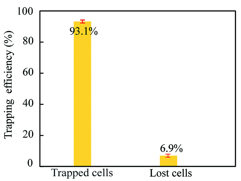Fig. 7 Trapping efficiency of isolated A549 cancer cells in Zone 3 when using the same flow settings as for the yellow bars in Fig. 5. Error bars correspond to ±1SD from three repetitions of the experiment.

On-chip staining and lysis of individual isolated cells

In the last set of experiments, we demonstrate how to use the method for analyzing the isolated cells with microscopy when they are exposed to different reagents. After completing the isolation and up-concentration of un-stained A549 cells, we switched from the cell sample connected to the inlet of the chip to a buffer containing the viability probe calcein-AM (5 μM). Here, we could prevent the injection of further A549 cells into the trapping chamber by simply turning off the separation transducer (1.39 MHz), resulting in that all pre-aligned cells from Zone 1 are guided out through the side channels after Zone 2, and only clear buffer with reagents entered Zone 3 with the already isolated and trapped A549 cells. The dynamics of uptake of calcein from individual trapped cells could then be monitored with fluorescence microscopy, as demonstrated in Fig. 8. Finally, we introduced two different reagents in a sequence: first calcein-AM followed by the lysis probe saponin (1%). The dynamics of uptake and saponin-induced release of calcein from individual cells is quantified in Fig. 9. Here, we selected three cells trapped at different positions inside the chamber, as indicated by the different colors. We observed that the calcein uptake time is about 40 min, while the saponin-induced lysis time is between 6 and 12 min. These time constants are comparable to what is used in standard protocols, although slightly longer due to the gradual increase in reagent concentration in the chamber caused by the parabolic flow profile. We also observed the approx. 5 minutes delay of the initiation of uptake or release between the three differently located cells (approx. 1.5 mm distance in between). These sets of experiments show the possibility of integrating high resolution imaging with on-chip sample preparation steps, which should open up possibilities for many different applications.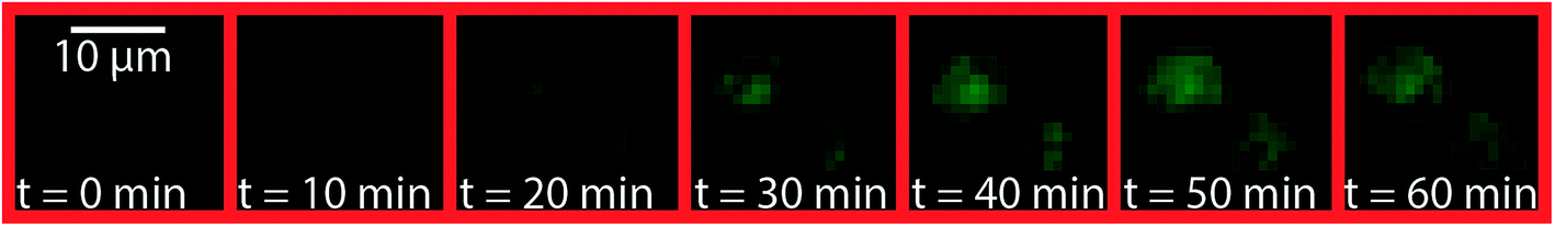

Fig. 8 Demonstration of dynamic monitoring of the uptake of the viability probe calcein-AM (5 μM) in individual trapped A549 cancer cells in Zone 3.

Fig. 9 Quantification of the dynamics of uptake (a) and saponin (1%)-induced release (b) of calcein-AM (5 μM) in three individual A549 cells trapped in different parts of the trapping chamber (Zone 3). The flow rates are the same as in the separation and trapping experiments: 4.5 μl min⁻¹ injected flow, out of which 0.5 μl min⁻¹ is passing the trapping chamber (Zone 3).

Discussion

The present work is the first combination of size-based continuous separation and trapping of cells based on multi-step acoustophoresis. The purpose of the method is to perform on-chip sample preparation combined with cellular fluorescence analysis, by the use of a simple setup consisting of a glass–silicon chip, three ultrasound transducers and two syringe pumps.

When performing multi-step acoustophoresis in a single microfluidic chip, it is important to select driving frequencies for the different transducers that do not cause major interference between the acoustic radiation force fields in the channel. When using complex channel geometries, multi-node cavity resonances and multiple resonant zones, such interference is in practice impossible to avoid. However, in this study we solved the problem by selecting flow rates after the separation zone (Zone 2, cf.Fig. 1 and 2) with much lower rate in the center channel towards the trapping chamber relative the flow rates out in the side channels. Within Zone 2, this flow setting acted as a hydrodynamic defocusing of the beads and cells, competing with the acoustophoretic focusing. The hydrodynamic defocusing was also beneficial for the sample processing rate: the isolated and trapped cells were guided into the center channel towards Zone 3 with only approx. 10% of the total flow rate, while approx. 90% of the flow rate was led out through the side channels after Zone 2. The only drawback with this flow setting was the relatively long response times (up to 10 minutes) when exposing the isolated and trapped cells for different reagents, i.e., the time to fully exchange the medium in Zone 3. On the other hand, this response time could be improved in the future by the use of a smaller trapping chamber, e.g. a half-wave trapping chamber.²⁹ Such a smaller chamber would also lead to a single trapping position of up-concentrated cells, but with a much smaller loading capacity that for the chamber used in this study. Furthermore, our method uses acoustophoretic pre-alignment in the first step (Zone 1), instead of the commonly used hydrodynamic focusing method before the size-based separation step. This means that we do not start by diluting the sample, instead, we process non-diluted sample through all steps in the whole chip. Although acoustophoretic pre-alignment is generally more accurate than hydrodynamic pre-alignment, our method could be further improved in the future by adding a vertical acoustic resonance in the system which enables two-dimensional acoustophoresis.^25,30

In this study we used for the first time broadbanded ultrasonic transducers consisting of planar PZT plates with epoxy-glue-based backing layers. Such transducers are used in pulse-echo ultrasonic imaging (diagnostic ultrasound), but have to our knowledge not been used for acoustophoresis in microfluidic chips. On the contrary, most other groups use high-quality-factor, single-frequency transducers with air-backing for acoustophoresis. While this may be the optimal design for single-step, half-wave acoustophoresis in chips with simple channel geometries, it is not suitable for the multi-step acoustophoresis device we used in this work. The broadbanded transducers allowed us to fine-tune the driving frequencies within much wider ranges than possible with high-Q-factor transducers, in order to avoid mutual interference between the acoustic fields in the different zones in the chip. As demonstrated in this work, broadbanded transducers can be used in acoustophoresis without causing any significant heating or need for large signal amplifications. It should be noted, that one of the three transducers used in this study was not broadbanded (the trapping transducer). This air-backed transducer was used for exciting the trapping chamber. Here, we instead created a “broadbanded” chamber by choosing a chamber size (length and width) ≫ the acoustic wavelength. For such chamber geometries, almost any transducer frequency will create an ultrasound standing-wave resonance. Since it was not important to select a particular trapping pattern (something that was very important in the pre-alignment and separation zones), we could simply select a driving frequency that corresponded to a good transducer resonance.

We have demonstrated how to isolate and up-concentrate larger cells (here, A549 lung cancer cells) from smaller cells (here, RBCs) by a three-step on-chip acoustophoresis method. While the A549 cancer cell line and the RBCs were selected for proof-of-concept purposes, the method can easily be expanded to separate, concentrate and analyze any cell population based on size from other sample matrixes. The reported data demonstrates isolation with 100% purity and >130× up-concentration of A549 cells during 15 minutes. In total, >86% of the A549 cells processed during this time are retained (both separation efficiency and trapping efficiency was higher than 92%). We have tested the method for different concentration ratios of A549 cells and RBCs, ranging from 1 : 1000 to 1 : 1. The method performs well even for rare-cell conditions (concentration ratio 1 : 1000), but our manual on-chip quantification method used here was not applicable to such rare-cell conditions. It should also be noted that in this work, we have not studied isolation of cancer cells from whole blood, which is a more difficult task given the fact the circulating cancer cells (CTCs) are very rare and because of the smaller size difference between healthy leukocytes (WBCs) and cancer cells (relative the size difference between RBCs and cancer cells).

The benefit with on-chip isolation and up-concentration of cells is the possibility to perform direct high-resolution microscopy-based analysis of the trapped cells. In this study we demonstrated how to stain and lyse the A549 cells by adding two different reagents (calcein-AM and saponin) in a sequence. The calcein confirmed that the cell viability was intact after the acoustophoretic processing, but more importantly, the method enables dynamical studies of individual cell incubation with any compound of interest. In this study, we demonstrated individual uptake and release of calcein from three different cells. However, it is also possible to study the response from larger cell numbers (up to approx. 10⁴ isolated cells corresponding to the loading capacity of the trapping chamber).

Acknowledgements

We thank the Swedish Research Council, the EU FP-7 IMI RAPP-ID project, and Stockholms Läns Landsting for financial support.

References

1. A. J. Mach, O. B. Adeyiga and D. Di Carlo, Lab Chip, 2013, 13, 1011–1026.
2. L. Vettore, M. C. de Matteis and P. Zampini, Am. J. Hematol., 1980, 8, 291–297.
3. P. Madyastha, K. R. Madyastha, T. Wade and D. Levine, J. Immunol. Methods, 1982, 48, 281–286.
4. H. N. Chang, W. G. Lee and B. S. Kim, Biotechnol. Bioeng., 1993, 41, 677–681.
5. C. Rivet, H. Lee, A. Hirsch, S. Hamilton and H. Lu, Chem. Eng. Sci., 2011, 66, 1490–1507.
6. M. Wu, T. D. Perroud, N. Srivastava, C. S. Branda, K. L. Sale, B. D. Carson, K. D. Patel, S. S. Branda and A. K. Singh, Lab Chip, 2012, 12, 2823–2831.
7. A. J. Mach, J. H. Kim, A. Arshi, S. C. Hur and D. Di Carlo, Lab Chip, 2011, 11, 2827–2834.
8. A. Lenshof, M. Evander, T. Laurell and J. Nilsson, Lab Chip, 2012, 12, 684–695.
9. A. Lenshof, C. Magnusson and T. Laurell, Lab Chip, 2012, 12, 1210–1223.
10. M. Wiklund, Lab Chip, 2012, 12, 2018–2028.
11. M. Ohlin, I. Iranmanesh, A. E. Christakou and M. Wiklund, Lab Chip, 2015, 15, 3341–3349.
12. A. Lenshof, A. Jamal, J. Dykes, A. Urbansky, I. Åstrand-Grundström, T. Laurell and S. Scheding, Cytometry, Part A, 2014, 85, 933–941.
13. M. Wiklund, Cytometry, Part A, 2014, 85, 915–917.
14. J. Persson, P. Augustsson, T. Laurell and M. Ohlin, FEBS J., 2008, 275, 5657–5666.
15. M. Wiklund, S. Radel and J. J. Hawkes, Lab Chip, 2013, 13, 25–39.
16. X. Ding, P. Li, S. S. Lin, Z. S. Stratton, N. Nama, F. Guo, D. Slotcavage, X. Mao, J. Shi, F. Constanzo and T. Jun Huang, Lab Chip, 2013, 13, 3626–3649.
17. R. W. Rambach, V. Skowronek and T. Franke, RSC Adv., 2014, 4, 60534–60542.
18. G. Destgeer and H. Jin Sung, Lab Chip, 2015, 15, 2722–2738.
19. M. Antfolk, C. Antfolk, H. Lilja, T. Laurell and P. Augustsson, Lab Chip, 2015, 15, 2102–2109.
20. J. Svennebring, O. Manneberg, P. Skafte-Pedersen, H. Bruus and M. Wiklund, Biotechnol. Bioeng., 2009, 103, 323–328.
21. M. Evander and J. Nilsson, Lab Chip, 2012, 12, 4667–4676.
22. B. Hammarström, B. Nilsson, T. Laurell, J. Nilsson and S. Ekström, Anal. Chem., 2014, 86, 10560–10567.
23. O. Manneberg, S. M. Hagsäter, J. Svennebring, H. M. Hertz, J. P. Kutter, H. Bruus and M. Wiklund, Ultrasonics, 2009, 49, 112–119.
24. S. M. Hagsäter, A. Lenshof, P. Skafte-Pedersen, J. P. Kutter, T. Laurell and H. Bruus, Lab Chip, 2008, 8, 1178–1184.
25. O. Manneberg, J. Svennebring, H. M. Hertz and M. Wiklund, J. Micromech. Microeng., 2008, 18, 095025.
26. J. Svennebring, O. Manneberg and M. Wiklund, J. Micromech. Microeng., 2007, 17, 2469–2474.
27. R. Barnkob, I. Iranmanesh, M. Wiklund and H. Bruus, Lab Chip, 2012, 12, 2337–2344.
28. I. Iranmanesh, R. Barnkob, H. Bruus and M. Wiklund, J. Micromech. Microeng., 2013, 23, 105002.
29. O. Manneberg, B. Vanherberghen, J. Svennebring, H. M. Hertz, B. Önfelt and M. Wiklund, Appl. Phys. Lett., 2008, 93, 063901.
30. C. Grenvall, C. Antfolk, C. Zoffmann Bisgaard and T. Laurell, Lab Chip, 2014, 14, 4629–4637.

---

Footnote

† Electronic supplementary information (ESI) available. See DOI: 10.1039/c5ra16865a

---