Predictive calculation of carbon dioxide solubility in polymers

Abstract

The solubility of carbon dioxide in polymers has attracted great attention from scientists because it is an important application of green chemistry, and it is widely applied in extraction, separation and the preparation of new materials. In this work, a new solubility prediction model with both good accuracy and efficiency, called CEAPSO KHM RBF ANN, is developed. In the CEAPSO KHM RBF ANN model, an accelerated particle swarm optimization (APSO) algorithm with chaotic disturbance is employed to trim the radial basis function artificial neural network (RBF ANN) connection weights and biases in order to reduce the premature convergence problem, and the K-harmonic means (KHM) clustering method is used to tune the hidden centers and spreads of the radial basis function. The proposed model is employed to investigate the solubility of CO₂ in polymers including polypropylene, polystyrene, poly(vinyl acetate), carboxylated polyesters and poly(butylene succinate-co-adipate). The results indicate that the proposed model is an effective method for solubility prediction with better performance and higher efficiency compared with the other methods, and should contribute to the understanding of the phase behaviour of the gas/polymer system and for the design and optimization of processing techniques.

---

1. Introduction

Carbon dioxide (CO₂) has become the most popular green medium currently, and has been widely used as a solute or solvent in many fields including material modification, synthesis and processing because of its advantages like no toxicity, chemical inertness, nonflammability and easy accessability.^1–3 The solubility of CO₂ in polymers has been a subject of interest for chemical engineers for several decades, and it has also been applied in a wider application field, such as extraction, separation and the preparation of new materials and so forth.^4,5 To describe gas solubility in polymers, calculation models are often used.⁶ For example, thermodynamic models and intelligent models have been extended to describe phase behavior of a polymer solution. The thermodynamic methods consist of the equation of state, empirical equation and semi-empirical equation; while the intelligent calculation methods consist of an artificial neural network (ANN) and support vector machine.^7–12 Bakhbakhi¹³ applies the equation of state and an ANN to conduct a comparison of the calculation of solubility, and it turns out that the computational accuracy obtained through calculation by an ANN is higher. Pahlavanzadeh¹⁴ proves that a better effect in the calculation of solubility can be achieved by using an ANN; Mehdizadeh¹⁵ and Gharagheizi¹⁶ also conclude that an ANN has better performance in the prediction of solubility. Due to the good generalization ability, the radial basis function (RBF) ANN has been widely used for the prediction of solubility, but Khajeh¹⁷ summaries through comparison that the adaptive neuro-fuzzy inference system (ANFIS) has better performance in predicting solubility than that of the RBF ANN. In other words, the network parameters of the RBF ANN have a conclusive influence on the overall performance, and an optimization is necessary. As is known to all the parameter optimization of the ANN is a classical optimization problem, so many intelligent optimization algorithms have been used for optimization of the network parameters,¹⁸ such as a genetic algorithm,^19–21 simulated annealing,²² particle swarm optimization (PSO),^23,24 a tabu search,^25,26 a cuckoo search algorithm,²⁷ etc.

The PSO algorithm is a classical intelligence algorithm inspired by birds seeking food. It has many advantages, such as fewer adjustment parameters, convenient implementation, fast convergence speed, etc. And it has been broadly used for parameter optimization of ANNs. Liu²⁸ has successfully obtained the prediction model of the melt index of a fuzzy ANN by PSO; Lazzus²⁹ also successfully established the hybrid prediction model based on PSO and an ANN. However, PSO itself also has some defects, for example, poor search capability at a later period of optimization and easily falling into a local minimum. In order to improve the deficiencies, scientists have proposed many variants. Li^30–34 proposed several models and applied the chaos theory and self-adaption strategy in the improvement of PSO. The results show that the effects of prediction of the proposed models are pretty good.

In the past two years, a new variant called accelerated PSO (APSO) has been the simplest and a high efficiency algorithm with free parameters among so many variants, to which has been paid close attention by researchers. It has successfully solved many practical problems. Specifically, it is suitable for optimization of RBF ANN parameters. But it also has problems like easily falling into a local minimum. Given that, this article will discuss the integration of APSO and chaos theory to propose an improved algorithm, and apply the improved algorithm and K-harmonic means (KHM) clustering in the training of the RBF ANN. Consequently, it attempts to get a hybrid network model with both good accuracy and efficiency, and uses the model in the prediction of the solubility of CO₂ in polymers in this work.

2. Theory and experimental data

2.1 Chaos-enhanced accelerated particle swarm optimization

In recent years, APSO has become a new simplified variant of the PSO algorithm; it could accelerate the convergence using the global best only. In APSO, the velocity is abandoned in order to increase the convergence speed even further, thus there is no need to initialize the velocity.³⁵ Therefore, it is much simpler to implement. The position vector of a particle is updated as follows:

x_i^t+1 = (1 − c₁)x_i^t + c₁g_best + c₂r (1)

where x_i is the position vector, and g_best is the global extremum. r is a random vector, and c₁ and c₂ are often called acceleration coefficients.

The APSO is very efficient, but it also has problems like easily falling into a local minimum, and may miss some solutions sometimes. In fact, there is no need to keep the acceleration coefficients constant, and the varying acceleration coefficients are very advantageous, which may lead to the convergence speed-up. Therefore, in this work, we employ the Lorenze equations to generate a chaotic sequence for tuning the acceleration coefficients c₁ and c₂ of the APSO, and develop a new improved algorithm, called CEAPSO. The chaotic sequence is defined as follows:³⁶

where a, b, and r are the system parameters, and the Lorenze system can achieve a chaotic state completely when a, b, and r are set as 10, 8/3 and 28, respectively.³⁷ Given the dynamic properties of x(t) and y(t), the acceleration coefficients c₁ and c₂ are defined as follows:

The acceleration coefficients c₁ and c₂ can enhance the ability to escape a local minimum by tuning with the chaotic sequence, and at the same time increase the possibility of searching for a global extremum.

2.2 KHM cluster method

The KHM cluster method is an iterative process based on a cluster center. The objective function adopts the harmonic mean of the distance from all the sample points to each center of clustering, defined as:

In the formula, X = [x₁,…,x_n] is the sample data set, n is the number of the sample, k is the number of the cluster, and C = [c₁,…,c_n] is the vector quantity of the center of clustering.

The computational formulas of the degree of membership m(c_j/x_i) and weight w(x_i) between each sample data set and vector quantity of the center of clustering are:

where p is the input parameter, and it’s assumed as 2 in this article.³⁸

The updated formula of the vector quantity of the cluster center, c_j, is:

The KHM clustering algorithm will constantly iterate based on the vector quantity of the center of clustering and according to the original value, so as to make the value of the objective function gradually reduce until it is stable.

2.3 CEAPSO KHM RBF ANN

The RBF ANN is one of the classical forward neural networks, containing three layers: an input layer, a hidden layer and an output layer. This article proposes a hybrid RBF ANN model based on the CEAPSO and KHM cluster algorithm, called CEAPSO KHM RBF ANN. The output of the network model is defined as:

In the formula, w_i is the connection weight of the i^th hidden node. x_k (1 ≤ k ≤ n) is the number k input vector, c is the number of nodes at the hidden layer, and g is the activation function.

The training process of the RBF ANN can be regarded as a process of optimization of the center, spread and connection weight, that is, to optimize c_i, σ_i and w_i. In this article, we adopt the KHM algorithm to optimize the center and spread of the radial basis function, defined as:

KHM(C_{basis function},C_cluster) (9)

In that, C_cluster is the center of clustering in the KHM algorithm, and C_{basis function} is the center of the radial basis function. The center of each radial basis function will update according to the center of clustering.

In the meantime, the connection weight and bias of the hidden layer and output layer in the RBF ANN will be optimized by means of the CEAPSO algorithm. For this, we define the structure of a particle as:

Particle (i) = [W_h,o,B_h,o] (10)

In the formula, W_h,o and B_h,o (1 ≤ h ≤ c), (1 ≤ o ≤ p) are respectively the weight matrix and bias matrix between the hidden node h and the output node o. p is the amount of output nodes.

2.4 Experimental data

We collected 382 groups of experimental data, including 5 varieties of polymer, such as polypropylene (PP), polystyrene (PS), poly(vinyl acetate) (PVAc), carboxylated polyesters (CPEs) and poly(butylene succinate-co-adipate) (PBSA). The experimental data have all obtained through literature collection. The data statistics are shown in Table 1.

Table 1 Experimental data in this work

Polymer	T (K)	P (MPa)	S (g g^−1)	Data points	Reference
PP	313.20–483.70	2.930–24.910	0.02050–0.26170	92	39–42
PBSA	323.15–453.15	1.098–20.127	0.01184–0.17410	58	39 and 43
PS	170.00–473.15	2.068–44.410	0.00282–0.16056	104	39 and 44–46
PVAc	313.15–373.15	0.199–17.449	0.00551–0.34692	39	39 and 46
CPE55	306.00–343.00	0.140–31.020	0.00030–0.63660	30	47
CPE60	306.00–344.00	0.140–29.910	0.00230–0.56840	30	47
CPE67	309.00–343.00	0.130–31.000	0.00080–0.58950	29	47
Total	170.00–483.70	0.199–44.410	0.00282–0.43010	382

---

The sample of each polymer will be divided into 3 subsets, namely, a training set, validation set and testing set. In order to completely train the model, about 70% of the data will be used for training, 15% used for validation of the reliability of the model, and 15% used for testing the performance of the model.^48,49

3. Results and discussion

In order to validate and test the performance of the model, the average relative deviation (ARD), the root mean square error of prediction (RMSEP), and the squared correlation coefficient (R²) are selected as the criteria for the accuracy of each model and can be defined as: and

In these formulas, N is the amount of the data sample, ȳ_i is the predicted value of the model, y_i is the experiment value, y_ave is the experimental average value and ȳ_ave is the predicted average value.

3.1 Results of the proposed model

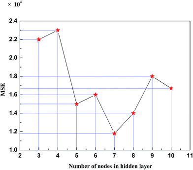
The model has selected two variables, temperature and pressure, as the input variables, and it will output the solubility predicted by the model. The amount of nodes in the hidden layer can be obtained by the trial-and-error method. 8 models will be respectively established assuming the number of nodes in the hidden layer from 3 to 10. Fig. 1 shows the variation of the MSE of the model with the changing amount of nodes in the hidden layer. It can be concluded that when there are 7 nodes in the hidden layer, the minimum model error appears.

Fig. 1 Results of topology studies for the optimal ANN configuration.

Thus, the CEAPSO KHM RBF ANN model of CO₂ solubility in polymers is developed, and the structure is 2-7-1. In Fig. 2 and 3 the prediction of CO₂ solubility in polymers by the CEAPSO KHM RBF ANN is plotted against the experimental values for the training and validation sets, in which the straight line indicates the perfect state where the predicted value equals the experimental value, and the vertical dimension between the predicted data point and the straight line presents the absolute deviation between the predicted value and the experimental value. As shown in these figures, the proposed model for the training set and validation set all have good predictive ability and the vertical dimension between the predicted data point and the straight line is relatively short; that is, the deviation between the predicted value and the experimental value is small.

Fig. 2 Predicted data versus experimental data in the training set.

Fig. 3 Predicted data versus experimental data in the validation set.

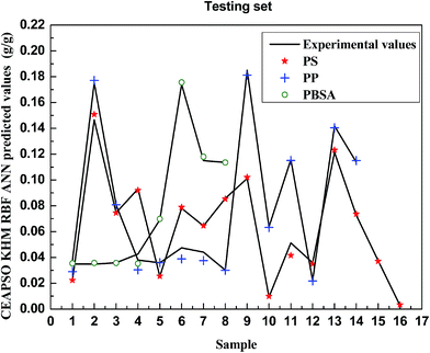
Fig. 4 and 5 plot the correlations between the predicted value and experimental value for the testing set. It can be seen from the figures that the difference between the calculated data and experimental data is very low and it is showing that the CEAPSO KHM RBF ANN model is a powerful tool for predicting CO₂ solubility in polymers. Especially, the model performs much better on PP, CPEs and PVAc; the predicated values are almost equal to the experimental values.

Fig. 4 Predicted data versus experimental data in testing set (1).

Fig. 5 Predicted data versus experimental data in testing set (2).

Table 2 gives the statistical data of prediction on various polymers in the testing set. The results show that the model can accurately predict the solubility of CO₂ in polymers, and the output of the model is relatively identical to the expectation. Table 2 also indicates that both the prediction accuracy and correlation of the model have performed well as a combination property.

Table 2 Values of ARD, R² and RMSEP in the testing set

Polymer	ARD	R^2	RMSEP
PVAc	0.1035	0.9959	0.0104
PS	0.1028	0.9978	0.0106
PP	0.1013	0.9987	0.0105
PBSA	0.1029	0.9984	0.0106
CPE55	0.0956	0.9991	0.0102
CPE60	0.0962	0.9987	0.0101
CPE67	0.0987	0.9985	0.0102
Average	0.1001	0.9982	0.0104

---

3.2 Comparative results

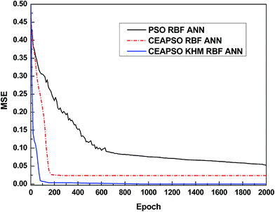
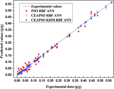
Firstly, two models of the same variety, the PSO RBF ANN and CEAPSO RBF ANN, are selected as comparative models in order to validate the combination property of these models. Comparison among these models is not an easy task because all of these models are based on the same data. In fact, a fair comparison is only achieved when all the models are constructed on the same data set. Thereupon, we randomly selected 10 data points from each polymer to get a database with 70 data points for the comparison. Fig. 6 shows the convergence curves of each model. It can be concluded from the figure that the convergence rate of each model is normal. The CEAPSO KHM RBF ANN model achieves stable convergence upon the 100^th iteration approximately, and the CEAPSO RBF ANN model also gradually becomes stable upon the 180^th iteration. However, in terms of the convergence precision, the model proposed in this work is better than the other models.

Fig. 6 Curve of the MSE vs. epoch.

Fig. 7 shows the comparison between the predicted solubility and experimental values of each model. As we can see from this figure, the distance between the predicated data point and the straight line of the model proposed in this work is small. It means that the predicated data points are mostly falling near the straight line, the predicated values are nearly identical to the experimental values, and the prediction error is relatively small. The figure shows that a good agreement is obtained with the CEAPSO KHM RBF ANN model while the performance of the CEAPSO RBF ANN and PSO RBF ANN are less satisfactory.

Fig. 7 Predicted data vs. experimental data in the testing database.

Moreover, several solubility prediction models proposed in recent years are selected as comparative models in order to show the advances and significance of the model in the current work, such as the CSPSO-C RBF ANN,³⁴ CSPSO-FC RBF ANN,³³ and CSPSO-KHM RBF ANN.³¹ Table 3 indicates the statistical data of these models.

Table 3 Statistical parameters of the comparison models

Model	ARD	R^2	RMSEP	Best fitness	Time (s)
Model proposed in ref. 34	0.1282	0.9970	—	5.96 × 10^−7	—
Model proposed in ref. 33	0.1071	0.9973	—	4.78 × 10^−7	16.79
Model proposed in ref. 31	0.1051	0.9975	0.0107	4.52 × 10^−7	21.76
Model proposed in this work	0.1001	0.9982	0.0103	3.67 × 10^−7	6.78

---

In terms of the accuracy and corrections, the CEAPSO KHM RBF ANN model proposed in this article is slightly better and has the lowest deviations compared with the other models. In terms of the convergence speed, the CEAPSO KHM RBF ANN model is faster, and it achieves stable convergence upon the 100^th iteration approximately, while the CSPSO-C RBF ANN,³⁴ CSPSO-FC RBF ANN³³ and CSPSO KHM RBF ANN³¹ need approximately 500, 380 and 300 iterations, respectively. Importantly, the calculation time is much shorter, at about one third of the others. The shorter calculation time is attributed to the training algorithm of the model, which adopts APSO with a rapid convergence speed.

Overall, we can see that both the convergence speed and corrections of the CEAPSO KHM RBF ANN model are superior to the others; the performance of the model in the current work is better and has obvious advantages in predication accuracy and correlation compared with that in the recently published articles.

3.3 Discussion and analysis

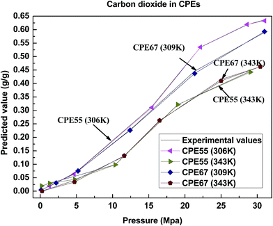
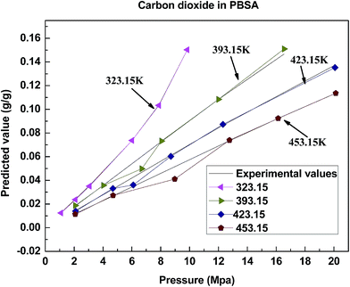
The results presented in this work show that the proposed model is reliable in predicting the solubility of gas in polymers, it has presented its good performance for solubility prediction, and achieves a satisfying effect in accuracy, execution time and correlation. It can be known from the comparison with other models that the combination property of the model in this article has significant advantages. The reasons for its excellent performance mainly contain two aspects. On one hand, the training algorithm of the model adopts APSO with a rapid convergence speed, and it also improves the problem of prematurity through chaotic disturbance; on the other hand, the KHM clustering method has made the model training more targeted and purposeful, and the center and spread of the radial basis function are more reasonable.

In many gas/polymer systems, the solubility increases almost linearly with pressure. Take 4 polymers as an example, consisting of PBSA, PP, PVAc and CPEs. Fig. 8–11 show the correlations between the predicted solubility and experimental data for CO₂/polymer systems at various pressures and temperatures.

Fig. 8 Correlations between predicted values and experimental data for CPEs.

Fig. 9 Correlations between predicted values and experimental data for PBSA.

Fig. 10 Correlations between predicted values and experimental data for PP.

Fig. 11 Correlations between predicted values and experimental data for PVAc.

These figures show that the solubility of CO₂ in most polymers increases with increasing pressure and decreasing temperature, and it is consistent with the tendency of the solubility experiment. This tendency can be explained by the plasticizing effect. The mobility increases with the increasing pressure because the molecules are forced between the polymer chains leading to the space expanding between molecules. Once the pressure is further raised, more gas molecules will be absorbed with an increased mobility of the chains. At the same time, the gas density descends with the increasing temperature, which can be correlated with the lower solubility.

4. Conclusions

In order to show the applicability of the proposed model for solubility prediction of carbon dioxide in polymers, a hybrid model called CEAPSO KHM RBF ANN was developed in this work. Through test and comparison, the model’s advancement has been proven, and a reliable prediction technique has been provided for research on solubility. The model in this article not only can be used in the field of prediction, but can also be expanded to wider applications and research fields, such as thermodynamics, self-assembly of high polymer materials, kinetic analysis and so forth, so as to analyze the chemical characteristics, physical characteristics, mechanical properties, rheological properties and other features of various materials. These results in this work should contribute to the enlargement of the database necessary for understanding the phase behaviour of the gas/polymer system, and for the design and optimization of processing techniques.

Abbreviations

RBF	Radial basis function
ANN	Artificial neural network
PSO	Particle swarm optimization
APSO	Accelerated particle swarm optimization
CEAPSO	Chaos-enhanced accelerated particle swarm optimization
KHM	K-harmonic means
PP	Polypropylene
PS	Polystyrene
PVAc	Poly(vinyl acetate)
CPEs	Carboxylated polyesters
PBSA	Poly(butylene succinate-co-adipate)
ARD	Average relative deviation
R^2	Squared correlation coefficient
MSE	Mean square error
RMSEP	Root mean square error of prediction

References

1. S. L. Liu, L. Shao, M. L. Chua, C. H. Lau, H. Wang and S. Quan, Prog. Polym. Sci., 2013, 38, 1089–1120.
2. X. Han and M. Poliakoff, Chem. Soc. Rev., 2012, 41, 1428–1436.
3. Q. Zhang, N. Vanparijs, B. Louage, B. G. de Geest and R. Hoogenboom, Polym. Chem., 2014, 5, 1140–1144.
4. Z. G. Lei, C. N. Dai and B. H. Chen, Chem. Rev., 2014, 114, 1289–1326.
5. M. Galizia, Z. P. Smith, G. C. Sarti, B. D. Freeman and D. R. Paul, J. Membr. Sci., 2015, 475, 110–121.
6. M. Fischlschweiger and S. Enders, Macromolecules, 2014, 47, 7625–7636.
7. L. Pogliani and J. V. de Julian-Ortiz, RSC Adv., 2013, 3, 14710–14721.
8. M. Minelli and M. G. de Angelis, Fluid Phase Equilib., 2014, 367, 173–181.
9. H. Ziaee, S. M. Hosseini, A. Sharafpoor, M. Fazavi, M. M. Ghiasi and A. Bahadori, J. Taiwan Inst. Chem. Eng., 2015, 46, 205–213.
10. R. Jalem, M. Nakayama and T. Kasuga, J. Mater. Chem. A, 2014, 2, 720–734.
11. Q. Wang, O. G. Apul, P. F. Xuan, F. Luo and T. Karanfil, RSC Adv., 2013, 3, 23924–23934.
12. J. S. Torrecilla, C. Tortuero, J. C. Cancilla and P. Diaz-Rodriguez, Talanta, 2013, 116, 122–126.
13. Y. Bakhbakhi, Math. Comput. Model., 2012, 55, 1932–1941.
14. H. Pahlavanzadeh, S. Nourani and M. Saber, J. Chem. Thermodyn., 2011, 43, 1775–1783.
15. B. Mehdizadeh and K. Movagharnejad, Fluid Phase Equilib., 2011, 303, 40–44.
16. F. Gharagheizi, A. Eslamimanesh, A. H. Mohammadi and D. Richon, Ind. Eng. Chem. Res., 2011, 50, 221–226.
17. A. Khajeh and H. Modarress, Expert Syst. Appl., 2010, 37, 3070–3074.
18. J. F. Pei, C. Z. Cai, Y. M. Zhu and B. Yan, Macromol. Theory Simul., 2013, 22, 52–60.
19. X. Zhao, M. C. Nguyen, C. Z. Wang and K. M. Ho, RSC Adv., 2013, 3, 22135–22139.
20. J. Luo, W. Lin, X. Cai and J. Li, Chin. J. Chem. Eng., 2012, 20, 950–957.
21. R. Pacheco-Contreras, D. J. Borbon-Gonzalez, M. Dessens-Felix, L. O. Paz-Borbon, R. L. Johnston, J. C. Schon, M. Jansen and A. Posada-Amarillas, RSC Adv., 2013, 3, 11571–11579.
22. L. Zhuo, J. Zhang, P. Dong, Y. D. Zhao and B. Peng, Neurocomputing, 2014, 134, 111–116.
23. Z. Beheshti and S. M. H. Shamsuddin, Inf. Sci., 2014, 258, 54–79.
24. T. T. Nguyen, Z. Y. Li, S. W. Zhang and T. K. Truong, Expert Syst. Appl., 2014, 41, 2134–2143.
25. S. E. K. Fateen and A. Bonilla-Petriciolet, Ind. Eng. Chem. Res., 2014, 53, 10826–10834.
26. X. W. Xia, J. N. Liu and Z. B. Hu, Appl. Soft Comput., 2014, 23, 76–90.
27. S. E. K. Fateen and A. Bonilla-Petriciolet, Fluid Phase Equilib., 2014, 375, 360–366.
28. X. G. Liu and C. Y. Zhao, AIChE J., 2012, 58, 1194–1202.
29. J. A. Lazzus, Fluid Phase Equilib., 2010, 289, 176–184.
30. M. S. Li, X. Y. Huang, H. S. Liu, B. X. Liu, Y. Wu, A. H. Xiong and T. W. Dong, Fluid Phase Equilib., 2013, 356, 11–17.
31. M. Li, X. Huang, H. Liu, B. Liu, Y. Wu and L. Wang, RSC Adv., 2015, 5, 45520–45527.
32. M. S. Li, X. Y. Huang, H. S. Liu, B. X. Liu, Y. Wu and F. R. Ai, Acta Chim. Sin., 2013, 71, 1053–1058.
33. Y. Wu, B. X. Liu, M. S. Li, K. Z. Tang and Y. B. Wu, Chin. J. Chem., 2013, 31, 1564–1572.
34. M. S. Li, X. Y. Huang, H. S. Liu, B. X. Liu and Y. Wu, J. Appl. Polym. Sci., 2013, 130, 3825–3832.
35. W. B. Wang, Q. Y. Feng and D. Liu, Prog. Electromagn. Res., 2011, 115, 173–189.
36. C. H. Yang, S. W. Tsai and L. Y. Chuang, Appl. Math. Comput., 2012, 219, 260–279.
37. A. H. Gandomi, G. J. Yun, X. S. Yang and S. Talatahari, Comm. Nonlinear Sci. Numer. Simulat., 2013, 18, 327–340.
38. F. Q. Yang, T. L. Sun and C. H. Zhang, Expert Syst. Appl., 2013, 40, 4735.
39. A. Khajeh, H. Modarress and M. Mohsen-Nia, Iran. Polym. J., 2007, 16, 759–768.
40. Y. Sato, K. Fujiwara, T. Takikawa, Sumarno, S. Takishima and H. Masuoka, Fluid Phase Equilib., 1999, 162, 261–276.
41. Z. G. Lei, H. Ohyabu, Y. Sato, H. Inomata and R. L. Smith, J. Supercrit. Fluids, 2007, 40, 452–461.
42. D. C. Li, T. Liu, L. Zhao and W. K. Yuan, Ind. Eng. Chem. Res., 2009, 48, 7117–7124.
43. Y. Sato, T. Takikawa, A. Sorakubo, S. Takishima, H. Masuoka and M. Imaizumi, Ind. Eng. Chem. Res., 2000, 39, 4813–4819.
44. Y. Sato, M. Yurugi, K. Fujiwara, S. Takishima and H. Masuoka, Fluid Phase Equilib., 1996, 125, 129–138.
45. S. Hilic, S. Boyer, A. Padua and J. Grolier, J. Polym. Sci., Part B: Polym. Phys., 2001, 39, 2063–2070.
46. Y. Sato, T. Takikawa, S. Takishima and H. Masuoka, J. Supercrit. Fluids, 2001, 19, 187–198.
47. M. Skerget, Z. Mandzuka, E. Aionicesei, Z. Knez, R. Jese, B. Znoj and P. Venturini, J. Supercrit. Fluids, 2010, 51, 306–311.
48. G. E. Tsekouras and J. Tsimikas, Fuzzy Sets Syst., 2013, 221, 65–89.
49. A. Alexandridis, E. Chondrodima and H. Sarimveis, IEEE Trans. Neural Netw. Learn. Syst., 2013, 24, 219–230.

---