Linear solvent structure-polymer solubility and solvation energy relationships to study conductive polymer/carbon nanotube composite solutions

Abstract

The solvation and solvent selectivity of polymer composites in different solvents is an important subject in colloid and polymer chemistry. Two multiparameter linear models based on theoretical and empirical parameters were constructed and validated for 59 and 54 solvents, respectively, to predict the relative energy difference (RED) of the solvents and a conductive polymer composite containing carbon nanotube. In addition to the excellent external prediction ability, models 1 (QSPR) and 2 (LSER) covered 87% and 93% of cross-validated variance, respectively. Different statistical methods were applied to test and validate the models. From the descriptive view, it was shown by model 1 that the compactness of solvent structure, mass and polar interactions are important in the resistance of the polymer and its RED in the desired solvent. In addition to the Hildebrand solubility parameter, acidity of the solvent and hydrogen bonding interactions have a direct relationship with RED. Both the models confirmed the moderate and complex effect of polar interactions in the solvation of desired polymer composites in different solvents.

---

1. Introduction

Electrically conductive polymer composites (CPCs) are a type of smart material, which have come into the focus of research because of their highly applicable characteristics. Smart materials are solid-state transducers that have different sensing and actuating properties like electroactivity, piezoelectric electrostrictivity, pyroelectricity, magnetostrictivity and piezoresistivity.¹ The most promising and viable strategy for the successful development of electrically conductive polymer composites (CPCs) is the blending of a customary polymer with electrically conductive fillers.

The exceptional intrinsic properties of carbon nanotubes (CNTs), such as thermal and electrical conductivity or mechanical properties, has made them one of the most promising nanomaterials that are used to modify the properties of polymer and conductive polymer composites.² Moreover, CNTs have high length/diameter ratios (aspect ratios) of about 100–1000, which leads to moderately low percolation thresholds in composite materials in comparison with carbon fiber or carbon black.³ Conductive polymer/nanofiller composites have been widely investigated in industry and academia because of their outstanding multifunctional properties compared to conventional conductive polymer composites (CPCs). Polymer/carbon nanofiller composites can be used for electrostatic dissipation (ESD),⁴ electromagnetic interference-shielding (EMI-shielding),^1,5,6 electrostatic painting,⁷ and mechanical reinforcement.^8,9 Some of the important aspects of CPCs are their relative resistance change and solvent selectivity as a key property of these sensory polymers.¹⁰

Few reports have been published on the establishment of correlations between relative resistance changes of CPCs and solvents' solubility parameters. Chen et al. reported that waterborne polyurethane composites filled with carbon black show a maximum relative resistance change that correlates with the polar component of Hansen solubility (δ_P).¹¹ Fan et al. found the same result for thermoplastic polyurethane multifilament covered with carbon nanotube networks.¹² A study on the role of difference of the solubility parameters between polymer matrix and tested solvents (Δδ) in polystyrene/carbon black composites were also done by Li et al.¹³ The Flory–Huggins interaction parameter, χ₁₂, was also utilized to correlate relative resistance change of CPCs/CNTs against some solvent vapors;^14,15 however, this approach is almost not sufficiently accurate.¹⁶ Villmow et al. investigated the relative resistance change of a CPC with 1.5 wt% CNT immersed in different organic solvents and calculated the Hansen solubility parameters of the CPC.¹⁶ They also described the selectivity of the CPC by using two parameters, namely, the distance in Hansen space R_a and the solvents' molar volume V_mol.

In the current study, we focused on CPCs based on polycarbonate (PC) filled with 1.5 wt% carbon nanotubes¹⁶ in different solvents in order to scrutinize the details of the interactions between solvent and CPCs and the role of solvent characteristics in the dispersibility of the CPCs and their solvent selectivities. We used quantitative structure property relationship (QSPR) and linear solvation energy relationship (LSER), one of the well-known approaches of QSPR, to predict the relative energy difference (RED) of CPC/CNT and different solvents. In the proposed approach for the first time, some solvent empirical parameters were utilized to clear solvent–polymer interactions and for prediction purposes. Herein, we tried to emphasize the role of solvent in solvent-sensory polymers using a predictive and descriptive method.

2. Materials and methods

2.1. Data set preparation and processing

In this study, two types of models were used for the examination of the dispersibility of PC/CNT composite in different solvents. In the first model, the theoretical and structural descriptors of solvents were used to construct a QSPR model to predict the RED numbers of PC/CNT composite in 59 solvents adapted from literature.¹⁶ RED number of 0 is found for no energy difference. RED numbers less than 1.0 indicate high affinity; RED equal to or close to 1.0 is a boundary condition; and progressively higher RED numbers indicate lower affinities.¹⁷ The name of the solvents and their RED values are presented in Table 1. In the first step, the chemical structures of these 59 solvents were drawn in Hyperchem software (Version 7, Hypercube Inc., http://www.hyper.com, USA) and optimized using the semi-empirical method of AM1. Then, molecular descriptors were calculated for desired solvents from the optimized chemical structures by Dragon software (Milano Chemometrics and QSAR research group; http://michem.disat.unimib.it/chm/). Furthermore, it was crucially important to do several complementary works. In other words, numerous molecular descriptors were lessened by removing descriptors that could not be calculated for every structure in the dataset and those descriptors with an essentially constant or near constant value for all structures. In addition, to decrease the redundancy in the descriptors data matrix, the correlations among X-variables and with the RED vector were examined, and among the detected collinear variables (i.e., R² > 0.95), the one with the highest correlation with RED was retained and the others were removed from the data matrix. After these steps, 834 descriptors remained for each solvent.

Table 1 Experimental and predicted RED number of PC/CNT composite in various solvents

No.	Solvent	RED (exp.)	RED (pred1)^a	RED (pred2)^b
a The predicted values using model 1, eqn (1).b The predicted values using model 2, eqn (2).c Compounds in the test set using model 1.d Compounds in the test set using model 2.
1	Acetophenone	0.18	0.32	0.33
2^c	Cyclohexanone	0.26	0.42	0.44
3^d	n-Methyl-2-pyrrolidone	0.31	0.42	0.39
4^c	Ethylene dichloride	0.32	0.36	0.51
5	Isophorone	0.37	0.60	—
6^c	2-Nitropropane	0.40	0.46	0.55
7	o-Dichlorobenzene	0.44	0.38	0.44
8	Methyl ethyl ketone	0.47	0.63	0.50
9	Methylene dichloride	0.48	0.57	0.54
10	Mesityl oxide	0.49	0.67	—
11^d	Diethyl ketone	0.55	0.72	0.57
12^d	Butyronitrile	0.57	0.62	0.64
13^d	Acetone	0.58	0.84	0.55
14	Nitroethane	0.59	0.67	0.69
15	Chlorobenzene	0.62	0.41	0.61
16^c	Anisole	0.64	0.56	0.62
17^d	Tetrahydrofuran	0.64	0.62	0.67
18	Methyl acetate	0.68	0.72	0.69
19	Propylene carbonate	0.69	0.54	0.63
20	Acetic anhydride	0.69	0.58	0.58
21	Methyl butyl ketone	0.69	0.67	0.47
22	Methyl isobutyl ketone	0.69	0.76	0.50
23	Trichloroethylene	0.70	0.70	0.59
24^d	Dimethylformamide	0.71	0.73	0.61
25^d	Chloroform	0.71	0.80	0.70
26^c	Diethyl carbonate	0.71	0.98	0.72
27	Dimethyl sulfoxide	0.73	0.50	0.60
28^c	Ethyl acetate	0.73	0.66	0.70
29	Di-(2-methoxyethyl) ether	0.77	0.83	0.64
30	Diethylene glycol monobutyl ether	0.79	0.74	—
31	n-Butyl acetate	0.81	0.69	0.68
32	Morpholine	0.81	0.95	0.95
33	Aniline	0.83	1.21	0.72
34	Furan	0.85	0.84	1.06
35^c	Nitromethane	0.86	0.93	0.76
36	Toluene	0.86	0.72	0.87
37^c	Diethylene glycol monomethyl ether	0.89	0.83	—
38	Ethylene glycol monoethyl ether acetate	0.91	0.69	—
39	Isoamyl acetate	0.92	0.70	0.72
40	1,4-Dioxane	0.93	0.81	0.92
41^c	m-Cresol	0.93	0.75	1.01
42	Ethyl benzene	0.95	0.89	0.88
43	Mesitylene	0.97	0.87	0.98
44^d	Benzene	0.98	0.80	0.89
45	Diethyl ether	0.99	0.93	1.01
46^c	Dipropyl amine	1.00	1.14	1.00
47	Cyclohexanol	1.04	1.06	1.31
48^c	Cyclohexane	1.06	1.07	1.12
49^d	Ethylene glycol monomethyl ether	1.08	1.09	1.17
50	n-Hexane	1.20	1.50	1.12
51	1-Butanol	1.21	1.11	1.30
52	Diethylene glycol	1.36	1.17	1.40
53^d	Ethanol	1.44	1.52	1.48
54^c^,^d	Propylene glycol	1.55	1.29	1.57
55	Ethanolamine	1.57	1.70	1.47
56^d	Methanol	1.74	1.82	1.63
57^c	Formamide	1.90	1.80	1.93
58	Ethylene glycol	1.95	1.53	2.10
59	Water	3.45	3.34	3.26

---

In the second model based on empirical solvent scales, 127 scales of three principal classes (equilibrium-kinetic, spectroscopic and multiparameters of other measurements)¹⁸ were used for LSER modeling of the RED of polymer–solvents. Among the 59 solvents used in the previous model, the experimental parameters of 54 solvents were available and were used for model construction and validation. Moreover, the correlation between solvent scales was checked to delete the redundant parameters.

2.2. Data modeling

The main goal of QSPR is to establish a significant relation based on few structure-based molecular descriptors, which can accurately predict an experimental property/activity (here RED of polymer/solvent samples). As it is feasible to produce a great number of molecular descriptors for each solvent in the dataset, a thorny problem is the selection of the set of molecular descriptors in order to build an accurate relationship. In the presented study, multiple linear regression analysis (MLR) with stepwise selection of variables (using SPSS software, SPSS Inc., version 15.0) was applied to relate the solvent structural parameters with the solubility of PC/CNT composite.

In order to get a better performance, all selected independent and dependent variables, theoretical descriptors/empirical solvent scales and RED vector were auto scaled. For model evaluation, the data of both models (QSPR and LSER) were divided into two parts: a training set for model building and a test set for checking the model's predictability. Cross validation and y-scrambling were also done to test the stability and significance of models.

All calculations were run on a laptop computer under the Windows XP operating system. MATLAB (version 7, Math work, Inc., http://mathworks.com, USA) was used for the MLR analysis and other statistical calculations.

3. Results and discussion

3.1. Model construction based on structural parameters of solvents (model 1)

The study was conducted based on 834 solvent structural parameters for 59 solvents with known RED numbers for a PC/CNT composite.¹⁶ Hence, a data matrix with the size of 59 × 834 was achieved. Randomly, 13 solvents out of 59 (about 20%) were chosen as test samples, while the remaining 46 solvents (about 80%) were utilized as the training set. It can be noted that the RED numbers of solvents in the training set covered the RED number of the whole data set. The range from 0.18 to 3.45 of RED numbers was selected for the training set and the values of the test set were in the range from 0.26 to 1.90. It is clear that the concept of RED in the PC/CNT composite material is similar to the concept in regular polymers.

Seven different models were created step-by-step through a stepwise regression run but some of them may be over fitted. A cross-validation method was applied for each model so that the most convenient correlation equation was selected. The plots of variation of the calibration-squared correlation coefficient (R_cal²) and cross validation (Q²) are illustrated in Fig. 1a. As can be seen, the model performance was refined by up to four variables by introducing each new variable and after that no drastic change was observed. The resultant four-parametric equation is as follows:

RED = 0.895(±0.024) − 0.283(±0.025)FDI + 0.236(±0.30)GATS1e − 0.148(±0.033)BEHe8 + 0.106(±0.034)RDF010m (1)

N = 59, N_train = 46, N_test = 13, R_train² = 0.91, Q_LOO² = 0.87, F = 102.58, F_crit. = 2.60

In this equation, FDI is related to the folding degree index, GATS1e is the Geary autocorrelation coefficient lag1, which is weighted by atomic Sanderson electronegativities, BEHe8 shows the highest eigenvalue (number 8) of the Burden matrix weighted by atomic Sanderson electronegativities and RDF010m is a radial distribution function descriptor weighted by atomic Sanderson electronegativities and atomic masses, respectively (Table 2). With the relative amounts of contribution of each of these parameters, it is possible to estimate relevant information about the solvent–PC/CNT composite interactions in the solution phase and will be discussed more in the next parts of the manuscript.

Fig. 1 The plot of model performance vs. number of variables included in model 1 (a) and plot of predicted RED numbers using the model 1 versus experimental values (b).

Table 2 The brief definitions of variables of the proposed models

Solvent scale	Definition	Property of scale
FDI	Folding degree index	Molecular size and volume
GATS1e	Geary autocorrelation coefficient lag1/weighted by atomic Sanderson electronegativities	Topology and electronegativity/polarity
BEHe8	Highest eigenvalue no. 8 of Burden matrix/weighted by atomic Sanderson electronegativities	Topology and electronegativity/polarity
RDF010m	Radial distribution function-1.0/weighted by atomic masses	Topology and structural mass
Ap	Acidity parameter calculated from the data for the Gibbs solvation energy for the alkali metal cations and halide ions	Acidity
SPP^N	Calculated from the UV-Vis spectra of 2-(dimethyl-amino)-7-nitrofluorene and its homomorph 2-fluoro-7-nitrofluorene	Dipolarity and dipolarizability
δ^H	Square root of cohesive energy density	Total cohesive energy density
X^Re	Selectivity parameter: reflects a composite of solvent dipolarity–dipolarizability, hydrogen bond acidity and hydrogen bond basicity	Dipolarity–dipolarizability and hydrogen bonding

---

Moreover, N is the number of the solvent, R_train² is the squared correlation coefficient of calibration (training set) and Q_LOO² is the squared correlation coefficients for leave-one-out cross-validation and their values show the goodness and stability of the proposed model. F is the Fischer F-statistic and F_crit. is the F-critical value. The high value of calculated F (in comparison with F_crit.) verified the statistical significance of the resultant model. Moreover, the values in parentheses are the coefficients' standard deviation and their low values indicate the significance of the selected parameters. In addition, the t-test showed the significance of the model with p-values almost equal to zero (Table S1, ESI†). It can be noted that this equation explained more than 91% of the variances in the PC/CNT composite solubility data with an excellent statistical quality.

After auto scaling of the selected parameters, the obtained standardized MLR-coefficients were used to calculate the values of RED number for the training and test sets and the predicted REDs are shown in Table 1. To check the stability of the proposed model, leave-one-out and leave-two out cross validations were also done and the squared correlation coefficients for cross-validation (Q_LOO² and Q_L2O²) were found to be 0.87 and 0.86, respectively. These parameters were indicators of model stability and prediction ability.

Furthermore, it has been proposed that the true predictive power of a QSPR model should be evaluated by an external test set of compounds that were not used in the model construction.¹⁹ Hence, the squared correlation coefficient (R_test²) and root mean square error of the test set (RMSEP) were calculated for further checking. It can be noted that the R_test² and RMSEP obtained were 0.91 and 0.31 respectively, which are another evidence of the excellent predictability of the obtained QSPR model. For better visualization, the predicted values were plotted versus the experimental values of the model in Fig. 1b. This figure displayed an outstanding agreement between experimental and predicted values of RED based on the proposed model.

Model validation is by far the most crucial step of QSPR and a great number of procedures have been generated for the determination of the quality of a QSPR model.²⁰ As it was explained, cross-validation and external validation procedures were established in this study for this goal. As a general rule of thumb, some statistical parameters, including the cross-validation square correlation coefficient (Q_cv²), prediction residual sum of squares and root mean square error in cross-validation (RMSEcv) are the most powerful parameters to check the cross-validation predictability.²¹ In comparison with R_cal², which can be improved by adding more parameters, Q_cv² declined in the presence of an over parameterized model.²² Therefore, the Q_cv² value is far more meaningful for measuring the average predictive power of a model and also it can be considered in order to select the optimum number of parameters (four-parametric linear model in this study).

The permutation test known as y-randomization or y-scrambling (randomization of response, i.e., RED in this study) is another procedure for checking the significance of the Q_cv² value.²³ In the current study, RED in the training set was scrambled 50 times and as the statistic parameter of the permutation test, a maximum of the cross-validated squared correlation coefficient of the scrambled data (Q_MS²) was calculated, which was 0.32 and far from the Q_cv² of the original model. This parameter could confirm that model 1 was not obtained by chance.

3.2. Model construction based on an empirical solvent scale

The empirical parameters for 54 out of 59 solvents were available in the literature and the data for 5 solvents (isophorone, mesityl oxide, diethylene glycol monobutyl ether, diethylene glycol monoethyl ether acetate and ethylene glycol monoethyl ether acetate) were not found. Therefore, this model was constructed based on the solvent empirical parameters of 54 solvents and after deleting the collinear variables, a data matrix with the size of 54 × 121 was obtained.

42 solvents were selected randomly for the training set, whereas 12 solvents were dedicated to the test set. As mentioned earlier, the RED number of the training set covered the RED number of the whole data set.

Again, stepwise MLR was employed for selecting the most relevant subset of scales among the solvent scales as independent variables. Similar to what was noted for QSPR model, cross validation were used to select the final model without the risk of over fitting. According to Fig. 2a, the performance of the model was not significantly improved after including 4 parameters. Thus, a four-parametric equation was selected:

RED = −0.360(±0.182) + 0.062(±0.007)Ap − 1.697(±0.199)SPP^N + 0.031(±0.006)δ + 0.751(±0.239)X^R_e (2)

N = 54, N_train = 42, N_test = 12, R_train² = 0.95, Q_LOO² = 0.93, F = 180.744, F_crit. = 2.6261

Fig. 2 The plot of model performance vs. number of variables included in model 2 (a) and plot of predicted RED number using the model 2 versus experimental values (b).

Because of the choice to use the solvent empirical parameters as independent variables of the model, this model could be considered as a linear solvation energy relationship (LSER). In the LSER approach, the effects of solvent–solute interactions on physicochemical properties and reactivity parameters are studied.²⁴ Our equation is similar to the LSERs, which have been proposed by Kamlet and Taft.^25,26

This model confirmed an acceptable relationship between the selected variables and the RED number of the solvents, which explained 95% of data variance. It can be noted that the model is statistically significant based on the F-statistics and t-test (see Table S2, ESI†). Moreover, the model represented cross-validation statistics similar to the calibration set. The high value of correlation coefficient of leave-one-out and leave-two-out cross validation for the LSER model (Q_LOO² = Q_L2O² = 0.93) and acceptable value of cross validation root mean square error (RMSE_cv = 0.27) proved the predictive power and the stability of the model based on the interstice error in experimental RED data (Table 1).

The root mean square error and correlation coefficient of the test set (RMSE_test and R_test²) were 0.15 and 0.98, respectively, which confirmed the high external predictive ability of the model. The y-randomization test also showed that this model was not a chancy model (Q_MP² = 0.29 compared to Q_cv² of original model = 0.93). Fig. 2b displays the predicted values versus the experimental values of the model, which illustrates an outstanding agreement between experimental and predicted values of RED.

3.3. Applicability domain

To show the scope and limitation of a QSAR model, the applicability domain (AD) is widely utilized. The concept for the applicability domain of a model is closely pertained to the term model validation. AD is defined as the substantiation that a model possesses a satisfactory range of accuracy within the intended application of the model.²⁷

The leverage of a compound produces a check for multivariate normality of observation.²⁸ In other words, it provides a measure of the distance of the compound from the centroid of the model space and the model building; moreover, the chemical compounds close to the centroid are less influential and beneficial. The so-called influence matrix or hat matrix (H) is given by:

H = X(X^TX)⁻¹X^T (3)

where X is the descriptor matrix, which is derived from the training set, X^T is the transpose of X and (X^TX)⁻¹ is the inverse of matrix (X^TX). The leverage or hat values (h_i) of the i^th compound in the descriptor space are the diagonal elements of H, which can be calculated by:

h_i = x_i(X^TX)⁻¹x^T_i (4)

where x_i is the descriptor row vector of the interest compound. h* or the warning leverage is defined as h* = 3m/n, where n is the number of training compounds and m is the number of model parameters plus one²⁸ (here 4 + 1 in both models 1 and 2). A compound that possesses a high leverage (bigger than a warning value) in the training set enjoys a remarkable influence on the regression line and can force the fitted line to be close to the observed value for that compound. The leverage values for all polymer/solvent samples in training and test sets were calculated for both models.

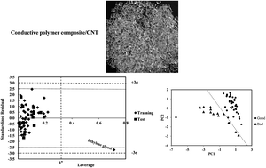
In addition to the high leverage values, it should be noted that some compounds may also be outside the AD due to their large standardized residuals.²⁸ As a result, Williams plots of the models can be utilized to identify the compounds outside the applicability domain,²⁴ which are shown in Fig. 3a and b for QSPR and LSER models, respectively. In this plot, both leverage and standardized residuals are taken into consideration to visualize the applicability domain. It is crystal clear that all solvents are in the applicability domain except water in model 2 and ethylene glycol in model 1 and 2, and most of the solvents have a standardized residual in the acceptable range of ±3σ.

Fig. 3 Williams plot of the entire set of solvents in model 1 (a) and model 2 (b). Cut off values of leverage (h*) and standardized residuals (±3 times the standards deviation) are depicted by vertical and horizontal dashed lines, respectively. Ethylene glycol is out of the applicable domain in model 1; ethylene glycol and water are out of the applicable domain in model 2.

3.4. Interpretation of models

Simplicity of use and interpretability are considered to be the outstanding merits of MLR. In addition, in modeling the target property (RED number), the magnitudes of coefficients show the relative significance of the descriptors and their signs indicate the positive or negative contribution of the molecular descriptors to the RED. It can be noted that the molecular descriptors should be mathematically independent of or orthogonal to each other and collinear descriptors can cause coefficients larger than expected or produce the wrong signs.²⁰

As it is shown in Table 3, which contains the correlation matrix of variables for both the models, the correlation coefficients amongst parameters are insignificant and negligible. The correlation matrix shows the inter-correlations between parameters of each model (QSPR and LSER). To check the multicollinearity of the parameters in each models, the variance inflation factor (VIF) was calculated for each variable²⁹ and is shown in the last column of Table 3.

Table 3 Correlation coefficients between parameters of QSPR and LSER models and their VIF values

	FDI	GATS1e	BEHe8	RDF010m	Ap	SPP^N	δ^H	X^Re	VIF^a
a Variation inflation factor.
FDI	1.000								1.202
GATS1e	0.094	1.000							1.358
BEHe8	0.065	0.000	1.000						1.830
RDF010m	0.002	0.141	0.348	1.000					1.995
Ap					1.000				3.654
SPP^N					0.006	1.000			1.245
δ^H					0.492	0.137	1.000		2.773
X^Re					0.386	0.001	0.197	1.000	2.000

---

If R_j² is the multiple correlation coefficient of one variable's effect regressed on the remaining molecular variables, the VIF of each theoretical descriptor in model 1 and each solvent empirical parameter in model 2 can be calculated according to the following equation:

It has been suggested that 5.0 is the cut-off value for VIF and if VIF would be larger than the cut-off value, the main information of descriptors can be concealed by the correlation of the descriptors.²⁹ According to Table 3, the VIF values of four parameters of the two models were less than 5.0. Therefore, the correlation matrix and VIF of parameters show that the statistical significance of the proposed models is acceptable and the sign and attribute of the coefficients could be used to describe the models.

3.4.1. Description of model 1. Standardized regression coefficients can be applied for the assessment of the relative importance of the variables included in an MLR model. The order of significance of the variables of eqn (1) is FDI > GATS1e > BEHe8 > RDF010m, which is shown in Fig. S1-a (ESI†). As it can be seen, the most significant parameter is FDI, while RDF010m is the less important variable of the model in the dispersibility of PC/CNT composite. FDI is the “folding degree index”, which is more applicable for peptides and proteins,³⁰ but is also used as a structural descriptor for other small molecules.³¹ Molecules with more folded structures (e.g. lower structural volumes) have higher FDI values. The negative sign of the MLR coefficient related to FDI in the proposed model shows that solvents with more unfolded structures and higher structural volume (lower FID) resulted in higher RED for PC/CNT. It can be noted that better solvents for PC/CNT have lower RED. This finding was in accordance with literature.¹⁶

The next two descriptors in the model GATS1e and BEHe8, “Geary autocorrelation coefficient lag1” and “Highest eigenvalue number 8 of Burden matrix”, respectively, and both of them are weighted with atomic Sanderson electronegativity.³¹ Therefore, it can be concluded that the electronegativity of solvents and consequently polar interactions have a significant role in solvation or dispersibility of PC/CNT. In addition, the positive sign of GATS1e and negative sign of BEHe8 imply that polar interactions may have an optimum value (not high, not low) for decreasing the RED.

The last parameter of the model was RDF010m, which is a radial distribution function weighted by atomic masses with a positive coefficient.³¹ It shows that the solvents with lower atomic mass possess lower RED and could be better solvents for PC/CNT.

3.4.2. Description of model 2. According to the standardized regression coefficient of model 2 and as it is illustrated in Fig. S1-b (ESI†), the order of importance of the variables of eqn (2) is Ap > SPP^N > δ^H > X^R_e.

Ap is the “acidity parameter” calculated from the data for the Gibbs solvation energy for the alkali metal cations and halide ions.³² According to the thermodynamic studies of the properties of electrolyte solutions, it is well-known that acidity and basicity are important in determining the properties of the solutions. The positive sign of Ap in eqn (2) shows the direct relationship of the acidity parameter of solvents and RED related to PC/CNT. So the good solvents, with lower RED, have lower acidity parameters.

SPP^N is a solvent empirical parameter calculated from the UV-Vis spectra of 2-(dimethyl-amino)-7-nitrofluorene and its homomorph 2-fluoro-7-nitrofluorene.³³ SPP^N is a solvent dipolarity–polarizability scale that combines medium dipolarity and polarizability into a single parameter. This scale is potentially useful for assessing the polarity of solution medium, and thus it can be assumed as an indicator of polar interactions. The negative sign of SPP^N in the proposed model shows that increasing the solvent polarity and polar interaction cause decrease in the RED of solvents and increasing solvation of PC/CNT.

The 3^rd parameter in the proposed model was δ, which is the squared root of cohesive energy density and is known as total solubility or Hildebrand solubility parameter.^17,34 According to the positive contribution of this parameter in the model (eqn (2)), decreasing the squared root of cohesive energy leads to decrease in the RED of a solvent. It should be emphasized that the values of δ (used for model construction) were adapted from the work of Katritzky et al.,¹⁸ in which the δ of some solvents have been measured experimentally and some others have been calculated computationally (based on experimental results). The well-known routine way to calculate the RED values of solvent–polymer systems is using Hansen solubility parameters. The basic equation to define Hansen parameters assumes that the total cohesion energy, E, has three parts:¹⁷

E = E_D + E_P + E_H (6)

The square of the total (or Hildebrand) solubility could be obtained by dividing this by the molar volume to give the parameter as the sum of the squares of the Hansen D, P, and H components (dispersive, polar and hydrogen bonding):

E/V = E_D/V + E_P/V + E_H/V (7)

δ² = δ_D² + δ_P² + δ_H² (8)

The interpretation of similarity between the two materials (indices 1 and 2) is possible by calculating their solubility parameter “distance” R_a based on their respective partial solubility parameters:¹⁷

R_a² = 4(δ_D1 − δ_D2)² + (δ_P1 − δ_P2)² + (δ_H1 − δ_H2)² (9)

A convenient single parameter to characterize solvent quality in this model is the relative energy difference, RED number:

RED = R_a/R_o (10)

where R_o is the interaction radius and R_a is the solubility parameter distance.

In this study, we showed that some other parameters could be important in the prediction and description of RED values in addition to the dependency of RED of solvent–PC/CNT to the cohesive energy components.

The last parameter of the proposed LSER model is X^R_e, which has a positive effect on RED. This parameter is defined as the selectivity parameter; it reflects a composite of a solvent's dipolarity–dipolarizability, hydrogen bond acidity and hydrogen bond basicity.³⁵ According to the discussion about SPP^N, it could be concluded that dipolarity–dipolarizability has a moderate effect on RED but hydrogen bonding interactions shows positive effects on RED. The results about the moderate effect of polar interaction were in agreement with model 1. In conclusion, better solvents for the solvation of PC/CNT might have lower hydrogen bonding interactions.

3.5. Comparison of the QSPR and LSER models

All statistical data of QSPR and LSER models are gathered in Table 4. The non-significant values of Q_cv² of the permutation test (Q_MP²) confirm that the models are reasonable and they are not obtained by chance. More importantly, although both proposed models resulted in very good statistics, LSER provides better statistical data for both calibration and prediction sets. Hence, the experimental solvent scale supplies remarkable ability to relate the dispersibility of PC/CNT composite with solvent type. In the LSER approach, the effects of solvent–solute interactions on physiochemical properties and reactivity parameters could be studied. However, a crucially important constraint of solvent scale is that they are experimental parameters and it is difficult to gather these data for new solvents. As a matter of fact, the application of the model is in need of previous experiments to measure the solvent scale. For instance, in our study, we could not find the solvent scales of five solvents. Another great advantage of solvent empirical parameters, in comparison with solvent theoretical descriptors, is their lower initial population, which decreases the risk of obtaining a chancy model in the case of limited number of compounds available for modeling.^36–38 While the descriptors of the QSPR model are calculated theoretically with the contribution of the available software and this model can be applied for the prediction of dispersibility in new solvents, even for virtual solvents that have not been synthesized or checked experimentally yet.

Table 4 Various statistics parameters of the developed model

	nv^a	Ntrain^b	Ntest^c	Rtrain^2^d	RMSEtrain^e	RLOO cv^2^f	RL2O cv^2^f	RMSEcv^g	Rtest^2^h	RMSEtest^i	QMP^2^j
a Number of descriptors applied for the model development.b Number of molecules in training set.c Number of molecules in test set.d Training correlation coefficient.e Training root mean square error.f Leave-one-out and leave-two-out cross-validation correlation coefficient.g Leave-one-out cross-validation root-mean-square errors.h Correlation coefficient of the test set.i Test root-mean-square errors.j Maximum cross-validation correlation coefficient for the y-randomization test.
Model 1 (QSPR)	4	46	13	0.91	0.30	0.87	0.86	0.36	0.91	0.31	0.32
Model 2 (LSER)	4	42	12	0.95	0.22	0.93	0.93	0.27	0.98	0.15	0.29

---

3.6. Exploratory data analysis

Because of the success of proposed models to predict the RED of polymer/solvents, principal component analysis (PCA) was utilized on the parameters of each model (1 and 2) for an exploratory data analysis of relative resistance change (R_rel) of PC/CNT in the different discussed solvents. R_rel could be calculated using the time dependent resistance, R(t), of the samples over immersion time in solvent and initial resistance, R_i, according to the following equation:

Information about the sensory composite's response to the solvent contact (good: R_rel > 0 or bad: R_rel ∼ 0) was adapted from the work of Villmow et al.¹⁶ and is represented in Table S3 (ESI†).

2D-plot of PC1 vs. PC2 of the parameters of model 1 based on the theoretical descriptors and model 2 constructed from empirical scales are shown in Fig. 4a and b, respectively. As it is clear from Fig. 4, both set of used parameters shows acceptable discrimination between good and bad solvents and can be an indicator of solvent selectivity.

Fig. 4 Discrimination of “good” and “bad” solvents for PC/CNT using principal component analysis on parameters entered in model 1 (a) and model 2 (b).

3.7. Test on another kind of polymer

To show the generality of the proposed model, the utilized parameters in model 1 and model 2 were used to check the behavior of another type of a polymer. The original RED data used above for the construction of models belonged to a polymer composite based on PC Lexan 141R (SABIC Innovative Plastics).¹⁶ We used another data set based on a R polycarbonate polymer.¹⁷ The RED of this polymer in the same solvents noted for PC Lexan 141R were used as the dependent variable for the model construction base on the parameters in two proposed model (eqn (1) and (2)). The RED values of this polymer in the discussed 59 solvents are represented in Table S4 (ESI†). Furthermore, similar to what was done for the original data, RED data of R polycarbonate polymer was divided into two parts: training and test sets. It was observed that both series of parameters used in model 1 and model 2 show good ability in the prediction of RED of the new type of polymer. This ability was checked using different statistical parameters related to training, cross validation and the test set that is presented in Table 5. The agreement between predicted RED and their experimental values are also shown graphically in Fig. 5. The MLR coefficient of the models for this R polycarbonate polymer using the parameters of model 1 and model 2 and Williams plots of these two new models are represented in ESI (Tables S5, S6 and Fig. S2†). The results show the ability of the proposed models to predict the behavior of other types of similar polymers.

Table 5 Various statistics parameters of the developed model for RED of the R polycarbonate polymer to show the applicability of proposed model for other type of polymers

	nv^a	Ntrain^b	Ntest^c	Rtrain^2^d	RMSEtrain^e	RLOO cv^2^f	RL2O cv^2^f	RMSEcv^g	Rtest^2^h	RMSEtest^i	QMP^2^j
a Number of descriptors applied for the model development.b Number of molecules in training set.c Number of molecules in test set.d Training correlation coefficient.e Training root mean square error.f Leave-one-out and leave-two-out cross-validation correlation coefficient.g Leave-one-out cross-validation root-mean-square errors.h Correlation coefficient of the test set.i Test root-mean-square errors.j Maximum cross-validation correlation coefficient for the y-randomization test.
Model 1 (QSPR)	4	46	13	0.91	0.30	0.88	0.87	0.35	0.94	0.25	0.35
Model 2 (LSER)	4	42	12	0.94	0.25	0.90	0.91	0.32	0.97	0.18	0.33

---

Fig. 5 Plot of predicted RED number using the parameters in model 1 (a) and in model 2 (b) versus experimental values.

4. Conclusion

New approaches were proposed based on QSPR and also a type of LSER to predict RED of solvents–PC/CNT and the validity, stability and prediction ability of the models were verified using different statistical methods. It was shown that the conductive polymer composites/carbon nanotube has better selectivity (lower RED) in solvents with more folded molecular structures (lower structural volume) and lower structural mass. According to both the positive and negative effects of structural electronegativity on RED, it was concluded that polar interactions have a moderate effect on the solvation of the desired PC/CNT.

Some other aspects of solvent–PC/CNT interactions also emerged using the 4 parametric LSER model. The suggested model showed that in addition to the total (or Hildebrand) solubility parameter, the acidity parameter of solvent and hydrogen bonding interactions have direct relationship with RED. However, polarity–polarizability interactions show two-side (reverse and direct) effects on the RED and selectivity. Therefore, the role of this type of interaction in our polymer–solvent system is more complex.

The combination of using theoretical descriptors and solvent empirical parameters resulted in a successful experience in the investigation of solvation of PC/CNT in different organic solvents.

Extension of this study on conductive polymer composites with different amounts of CNTs is in progress of our future research.

Acknowledgements

Support of Iran National Science Foundation (INSF) is gratefully acknowledged.

References

1. H. M. Kim, K. Kim, C. Y. Lee, J. Joo, S. J. Cho, H. S. Yoon, D. A. Pejaković, J. W. Yoo and A. J. Epstein, Appl. Phys. Lett., 2004, 84, 589.
2. P. Pötschke, A. R. Bhattacharyya and A. Janke, Carbon, 2004, 42, 965–969.
3. B. Krause, T. Villmow, R. Boldt, M. Mende, G. Petzold and P. Pötschke, Compos. Sci. Technol., 2011, 71, 1145–1153.
4. F. H. Ferguson DW, Bryant EWS, in SPE/ANTEC '98 Proceedings, 1998, pp. 1219–1222.
5. C.-C. M. Ma, Y.-L. Huang, H.-C. Kuan and Y.-S. Chiu, J. Polym. Sci., Part B: Polym. Phys., 2005, 43, 345–358.
6. Y. Yang, M. C. Gupta, K. L. Dudley and R. W. Lawrence, J. Nanosci. Nanotechnol., 2005, 5, 927–931.
7. O. Breuer and U. Sundararaj, Polym. Compos., 2004, 25, 630–645.
8. K. Ryan, M. Cadek, V. Nicolosi, D. Blond, M. Ruether, G. Armsrong, H. Swan, A. Fonseca, J. Nagy and W. Maser, Compos. Sci. Technol., 2007, 67, 1640–1649.
9. B. K. Satapathy, R. Weidisch, P. Pötschke and A. Janke, Macromol. Rapid Commun., 2005, 26, 1246–1252.
10. T. Villmow, S. Pegel, P. Pötschke and G. Heinrich, Polymer, 2011, 52, 2276–2285.
11. S. G. Chen, J. W. Hu, M. Q. Zhang, M. W. Li and M. Z. Rong, Carbon, 2004, 42, 645–651.
12. Q. Fan, Z. Qin, T. Villmow, J. Pionteck, P. Pötschke, Y. Wu, B. Voit and M. Zhu, Sens. Actuators, B, 2011, 156, 63–70.
13. J. R. Li, J. R. Xu, M. Q. Zhang and M. Z. Rong, Carbon, 2003, 41, 2353–2360.
14. J. F. Feller, J. Lu, K. Zhang, B. Kumar, M. Castro, N. Gatt and H. J. Choi, J. Mater. Chem., 2011, 21, 4142.
15. J. Lu, J. F. Feller, B. Kumar, M. Castro, Y. S. Kim, Y. T. Park and J. C. Grunlan, Sens. Actuators, B, 2011, 155, 28–36.
16. T. Villmow, A. John, P. Pötschke and G. Heinrich, Polymer, 2012, 53, 2908–2918.
17. C. Hansen, Hansen solubility parameters: a user's handbook, CRC Press LLC, Boca Raton, 2000.
18. A. R. Katritzky, D. C. Fara, M. Kuanar, E. Hur and M. Karelson, J. Phys. Chem. A, 2005, 109, 10323–10341.
19. I. V. Tetko, D. J. Livingstone and A. I. Luik, J. Chem. Inf. Model., 1995, 35, 826–833.
20. L. Eriksson, J. Jaworska, A. P. Worth, M. T. D. Cronin, R. M. McDowell and P. Gramatica, Environ. Health Perspect., 2003, 111, 1361–1375.
21. V. Consonni, D. Ballabio and R. Todeschini, J. Chemom., 2010, 24, 194–201.
22. D. M. Hawkins, S. C. Basak and D. Mills, J. Chem. Inf. Comput. Sci., 2003, 43, 579–586.
23. C. Rücker, G. Rücker and M. Meringer, J. Chem. Inf. Model., 2007, 47, 2345–2357.
24. R. Todeschini, V. Consonni and P. Gramatica, in Comprehensive Chemometrics: Chemical and Biochemical Data Analysis, ed. R. Tauler, B. Walczak and S. D. Brown, Elsevier B.V., Amsterdam, 2009, pp. 140–141.
25. M. J. Kamlet and R. W. Taft, J. Chem. Soc., Perkin Trans. 2, 1979, 337.
26. R. W. Taft, J.-L. M. Abboud, M. J. Kamlet and M. H. Abraham, J. Solution Chem., 1985, 14, 153–186.
27. Practical Guide to Chemometrics, ed. P. Gemperline, Taylor & Francis Group, Boca Raton, 2nd edn, 2006.
28. T. I. Netzeva, A. P. Worth, T. Aldenberg, R. Benigni, M. D. Cronin, P. Gramatica, J. S. Jaworska, S. Kahn, G. Klopman, C. A. G. Myatt, N. Nikolova-jeliazkova, G. Y. Patlewicz and R. Perkins, ATLA, 2005, 2, 1–19.
29. T. A. Craney and J. G. Surles, Qual. Eng., 2002, 14, 391–403.
30. E. Estrada, Comput. Biol. Chem., 2003, 27, 305–313.
31. R. Todeschini and V. Consonni, Molecular Descriptors for Chemoinformatics, WILEY-VCH, Weinheim, 2nd edn, 2009.
32. W. R. Fawcett, J. Phys. Chem., 1993, 97, 9540–9546.
33. J. Catalán, V. López, P. Pérez, R. Martin-Villamil and J.-G. Rodríguez, Liebigs Ann., 1995, 1995, 241–252.
34. C. Reichardt and T. Welton, Solvents and Solvent Effects in Organic Chemistry, WILEY-VCH, Marburg, 3rd edn, 2011.
35. S. C. Rutan, P. W. Carr, W. J. Cheong, J. H. Park and L. R. Snyder, J. Chromatogr. A, 1989, 463, 21–37.
36. S. Yousefinejad and B. Hemmateenejad, Colloids Surf., A, 2014, 441, 766–775.
37. S. Yousefinejad, F. Honarasa, F. Abbasitabar and Z. Arianezhad, J. Solution Chem., 2013, 42, 1620–1632.
38. S. Yousefinejad, F. Honarasa and N. Saeed, J. Sep. Sci., 2015 DOI:10.1002/jssc.201401427.

---

Footnote

† Electronic supplementary information (ESI) available. See DOI: 10.1039/c5ra05930e

---