Use of deuterium labelling—evidence of graphene hydrogenation by reduction of graphite oxide using aluminium in sodium hydroxide

Abstract

Highly hydrogenated graphene is one of the main focuses in graphene research. Hydrogenated graphene may have many unique properties such as fluorescence, ferromagnetism, and a tuneable band gap. The most widely used techniques for the fabrication of highly hydrogenated graphene are based on technically challenging methods concerning the usage of liquid ammonia reduction pathways with alkali metals or plasma hydrogenation. However, the reduction of graphene oxide by nascent hydrogen is a simple and effective method leading to the formation of highly hydrogenated graphene at room temperature. Using deuterium labelling, we studied the hydrogenation of graphene oxides prepared by chlorate and permanganate methods. The nascent hydrogen/deuterium was formed by the reaction of aluminum powder with a solution of sodium deuteroxide in deuterated water. The synthesis of hydrogenated graphene was confirmed and it was characterized in detail.

---

Introduction

After the discovery of graphene, various chemical modifications of this layered material have been reported.¹ The most widely studied graphene derivatives are halogenated and hydrogenated graphene.^2–5 Fully hydrogenated graphene with overall stoichiometry C₁H₁ is denoted as graphane. Because of its outstanding physical and chemical properties, graphane has attracted the attention of scientists all around the world.⁶ The band gap can be tuned by the content of hydrogen within the structure. In graphene, the band gap value is 0 eV, whereas in graphane, the band gap increases to 3.7 eV.⁷ The ferromagnetism and fluorescence of hydrogenated graphene were experimentally confirmed.^8,9

There are many routes for the effective synthesis of hydrogenated graphene. The first one is the Birch reduction, which involves the introduction of solvated electrons into liquid ammonia and subsequent hydrogenation by proton sources such as alcohols.¹⁰ The second procedure is based on low pressure hydrogenation using plasma¹¹ and the third one on the high pressure hydrogenation of graphene or graphene oxides.¹² All these abovementioned methods require highly specialized equipment, which may not be readily available. Moreover, relatively low levels of hydrogenation were observed using these methods.

In contrast, hydrogenation using nascent hydrogen is simple and effective. Graphite oxide can be reduced/hydrogenated at room temperature by hydrogen in its atomic form, which is usually formed by the decomposition of metals (Zn, Al, Mg, Mn and Fe) in an acidic solution.^13–16 Moreover, a basic environment can be used for the evolution of hydrogen. The reduction of graphite oxide with Al/NaOH has been used for the synthesis of graphene–Al₂O₃ nanocomposites with outstanding transport properties.¹⁷

In this paper, we prepared a hydrogenated graphene by the reduction of graphite oxide using nascent hydrogen formed by the reaction of sodium hydroxide with aluminum powder. In addition, we studied the exact yield of hydrogenation using deuterium labeling followed by in-depth analysis by means of nuclear spectroscopic techniques (ERDA and RBS). The structure and composition of synthesized hydrogenated graphene was analyzed by SEM, EDS, STEM, high resolution XPS, Raman spectroscopy, combustion elemental analysis, FT-IR spectroscopy and resistivity measurements. We verified the applicability of the nuclear spectroscopic method on the analysis of graphene based materials. We demonstrated that the deuterium labeling is highly useful for the exact measurement of hydrogen concentration in the form of C–H bonds in hydrogenated graphenes.

Experimental

Materials

Graphite (2–15 μm, 99.9995%) was obtained from Alfa Aesar, Germany. Sulfuric acid (98%), nitric acid (68%), potassium chlorate (>99%), potassium permanganate (99.5%), sodium nitrate (99.5%), hydrogen peroxide (30%), hydrochloric acid (37%), sodium hydroxide (98%), silver nitrate (>99.8%) and barium nitrate (>99%) were obtained from Penta, Czech Republic. Sodium (99%) and deuterium oxide (99.9%) was obtained from Sigma-Aldrich, Czech Republic. Aluminium (99.7%, 325 mesh) was obtained from Strem, USA. Deionized water (16.8 MΩ) was used for all the syntheses. Argon (99.9996% purity) was supplied from SIAD, Czech Republic.

Synthesis

Graphite oxide prepared by the chlorate route according to the Hofmann method is termed as HO-GO.¹⁸ Another graphite oxide was prepared by the permanganate route according to the Hummers method and is denoted as HU-GO.¹⁹ The synthesis procedure was entirely the same as in our previously published work.²⁰

For the reduction, 100 mg of graphite oxide was dispersed in 100 ml of 1 M solution of NaOH in H₂O and 1 M solution of NaOD in D₂O by ultrasonication (400 W, 30 minute). NaOD was prepared by dissolving sodium in D₂O. Aluminum powder (1.5 g) was then added to the dispersion and the mixture was vigorously stirred for 24 hours. In the case of D₂O/NaOD, the reduction was performed under argon atmosphere. Reduced graphene was separated by suction filtration and washed with diluted hydrochloric acid (1 : 10 by vol.) and deionized water. The product was dried in a vacuum oven (60 °C, 48 h) prior to further use.

Characterization

Combustible elemental analysis (CHNS-O) was performed with a PE 2400 Series II CHNS/O Analyzer (Perkin Elmer, USA). In CHN operating mode, the most robust and interference free mode, the instrument employed a classical combustion principle to convert the sample elements to simple gases (CO₂, H₂O and N₂). The PE 2400 analyzer automatically performed combustion, reduction, homogenization, separation and detection of the gases. An MX5 (Mettler Toledo) microbalance was used for precise sample weighing (1.5–2.5 mg per single sample analysis). The accuracy of CHN determination is better than 0.30 abs.%. Internal calibration was performed using N-phenyl urea.

High resolution X-ray photoelectron spectroscopy (XPS) was performed on an ESCAProbeP (Omicron Nanotechnology Ltd, Germany) spectrometer equipped with a monochromatic aluminum X-ray radiation source (1486.7 eV). A wide-scan survey with subsequent high-resolution scans of the C 1s core level of all elements was performed. The relative sensitivity factors were used in the evaluation of the carbon-to-oxygen (C/O) ratios from the survey spectra. Samples were attached to a conductive carrier made from high purity silver bar.

Raman spectroscopy was carried out on an inVia Raman microscope (Renishaw, England) with a CCD detector in backscattering geometry. An Nd-YAG laser (532 nm, 50 mW) with 50× magnification objective was used for measurements. Instrument calibration was performed with a silicon reference, which gives a peak centred at 520 cm⁻¹ and a resolution of less than 1 cm⁻¹. To avoid radiation damage, laser power output used for this measurement was kept in a range of 0.5–5 mW. Prior to measurements, the samples were suspended in deionized water (concentration 1 mg ml⁻¹) and ultrasonicated for 5 minutes. Then, the suspension was deposited on a small piece of silicon wafer and dried.

The morphology was investigated using scanning electron microscopy (SEM) with a FEG electron source (TescanLyra dual beam microscope). Elemental composition and mapping were performed using an energy dispersive spectroscopy (EDS) analyzer (X-Max^N) with a 20 mm² SDD detector (Oxford instruments) and AZtecEnergy software. To conduct the measurements, the samples were placed on a carbon conductive tape. SEM and SEM-EDS measurements were carried out using a 20 kV electron beam.

Fourier transform infrared spectroscopy (FTIR) measurements were performed on a NICOLET 6700 FTIR spectrometer (Thermo Scientific, USA). A Diamond ATR crystal and DTGS detector were used for all the measurements, which were carried out in the range of 4000–400 cm⁻¹.

The RBS and ERDA analysis was performed using a tandem accelerator Tandetron 4130 MC. The RBS measurement was carried out using a 2 MeV He⁺ ion beam and for the enhancement of detection sensitivity, non-Rutherford back-scattering cross section at 3.716 MeV He⁺ ions was used for nitrogen analysis. The incoming ion beam impinges the sample surface at 0° relative to the surface normal. Back-scattered ions were detected using an ULTRA ORTEC detector placed below the incoming beam (Cornell geometry) at a scattering angle of 170°.

The ERDA measurement was performed using 2.5 MeV He⁺ ions with the following geometry: 75° incoming ion beam angle and 30° scattering angle. A Canberra PD-25-12-100 AM detector placed in plane with the incoming ion beam was used for the detection of forward scattered particles (H, D) and was covered by a 12 μm Mylar foil for the elimination of back-scattered He⁺ ion.

The RBS and ERDA spectra were evaluated using the GISA 3.99 code and SIMNRA 6.06 codes,^21,22 utilising cross-section data from IBANDL.²³

To measure the electrical resistivity of the graphene, 40 mg of it was compressed into a capsule (1/4 inch diameter) at a pressure of 400 MPa for 30 s. The resistivity of the capsules was measured by a four-point technique using the van der Pauw method.²⁴ The resistivity measurements were performed with a Keithley 6220 current source and Agilent 34970A data acquisition/switch control unit. The measuring current was set to 10 mA.

Electrochemical characterization was performed by cyclic voltammetry using an Interface 1000 potentiostat (Gamry, USA) with a three-electrode set-up. The glassy carbon working electrode (GC), platinum auxiliary electrode (Pt) and Ag/AgCl reference electrode were obtained from Gamry (USA). For the cyclovoltammetric measurements, graphene was dispersed in DMF (1 mg ml⁻¹) and 3 μl of it was evaporated on the glassy carbon working electrode. All the potentials referred in the following section were measured against the Ag/AgCl reference electrode. To measure the inherent electrochemistry, a phosphate buffer solution (PBS, 50 mM, pH = 7.2) was used as the supporting electrolyte.

Results and discussion

Two different graphite oxides were reduced and hydrogenated by nascent hydrogen formed by the reaction of aluminum powder with NaOH/NaOD. Samples were termed according to graphite oxide precursor (HO-GO or HU-GO) and the used solutions (NaOH in H₂O or NaOD in D₂O), namely, ‘HO-OH’ ‘HU-OH’ ‘HO-OD’ and ‘HU-OD’. For more details see the Experimental section. The process is described in Scheme 1.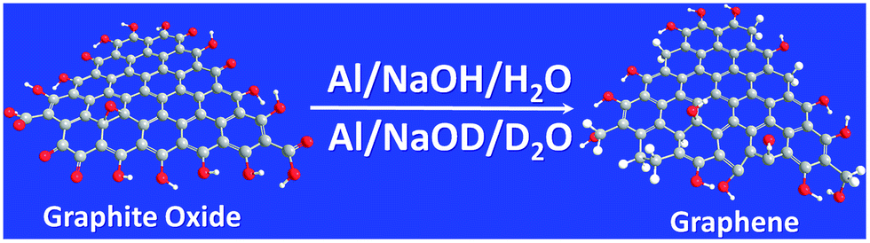

Scheme 1 Synthesis of hydrogenated graphene.

The morphology of reduced/hydrogenated graphene is shown in Fig. 1. The typical lamellar structure can be seen on all the samples. The slight differences in the structure and morphology resulted from differences in starting graphite oxide, for instance, for the graphene originating from HU-GO, more wrinkled samples are observed. SEM-EDS measurements were performed to obtain information about the elemental composition. In addition to carbon and oxygen, traces of aluminium and sodium were detected as well. These impurities originated from the synthesis procedure. The precise composition is summarized in Table 1.

Fig. 1 The surface morphology of graphene at various magnifications.

Table 1 Results of SEM-EDS in at.%

Sample	C	O	Na	Al
HO-OH	75.9	23.4	0.5	0.2
HO-OD	81.2	18.6	0.1	0.1
HU-OH	86.4	13.5	0.1	0.0
HU-OD	81.2	18.6	0.1	0.1

---

The composition and C/O ratio were measured using XPS. The survey spectra are shown in Fig. 2, which shows that both carbon (C 1s at ∼284.5 eV) and oxygen peaks (C 1s at ∼532 eV) are clearly visible. The XPS spectra of starting graphite oxide are shown in the ESI (Fig. SI1†). The obtained concentrations of carbon, oxygen and C/O ratios are summarized in Table 2. The C/O ratios in the range of 6–7 were observed for all the samples, except for the HU-OH sample with the ratio C/O = 3.8. Considering that the C/O ratio in the starting graphite oxide was 2.3 and 2.4 for HU-GO and HO-GO, respectively, all the resulting values are significantly higher compared to C/O ratios in the starting graphite oxide (∼2), indicating a successful reduction of graphite oxide. Except for carbon and oxygen, traces of sodium (up to 0.3 at.%) were also detected. The small peak at ∼370 eV can be attributed to the silver holder. Because no other elements were detected, we can conclude that no impurities are present in an amount sufficient to trap some significant amount of deuterium or hydrogen, (such as Al(OH)₃ or Al(OD)₃) and the deuterium detected in the reduced graphene thus originates dominantly from the C–D bonds.

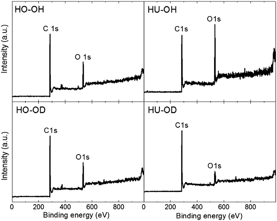Fig. 2 Survey spectra of hydrogenated graphene.

Table 2 The concentration of carbon and oxygen and C/O ratios obtained by XPS spectroscopy in atomic%

Sample	C [at.%]	O [at.%]	C/O
HO-OH	87.2	12.8	6.8
HO-OD	86.3	13.7	6.3
HU-OH	79.0	21.0	3.8
HU-OD	87.5	12.5	7.0

---

High resolution XPS was also used for further investigation of the chemical environment of the carbon and bonding characteristics of carbon atoms within graphene. The high resolution XPS spectra of C 1s peak are shown in Fig. 3. The deconvolution of C 1s peak was performed to estimate the concentration of various functional groups bonded to the carbon atoms. Energies of C=C bond at 284.4 eV, C–C and C–H at 285.4 eV, C–O at 286.3 eV, C=O at 288 eV, O–C=O at 289 eV and π–π* interactions at 290.5 eV were considered for the deconvolution. The results are summarized in Table 3 and can be compared with the results of C 1s peak deconvolution of the starting graphite oxide given in the ESI (Table SIA†).

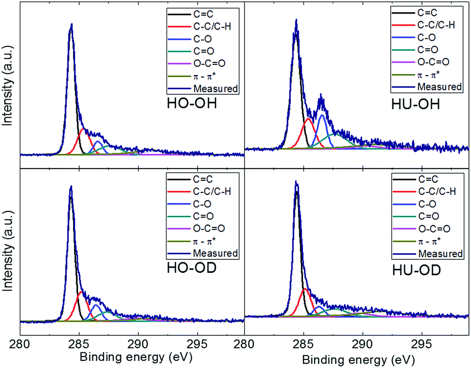Fig. 3 High resolution XPS spectra of the C 1s peak of hydrogenated graphene with fits of various carbon bonding states.

Table 3 The results of C 1s peak deconvolution with quantification of different carbon bonding states

Sample	C=C	C–O/C–H	C–O	C=O	O–C=O	π–π*
HO-OH	54.5	16.7	6.5	10.2	0.9	11.1
HO-OD	51.2	17.9	8.7	9.4	5.6	7.2
HU-OH	42.5	15.3	12.5	13.8	4.4	11.6
HU-OD	49.4	15.9	5.2	9.2	4.0	16.2

---

The elemental composition was investigated using elemental combustion analysis. The results in atomic percent are summarized in Table 4. A slightly lower concentration of hydrogen observed in deuterated samples is caused by the different molar mass of deuterium compared to hydrogen. The first indication of graphene hydrogenation originates from the H/O ratio. Because the H/O ratio corresponding to various oxygen functional groups is always less than or equal to unity (0.5 for carboxylic acids, 1 for hydroxyl groups and 0 for other oxygen functional groups such as epoxides and ketones), the value higher than 1 is a clear indication of C–H bond formation. For the rough estimation of minimum hydrogen concentration in the form of C–H group, we can use a simple subtraction of hydrogen and oxygen concentration. These results are also shown in Table 4. It should be noted that the composition of the starting graphite oxides was 46.65 at.% C, 22.08 at.% H and 31.27 at.% O for HO-GO and 43.39 at.% C, 24.61 at.% H and 32.00 at.% O for HU-GO.

Table 4 Composition in at.% of reduced/hydrogenated graphene obtained by elemental combustion analysis. Right column shows a minimal concentration of C–H bonds obtained from c_(C–H) = H − O

Sample	N	C	H	O	(C–H)
HO-OH	0.06	58.78	21.24	19.93	1.31
HO-OD	0.08	58.78	21.81	22.77	−0.96
HU-OH	0.19	54.92	22.31	22.58	−0.27
HU-OD	0.14	64.10	15.99	19.77	−3.78

---

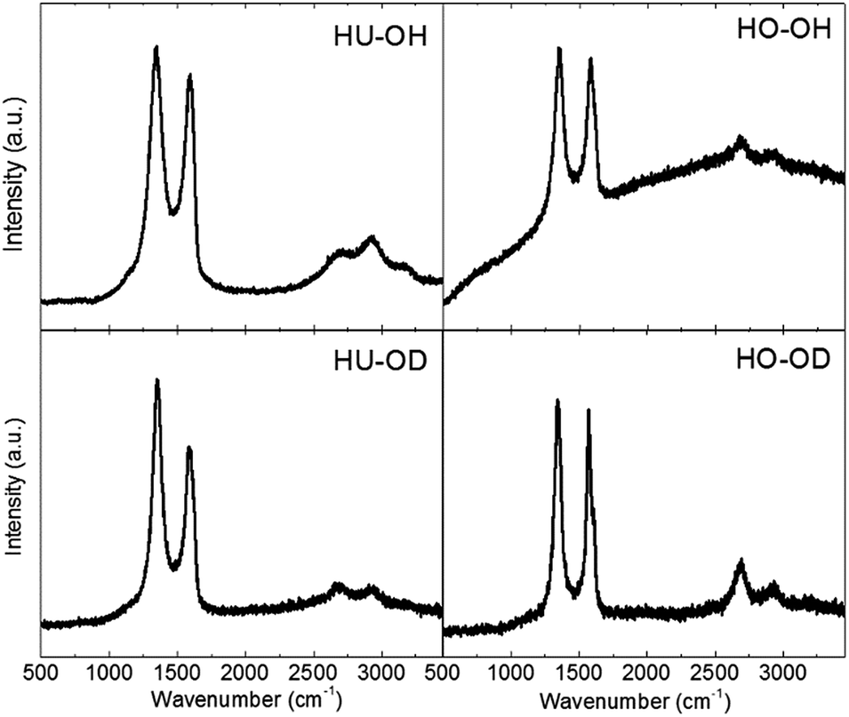
Another evidence for C–H bond formation can be obtained by FT-IR spectroscopy (Fig. 4). The C–H bands observed around 2920 and 2850 cm⁻¹ provide clear evidence of graphene hydrogenation. However, FT-IR spectra are significantly influenced by the high absorption of graphene, and only very weak intensities of bands are usually observed. In addition to this, we can see a broad vibration band for the hydroxyl functional group at 3400 cm⁻¹. This band, dominantly present in graphene, originates from the HO-GO precursor. A lower degree of reduction can be seen for the HU-OH sample, where an additional band corresponding to C=O functional groups can be seen at 1710 cm⁻¹. The vibration of the graphene skeleton originating from C=C bands is clearly visible at 1630 cm⁻¹. The broad vibration band at 1380 cm⁻¹ is related to the vibration of C–O bonds from remaining oxygen functional groups. For comparison, the FT-IR spectra of starting graphite oxides are shown in the ESI (Fig. SI2†).

Fig. 4 FT-IR spectra of reduced graphene.

Although all the above mentioned methods can give information about the presence of C–H, they cannot be used for exact quantitative determination of the hydrogen concentration in the form of C–H bond. To resolve this problem, we used a combination of ERDA and RBS (Fig. 5). The results of ERDA and RBS analysis of the starting graphite oxides are shown in the ESI (Fig. SI3†). Because ERDA is sensitive to light elements, it is very useful for the quantification of hydrogen and deuterium concentration. Moreover, RBS was used for the trace analysis of heavier elements.

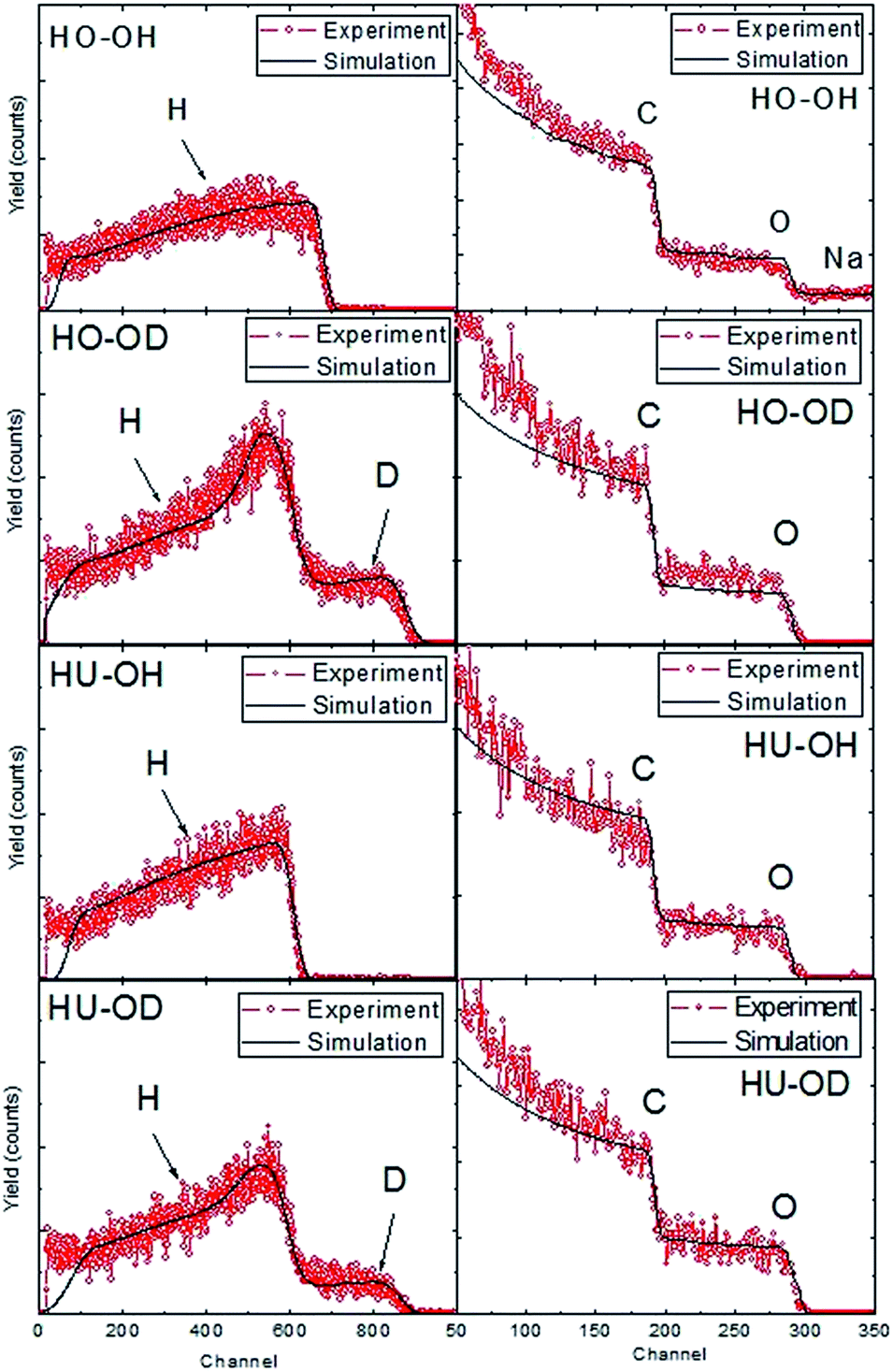Fig. 5 ERDA (left) and RBS (right) spectra of hydrogenated graphene.

The use of deuterated solvents and reactants led to the formation of deuterium labeled hydrogenated graphene. Subsequent treatment of such material with normal hydrogen led to deuterium exchange in all acidic groups such as hydroxyls or carboxylic groups. Only C–D bonds remained unchanged during this process and the exact determination of deuterium content yielded the extent of graphene hydrogenation/deuteration. The concentrations of hydrogen, deuterium, carbon and oxygen obtained by the combination of ERDA and RBS methods are summarized in Table 5. A higher degree of hydrogenation was observed for HO-OH and HO-OD samples. This is related to the different chemistry of HO-GO, where more reactive functional groups such as epoxides are present compared to HU-GO. These results are consistent with the data obtained by elemental combustion analysis showing a higher concentration of hydrogen in the form of C–H bond observed for the same samples.

Table 5 Concentrations of carbon, oxygen, hydrogen and deuterium measured by RBS (O and C) and ERDA (H and D) in at.%

Sample	C	O	H	D
HO-OH	73.4	18.1	6.5	0.0
HO-OD	71.3	12.6	9.3	6.8
HU-OH	73.2	12.9	13.9	0.0
HU-OD	72.3	14.9	9.5	3.3

---

The hydrogenated graphene was further investigated using Raman spectroscopy. Two main peaks located at 1560 and 1340 cm⁻¹ were found in the observed Raman spectra (Fig. 6). The peak located at 1560 cm⁻¹ (G-band) is associated with the sp² hybridized carbon atoms within hexagonal graphene framework. The peak at 1340 cm⁻¹ (D-band) is related to the carbon atoms with sp³ hybridization originating from the remaining oxygen functional groups and defects in the graphene layer. In addition, a weak peak observed around 2690 cm⁻¹ (2D-band) is associated with the number of layers. The intensities of D and G peaks are denoted as I_D and I_G, the ratio of their intensities corresponding to defects within the graphene structure. For the reduced/hydrogenated graphene, the following values were obtained: 1.28 for HU-OD, 1.10 for HU-OH, 1.03 for HO-OH and 1.04 for HO-OD. A higher degree of reduction and lower concentration of defects can be observed on samples prepared from HO-GO. This is in correlation with the composition of starting graphite oxide, where HU-GO contained a higher concentration of carboxylic acids and ketone functional groups. These functional groups were formed on the edges of graphene sheets and/or they were linked to defects within the graphene framework.

Fig. 6 Raman spectra of hydrogenated graphene.

In addition to chemical composition, the measurement of resistivity was performed. The resistivity of graphene samples is strongly correlated to the degree of reduction and concentration of the remaining functional groups. HO-OH and HO-OD exhibited resistivities of 1.42 × 10⁻² and 1.37 × 10⁻² Ω cm⁻¹, respectively, while for HU-OH and HU-OD, the respective values of 4.60 and 1.88 × 10⁻¹ Ω cm⁻¹, were attained. Samples with the highest degree of reduction revealed a lower specific resistivity. A significant difference was also found between the samples originated from various graphite oxides. Higher resistivity observed for samples synthesized from HU-GO was related to the higher concentration of defects, which was confirmed by Raman spectroscopy and by the higher concentration of oxygen functional groups.

To further investigate the remaining functional groups, the measurement of inherent electrochemistry in phosphate buffer was performed. Significant differences in the composition of the remaining oxygen functional groups between the hydrogenated graphenes were observed (Fig. 7). The electrochemical data show that there is a significant difference in the reduction efficiency between graphene oxides prepared by chlorate (HO) and permanganate (HU) methods in terms of residual electrochemically reducible groups (namely, epoxy, peroxy and aldehyde).²⁵ The reduction of HO-OH and HO-OD started at −0.67 and −0.57 V and reached the maximum at −1.28 and −1.51 V, respectively. In the case of HU-OH, the reduction started already at 0.13 V and culminated at −1.18 V. This result is in good agreement with other data obtained by XPS and FT-IR, where a relatively high concentration of remaining oxygen functional groups was observed in comparison with the other samples. The HU-OD sample exhibited a significantly higher degree of reduction. As a result, a weak reduction current was observed starting from −0.4 V, which was further increased at −1.16 V. However, no obvious reduction current maximum was observed for this sample.

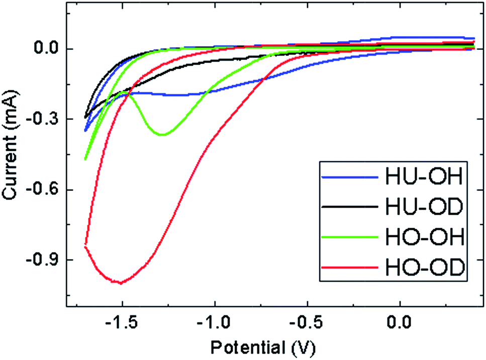Fig. 7 Inherent electrochemistry of hydrogenated graphene. (50 mM PBS, pH = 7.0, scan rate = 0.1 V s⁻¹).

Conclusions

The reduction with simultaneous hydrogenation of two different graphite oxides prepared by chlorate and permanganate routes was performed using aluminum powder in an alkaline environment. The hydrogenation of the reduced graphene was confirmed using FT-IR spectroscopy and elemental combustion analysis. Deuterium-labeled graphene was prepared using deuterium oxide and deuterated sodium hydroxide. Nuclear analytical methods, namely, RBS and ERDA, were used for the exact quantification of deuterium concentration within hydrogenated graphenes. Using a combination of these methods, we were able to measure the exact degree of hydrogenation. We showed that both graphene oxides prepared by permanganate and chlorate routes can be efficiently reduced and hydrogenated. Obtained results confirmed the successful synthesis of highly hydrogenated graphene, as well as the viability of deuterium-labeling technique as a highly efficient tool for the control of the hydrogenation of graphene at both laboratory and industrial scale.

Acknowledgements

The project was supported by Czech science foundation (Project no. 15-09001S) and by specific university research (MSMT no. 20/2015). RBS and ERDA analysis was realized at CANAM (Center of Accelerators and Nuclear Analytical Methods) LM 2011019. A.M. and R.M. were supported by the project P108/12/G108.

References

1. A. K. Geim and K. S. Novoselov, Nat. Mater., 2007, 6, 183–191.
2. R. R. Nair, W. Ren, R. Jalil, I. Riaz, V. G. Kravets, L. Britnell, P. Blake, F. Schedin, A. S. Mayorov, S. Yuan, M. I. Katsnelson, H.-M. Cheng, W. Strupinski, L. G. Bulusheva, A. V. Okotrub, I. V. Grigorieva, A. N. Grigorenko, K. S. Novoselov and A. K. Geim, Small, 2010, 6, 2877–2884.
3. O. Jankovský, P. Šimek, K. Klimová, D. Sedmidubský, S. Matějková, M. Pumera and Z. Sofer, Nanoscale, 2014, 6, 6065–6074.
4. O. Jankovský, P. Šimek, D. Sedmidubský, S. Matějková, Z. Janoušek, F. Šembera, M. Pumera and Z. Sofer, RSC Adv., 2014, 4, 1378–1387.
5. K.-J. Jeon, Z. Lee, E. Pollak, L. Moreschini, A. Bostwick, C.-M. Park, R. Mendelsberg, V. Radmilovic, R. Kostecki, T. J. Richardson and E. Rotenberg, ACS Nano, 2011, 5, 1042–1046.
6. M. Pumera and C. H. A. Wong, Chem. Soc. Rev., 2013, 42, 5987–5995.
7. J. O. Sofo, A. S. Chaudhari and G. D. Barber, Phys. Rev. B: Condens. Matter Mater. Phys., 2007, 75, 153401.
8. R. A. Schäfer, J. M. Englert, P. Wehrfritz, W. Bauer, F. Hauke, T. Seyller and A. Hirsch, Angew. Chem., Int. Ed., 2013, 52, 754–757.
9. A. Y. S. Eng, H. L. Poh, F. Šaněk, M. Maryško, S. Matějková, Z. Sofer and M. Pumera, ACS Nano, 2013, 7, 5930–5939.
10. Z. Yang, Y. Sun, L. B. Alemany, T. N. Narayanan and W. E. Billups, J. Am. Chem. Soc., 2012, 134, 18689–18694.
11. Z. Luo, T. Yu, K.-J. Kim, Z. Ni, Y. You, S. Lim, Z. Shen, S. Wang and J. Lin, ACS Nano, 2009, 3, 1781–1788.
12. H. L. Poh, F. Sanek, Z. Sofer and M. Pumera, Nanoscale, 2012, 4, 7006–7011.
13. Z.-J. Fan, W. Kai, J. Yan, T. Wei, L.-J. Zhi, J. Feng, Y.-M. Ren, L.-P. Song and F. Wei, ACS Nano, 2010, 5, 191–198.
14. X. Mei and J. Ouyang, Carbon, 2011, 49, 5389–5397.
15. Z. Sofer, O. Jankovský, P. Šimek, L. Soferová, D. Sedmidubský and M. Pumera, Nanoscale, 2014, 6, 2153–2160.
16. Z. Fan, K. Wang, T. Wei, J. Yan, L. Song and B. Shao, Carbon, 2010, 48, 1686–1689.
17. O. Jankovský, P. Šimek, D. Sedmidubský, Š. Huber, M. Pumera and Z. Sofer, RSC Adv., 2014, 4, 7418–7424.
18. U. Hofmann and A. Frenzel, Kolloid-Z., 1934, 68, 149–151.
19. W. Hummers and R. Offeman, J. Am. Chem. Soc., 1958, 80, 1339.
20. C. H. A. Wong, O. Jankovský, Z. Sofer and M. Pumera, Carbon, 2014, 77, 508–517.
21. J. Saarilahti and E. Rauhala, Nucl. Instrum. Methods Phys. Res., Sect. B, 1992, 64, 734.
22. M. Mayer, SIMNRA version 6.06, Max-Planck-Institut fur Plasmaphysik, Garching, Germany, 2011, available at: http://home.rzg.mpg.de/%7Emam/Download.html.
23. IBANDL, http://www-nds.iaea.org/ibandl/.
24. L. J. van der Pauw, Philips Tech. Rev., 1958, 20, 220–224.
25. E. L. K. Chng and M. Pumera, Chem.–Asian J., 2011, 6, 2899–2901.

---

Footnote

† Electronic supplementary information (ESI) available. See DOI: 10.1039/c4ra16794e

---