Estimation of the uncertainty of the measurement results of some trace levels elements in document paper samples using ICP-MS

Abstract

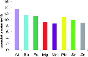
The measurement uncertainty characterizes the dispersion of the quantity values being attributed to the measurand and there are different approaches for uncertainty estimation. This study illustrates the application of the GUM (bottom-up) approach to estimate the measurement results uncertainty for the quantitative determination of Al, Ba, Fe, Mg, Mn, Pb, Sr and Zn from document paper samples using ICP-MS. The measurement uncertainty estimation was done based on identifying, quantifying and combining all the associated sources of uncertainty separately. Certain typical steps were followed: specifying the measurand; identifying the major sources of uncertainty; quantifying the uncertainty components; combining the significant uncertainty components; determining the extended combined standard uncertainty; reviewing the estimates and reporting the measurement uncertainty. For the eight mentioned trace elements the combined standard uncertainties and the expanded uncertainties were determined. The relative measurement uncertainty values lay between 7.7% and 13.6%. In all the five paper samples for each of the eight elements homogenous uncertainty values were obtained. In order to emphasize the uncertainty sources contributions, the percent contribution of the uncertainty components to the combined relative standard uncertainty were graphically represented for the elements determined by ICP-MS in paper samples. The previously validated method proved to be suitable for the intended purpose and when the uncertainty of the measurement results is estimated, it becomes a significant tool for characterizing the elemental composition of the document paper samples. Moreover, the applied approach for the uncertainty estimation enables improving the data quality and decision making.

---

1 Introduction

For most products, processes and services the quality represents the main decision factor of the user's choice. The quality leads to competitiveness and improves the economy. Analytical chemistry has always been used to assess the quality of the products manufactured in various industries (chemical, pharmaceutical, food, metallurgical, etc.). Before reporting the results, an analytical chemist has to evaluate their reliability.¹

The result of a chemical measurement can be altogether interpreted only when this is accompanied by its established measurement uncertainty. The uncertainty is necessary to decide whether the measurement result is fitted for the intended purpose and to prove that is consistent with other similar results.

The errors that affect all the measurements are not fully corrected for, so the results differ from the true value of the measurand. Many sources of the measurements errors can be identified and the errors can be quantified and corrected (using the calibration certificates). Nevertheless, are seldom available the time and resources to entirely determine the errors and apply the corrections.

The measurement uncertainty is a quantitative measure of a measurement result quality that allows the comparison with other results, references, standards, etc. The measurement uncertainty is “a non-negative parameter associated with the result of a measurement that characterizes the dispersion of the quantity values that could reasonably be attributed to the measurand”.² The parameter may be a standard deviation or half-width of an interval with a stated level of confidence. The uncertainty denotes the level of confidence that the value lies within the interval, when it is estimated and reported in a stated manner.

The error is a single value and represents the difference between the result and the “true” value of the measurand. The error cannot be exactly determined because the “true” value is not really known, but only the “most probable value”.

The uncertainty is reported as an interval and in certain conditions it can be applied to all further measurements. The measurement result cannot be corrected using the uncertainty, but using the error value a correction of the result can be done. After correcting any known errors, there are some that still remain unknown. These represent sources of uncertainty.

On the other hand, the uncertainty is a quantification of the doubt about the result, but increases the confidence in the validity of that result.

Wernimont³ published in the mid 80's one of the first approaches to uncertainty estimation in analytical chemistry, using the precision estimates from inter-laboratory studies for uncertainty estimation.

Currently, the most important general approaches for estimating the measurement uncertainty are: (1) bottom-up approach (GUM); (2) top-down approach based on interlaboratory data; (3) top-down approach based on in house validation data.

Bottom-up or error-budget or error propagation approach was proposed in the guide to the expression of uncertainty in measurement (GUM).⁴ Here the uncertainty of the measurement result is obtained by combining the contributions of all the uncertainty sources. GUM was adopted for analytical chemistry by EURACHEM.⁵ The measurement uncertainty estimation in quantitative chemical analysis was applied in various studies^6–20 and it can be considered as common practice. It is also a requisite for the implementation of ISO/IEC International Standard 17025 (ref. 21) in laboratories. Because it is not easy at all to combine all sources of uncertainty, analytical chemists hesitate to adopt this approach.

The Analytical Methods Committee (AMC) of the Royal Society of Chemistry introduced the top-down approach based on an inter-laboratory study²² and the Nordic Committee for Food Analysis (NKML) an approach based on intra-laboratory data.²³ It must be mentioned that most of the data for the top-down approach are usable from the method validation.

The paragraph from ISO 17025 (ref. 21) that says “reasonable estimation shall be based on knowledge of the performance of the method and on the measurement scope and shall make use of, for example, previous experience and validation data” explicitly refers²⁴ to GUM⁴ and ISO 5725-2.²⁵ In the second edition of the EURACHEM guide²⁶ is also suggested to use the validation data in the uncertainty estimation. This is stated as well in an IUPAC project²⁷ that mentions that the data from robustness tests can help to the uncertainty estimation.

Over time it was emphasized that the information obtained from fulfilling the quality control and from validation studies should be supported by the estimation of measurement uncertainty.^4,28 Information regarding the performance parameters of the analytical method and the sources of uncertainty (identified and separately quantified) are combined and underlies the uncertainty estimation approach that has been applied in several studies.^29–32

The robustness data were used to complete the precision and trueness data in a bottom-up approach for the uncertainty estimation by Barwick and Ellison,¹⁰ including more sources of uncertainty.

While for the primary analytical chemical methods (titrimetry and isotope dilution mass spectrometry) bottom-up approach has been demonstrated,²⁴ for the more complicated ones, it is more difficult to combine all the relevant uncertainty sources.

The uncertainty of a certain measurement result can be really estimated only when are known all the uncertainties arising from the measurement procedure³³ and all the uncertainties associated with the references (standards) that the analytical results are made traceable to.³⁴

Currently, there are various approaches for the overall measurement uncertainty estimation, reviewed by different authors:^24,35,36 bottom-up, error-budget, error-propagation or component-by-component approach;^5,37 top-down approach;²² validation-based approach;^5,10 fitness for purpose approach;³⁸ robustness-based;^24,32 accuracy profile approach;^39,40 differential approach.⁴¹

In the traditional approach, namely bottom-up approach, the overall uncertainty is obtained by identifying, quantifying and combining all individual contributions to uncertainty. Initially developed for physical measurements this approach was adopted by EURACHEM for the chemical measurements.⁵ Because it is complex, this approach necessitates significant effort, is expensive and time consuming.

The fitness-for-purpose approach is simpler and uses a single parameter (the fitness function) with a form of an algebraic expression u = f(c) that represents the correlation between the measurement uncertainty and the concentration of the analyte. In this case, the estimation of the measurement uncertainty is based on the method performance characteristics (repeatability and reproducibility precision, and bias).⁴² This approach can be considered a simplification of the step-by-step approach, as described by EURACHEM.²⁶

Measurement uncertainty can be estimated using the data obtained during the method validation (includes method-performance studies):^22,38,43 data from in-house and collaborative validation studies, proficiency-testing schemes or quality assurance data. Quality control measures and validation studies are very useful for estimating measurement uncertainty^22,44 and there were already mentioned three approaches that are based on validation data.

The top-down approach²² considers a laboratory as part of a population of groups and the systematic errors within that laboratory become random errors. Therefore, the estimated uncertainty is the reproducibility uncertainty. This approach was applied and reported in different papers.^45–47 The validation based approach and robustness based approach use various method-performance parameters. In the former inter- or intra-laboratory validation studies (precision, trueness, robustness) are used. The latter is based on intra-laboratory simulations of inter-laboratory studies. All three validation-based approaches for measurement uncertainty estimation represent a validation widening.

Applying the differential approach can be developed detailed models of the performance of complex measurements, allowing the assessment of the individual precision components of the various analytical steps.⁴¹

In the present study measurement uncertainty is estimated using the GUM bottom-up approach. The analytical method was developed and validated for simultaneous determination of 8 elements (Al, Ba, Fe, Mg, Mn, Pb, Sr, Zn) from document paper using inductively coupled plasma-mass spectrometry (ICP-MS).^48,49

2 Experimental

Materials

For washing the glassware and for the preparation of all the solutions ultra-pure de-ionized water from a Milli-Q analytical reagent grade water purification system (Millipore, USA) was used. All the reagents and solvents were of analytical grade: nitric acid (Merck, suprapur), hydrogen peroxide (BDH Prolabo, 30%).

To prepare the instrument for the analysis a multi-element solution is used (PerkinElmer Co., Beaconsfield, Bucks, UK, plasma degrees, which contains Be, Co, In, Ge, Tl and U, 10 μg L⁻¹ for each element), prepared in 2% w/w HNO₃.

The calibration standard solutions and internal standard solutions were prepared using a certified reference material (ICP Multi Element Standard Solution, XXI Certi Pur Lot No HC 001232, Merck, 25 elements of 10 mg L⁻¹ each). Using this stock solution the calibration standard solutions were prepared in 2% w/w HNO₃ (in 25 mL volumetric flask), their concentrations lying between 5 and 100 μg L⁻¹.

The paper samples for the analysis were office document paper: white, A4 (210/297 mm), 80 g m⁻² printer/copy paper labeled acid- and chlorine-free. Five different brands of paper were used: 1 – STORAENSO, multilaser; 2 – XEROX, business; 3 – UNI COPY, laser copier; 4 – NAVIGATOR, universal; 5 – SKY COPY, paper.

Apparatus

All the measurements were performed using NexION 300 ICPMS (Perkin Elmer Co., Beaconsfield, Bucks, UK) with S10 auto sampler. The spectral data were processed with the ChromeraR (Perkin Elmer Co., Beaconsfield, Bucks, UK). For the digestion of the samples a microwave digestion unit (MW 3000 PerkinElmer) was used.

Brief description of ICP-MS

The emergence, development and use of the plasma torch as an excitation and ionization source in spectrometry produced an impressive development in the field of analytical elemental analysis. Nowadays, ICP-AES and ICP-MS are essential analytical techniques for chemists that use them in various areas.^50–53

A useful analytical technique requires simple spectra, appropriate spectral resolution and low detection limits. That is the reason for which a mass spectrometer was used as a detector and high pressure plasma as an ion source. Initially, a direct current plasma at atmospheric pressure was used, the obtained temperature (4000 K) producing an ionization yield of more than 50% for most elements.^54,55 Various studies of atmospheric pressure chemical flames were made.^56,57 Further, when pneumatic and ultrasonic nebulizers were used,⁵⁷ two shortcomings appeared: the presence of the severe matrix interferences due to the low temperature (3000 K) of the sample in the direct current plasma; the lack of the effective ionization of the elements with an ionization potential higher than 8–9 eV. In the case of the inductively coupled plasma these two disadvantages are really diminished, the temperature being of 7000 K or even higher. ICP was introduced as an ion source for mass spectrometry by Fassel and Houk in the USA and Gray and Date in the UK.^58,59 Another ion source for mass spectrometry was the microwave induced plasma, used by Douglas and French.⁶⁰

As a consequence of using mass spectrometry detection the operating conditions for this type of detector must be known. The processing of ions from inductively coupled plasma and the ion beam transportation in a mass spectrometer means the conversion of the conditions from the atmospheric pressure and the high temperature of the ICP ion source to the vacuum conditions and room temperature, required in mass spectrometry, preferably without changing the sample composition.

The interface between the ICP and the mass spectrometer is the key part of an ICP-MS instrument and it is crucial for its analytical performance. The ICP-MS appeared when the continuous extraction of the ions from the plasma volume was possible without any influence from the boundary layers. It was necessary a deep insight in terms of analytical performance of the modern ICP-MS instruments and of induced interference.

Nowadays, ICP-MS is widely used in the ultra-trace analysis of different samples. ICP-MS instruments prove detection limits at ng L⁻¹ level for many elements. The linear dynamic range of 4 to 5 orders of magnitude and the ability to do multi-element analysis are also excellent analytical features for ICP-MS.

The direct determination of major constituents by ICP-MS is often difficult because the analytes with concentrations above 1 mg L⁻¹ cause the detector saturation. Thus, when it is required to determine both major and trace elements, the major constituents must be separately determined by ICP-AES (directly) or by ICP-MS after sample solution dilution and then the trace elements are determined by ICP-MS. Such separate measurements are time consuming. In addition, the separate determination of major and trace elements presents difficulties when the analysis is done with limited sample amounts. As a factor that restricts the upper limit of the ICP-MS determinations is the conventional detector saturation (secondary electrons multiplier, which operates in ion counting mode), some commercial ICP-MS instruments have a less sensitive detector in order to extend the dynamic range towards higher concentrations.

Taking into consideration the operating system of the mass spectrometer, it is necessary plenty of time to change the sensitivity of the detector and the operating conditions. Therefore, the determination of analytes with high, respectively low concentrations in a single measurement is not possible in an alternative method.

Almost the same inductively coupled plasma or argon torch is used as ions source in ICP-MS and as radiation source in ICP-AES. Thus, the construction of a combined system (ICP-MS with ICP-AES) with a single plasma torch enables the fast, simultaneous multi-element determination over a wide range of concentrations (ng L⁻¹ to mg L⁻¹). Using such a system leads to reduced consumption of argon, the gas used for measurements in ICP-MS and ICP-AES.

From the point of view of applied analysis, ICP-MS is inclined towards isobaric and polyatomic interferences, as well as to the matrix effect, while ICP-AES often presents some spectral interference. Therefore, both in ICP-MS and ICP-AES such interference leads to analytical results submitted to errors, irrespective of the different causes of the interference from a technique to another. A combined system (ICP-MS and ICP-AES) is useful for the comparison of the analytical data obtained by two independent methods for analytes with μg L⁻¹ concentrations.

The ICP-MS method for which the estimation of the uncertainty of the measurement results is described in this paper was developed for multi-element analysis for quantitative determination of eight chemical elements (Al, Ba, Fe, Mg, Mn, Pb, Sr, Zn) in documents paper samples. This method is suitable for comparing document sheets, being fast, accurate and precise, allowing the analysis of trace elements at low levels of concentration (ng L⁻¹).

Measurement uncertainty estimation for trace levels elements in paper by ICP-MS using GUM approach

Over time, in the exact sciences and metrology appeared questions about the measurement results accuracy. The answers were related to the systematic and random measurement errors and can be argued due to the lack of modern data processing technology. The continuous development of these methods leads to a new point of view. In the first approach the random and systematic measurements errors were related to the “true value” of a quantity, which not only that is not really known, but finding it represents the goal of any measurement. Precisely because of reporting the errors to the “true value”, this must be known before the measurement.⁶¹

The concept of “measurement uncertainty” was first introduced by the physicists and later was adopted by the chemists. By publication of the “Guide to the expression of uncertainty in measurement – GUM”⁴ by ISO in collaboration with BIPM, IEC, IPCC, IUPAC, IUPAP and OIML the general rules for estimating the measurement uncertainty were established.

The first edition of the EURACHEM Guide “Quantifying uncertainty in analytical measurement – QUAM”⁵ published in 1995 shows how ISO GUM concepts can be applied in the chemical measurements.

GUM approach⁴ for uncertainty estimation, also known as “bottom-up”, “error-budget”, “error propagation” or “component by component”^4,5,33,46 refers to the identification, estimation, quantification and combination of all the measurement uncertainty sources.

A quantity X can be represented by a probability distribution, as was proved by Weise and Wöger⁶² using the theory of probabilities and statistics.

The best estimate derived from the distribution is the expectation of the distribution and the measurement uncertainty is its standard deviation:

x = E[X] (1)

This uncertainty is standard measurement uncertainty not only because it represents the standard deviation of the distribution, but also because expresses the mean width of the distribution.

The current estimation of the uncertainty in the GUM approach (the classical one) is based on a model equation that provides a unique relationship in most cases between the measurand Y and N input quantities X₁, X₂, …, X_N, expressed as:^4,5

Y = f(X₁, X₂, …, X_N) (3)

The expectation values of the distributions are:

x₁ = E[X₁], x₂ = E[X₂], …, x_N = E[X_N] (4)

Evaluating these best estimates and using the evaluation model, the value of the result quantity is determined:

y = f(x₁, x₂, …, x_N) (5)

First, the standard measurement uncertainties of the input values are calculated based on the variances of the distributions. After that, the standard measurement uncertainty of the result is obtained using the uncertainty contributions and the correlation coefficients. Finally, the combined standard measurement uncertainty of the result u_c(y) is calculated as:

where u²(x₁), u²(x₂), …, u²(x_N) are the uncertainty contributions and are the sensitivity coefficients.

The values and the standard measurement uncertainties for the input quantities are determined using two types of evaluation methods: A type method and B type method.

In the A type evaluation method to obtain the standard measurement uncertainty statistical procedures are used. That is when various values are obtained for different measurements under the same conditions.

The B type method is based on the procedures of the theory of probability and is done when: data from previous measurement are available; sufficient information is known about the measuring instruments or materials; specifications of the manufacturer and different certificates are available.

3 Results and discussions

In the present study, the measurement uncertainty of the measurement results for determination of trace elements from document paper using inductively coupled plasma-mass spectrometry (ICP-MS) was estimated using GUM⁴ and EURACHEM⁵ “bottom-up” classical approach.

In order to obtain an estimate of the output quantity and of the corresponding standard uncertainty using the values of the input quantities and theirs standard uncertainties, the contributions of all the significant uncertainty sources were taken into consideration. As was already mentioned above, both type A and type B evaluation methods are applied and in the end the standard uncertainty and the expanded uncertainty of the result are presented. The approach that models the measuring process is helpful for the uncertainty estimation and it is used in various situations in real practice.²⁰

Accomplishing the estimation of the measurement uncertainty using the “bottom-up” approach requires a significant effort, so a balance must be created between the time and money spent on the one hand and the “gains” obtained on the other hand.¹⁰ When validation data are available for a certain method, the uncertainty estimation can be easier done so the requirements from the ISO/IEC 17025 standard²¹ are fulfilled.

To obtain the measurement uncertainty the next steps are recommended to be followed:^18,63 (1) specifying the measurand; (2) identifying the major sources of uncertainty; (3) quantifying the uncertainty components; (4) combining the significant uncertainty components; (5) expansion of the combined standard uncertainty; (6) reviewing the estimates and reporting the measurement uncertainty.

In the first step a clear statement of what should be measured it is necessary to be written. The analysis method was developed and characterized previously, so the measurand specification is done best by a description of the different steps of the analytical method and by establishing the measurand defining equation. GUM states that the measurand cannot be specified through a value, but only by a quantity description, so for the complete description of the measurand it is required a large amount of information.

In the present study the measurand is the mass fraction for each of the eight elements (Al, Ba, Fe, Mg, Mn, Pb, Sr, Zn) estimated in document paper samples using ICP-MS, following the procedure presented in Fig. 1.

Fig. 1 Flow diagram for the analysis of trace elements in paper samples by ICP-MS.

A flow diagram is easily done when a standard operating procedure is available. The latter one helps to the better understanding of the analytical test procedure. Such a flow diagram is not compulsory, but is very useful irrespective of the uncertainty estimation approach, but especially when using “bottom-up” approach. Fig. 1 shows a flow diagram of the procedure for the analysis of trace elements in paper samples by ICP-MS.

The equation used to obtain the measurand is:

where w is the measurand, namely the mass fraction of an element in the sample (μg g⁻¹), γ₀ is the mass concentration of an element in the digested sample (μg L⁻¹), V_s is the digested sample volume, m is the digested sample mass, f_D is a dilution factor.

All the parameters that influence the measurements results (the second step) are very well highlighted when are depicted on a cause-effect diagram (Ishikawa diagram or fishbone diagram) (Fig. 2).

Fig. 2 General Ishikawa diagram presenting the uncertainty sources of the measurement uncertainty.

Not all the uncertainty sources can be identified. There are taken into consideration only those with significant contributions to the final uncertainty, such as: recovery, calibration, standard solutions preparation, purity, mass sample, etc. The detailed equation of the measurand is the starting point of the Ishikawa diagram and these two must be always compared (each factor of the equation should appear on the diagram).

In the third step, namely the quantification of the uncertainty sources, the uncertainty components magnitude is estimated. Often is possible to be estimated only one contribution to the uncertainty, associated with a certain number of sources.

It must be mentioned that the standard uncertainties u(x) can be standard deviations. These are obtained by repeated measurements, are representative for the normally distributed data and they show the data spreading:

Standard deviation of the mean can also be calculated:

and can be used only if it is applied to a well-defined and finished process.

In certain conditions the standard uncertainty is not determined as standard deviation by repeated measurements, but by other type of distribution. The most commonly distributions used by QUAM⁵ are the rectangular and triangular ones, both of them having defined limits.

The rectangular distribution is used where the probability of obtaining any value between two limits is equal to the probability of obtaining any other value or, in another words, there is an equal probability of a measurement occurring within the bound limits. This kind of distribution is associated with manufacturer specifications. The GUM recommends using the rectangular distribution when the frequency distribution is not known.

The triangular distribution is used where there is a tendency for the values to be near the center of the distribution and not at the extremes. This type of distribution applies for the volume of a measuring flask. If the given volume of a flask is (250 ± 0.1) mL, then the standard uncertainty is .

To obtain the combined standard uncertainty of the measurand u_c(M) some calculation rules are followed.¹⁸ For the measurand M the equation is established, then u_c(M) is calculated as:

where u(x_i) are the standard uncertainties of the individual uncertainty sources. eqn (10) is only applicable to independent components. In many cases this equation becomes simpler, for example when the equation for the measurand is M = (a × b)/(c × d). Then eqn (10) becomes:oru_c(M)/M represents the relative uncertainty (dimensionless) and u_c(M) is the absolute uncertainty (with the same unit as M).

These calculations usually apply to the bottom-up approach and they are thorough. An alternative method for u_c(M) determination is the Monte Carlo simulation method.⁶⁴ This methodology involves the propagation of the uncertainty input sources distributions (and not the propagation of the uncertainties) by using the model to provide the distribution of the output. It is an experimental probabilistic method that requires the availability of computers with a certain configuration and its application to uncertainty estimation can provide a realistic approach. Monte Carlo simulations have the advantage that there are obtained results for a wider range of models. Although it can address higher complexity measurement equations, the practical use of this method is still relatively restricted.

Returning to the main uncertainty sources, the volumetric operations are going to be taking first into consideration. The uncertainty sources for the uncertainty of the volume of a pipette, burette or a volumetric flask are: calibration, repeatability and temperature.

Calibration

In the case of the calibration uncertainty for a pipette, burette or a volumetric flask a triangular distribution is applied and is provided by the manufacturer. For example, for a 2 mL pipette the manufacturer provides the information (2 ± 0.01) mL (at 20 °C). Standard uncertainty will be:

Repeatability

The repeatability presents a normal distribution and the standard deviation can be calculated after fulfilling the required experiments. For the 2 mL pipette the repeatability uncertainty is:

u(V_rep) = s_rep = 0.0023 mL (13)

Temperature

As already mentioned above, the temperature influence presents a rectangular distribution. According to the manufacturer, the 2 mL pipette was calibrated at 20 °C and the laboratory temperature varies with ±4 °C. The standard uncertainty is calculated as:where γ is the coefficient of the volume expansion of the liquid.

The relative standard uncertainty for the 2 mL pipette is:

Similarly, the volume standard and relative uncertainties were calculated for all the used pipettes, burettes and volumetric flasks. The relative combined standard uncertainty for the volume with the dilution D was calculated:

All the obtained results are presented in Table 1.

Table 1 The volume uncertainty

Item	The volume (mL)	Calibration uncertainty	Repeatability uncertainty urep(V) = srep	Temperature uncertainty	The standard uncertainty	The relative standard uncertainty	The relative combined standard uncertainty
Pipette	1	0.0029	0.0015	0.0005	0.0033	0.0033	0.0059
Pipette	2	0.0041	0.0023	0.0010	0.0048	0.0024
Pipette	5	0.0123	0.0049	0.0024	0.0134	0.0027
Pipette	10	0.0204	0.0068	0.0049	0.0221	0.0022
Volumetric flask	25	0.0245	0.0065	0.0121	0.0281	0.0011
Volumetric flask	50	0.0327	0.0085	0.0243	0.0416	0.0008
Volumetric flask	100	0.0408	0.0200	0.0485	0.0665	0.0007
Volumetric flask	500	0.1021	0.0683	0.2425	0.2718	0.0005
Volumetric flask	1000	0.1633	0.0888	0.4850	0.5194	0.0005
Burette	10	0.0123	0.0065	0.0049	0.0147	0.0015
Burette	25	0.0184	0.0132	0.0121	0.0257	0.0010

---

Weighing

For the mass determinations the uncertainty sources are: the repeatability, the non-linearity of the response curve, the sensitivity, the temperature coefficient.⁶⁵ Although there are some complex correlations, the weighing uncertainty is usually rather small.

For the weighing of a sample (with mass m) the following uncertainty sources were taken into consideration: the repeatability; the balance drift from the calibration certificate; the temperature coefficient.

The equation used for the weighing uncertainty calculation is:

where: m is the value of the weighed sample (m = 5 g and s = 0.0817 mg for 10 repeated weighings); u_m,rep is the uncertainty due to the repeatability (it is taken into consideration twice because of the tare weigh and represents the standard deviation); u_m,cal is the calibration uncertainty (rectangular distribution); u_m,temp is the uncertainty due to the temperature variations (rectangular distribution), calculated as:where: K is a constant from the balance certificate (1.5 × 10⁻⁴/°C) and ΔT represents the temperature variation between the calibration and the weighing (±4 °C).

Therefore, the weighing uncertainty is:

The relative standard weighing uncertainty will be:

The purity of the standards and the reference materials must be considered irrespective of the uncertainty estimation approach that it is used. The obtained results will depend on the purity degree of the reference.

In the certificate of the reference material are always found some kind of information: the degree of purity, a specification about the analyte content or the uncertainty of the certified value as a confidence interval. In the present paper was applied the latter case: (9.9 ± 0.5) mg L⁻¹. So the standard uncertainty used in the calculation was obtained using the following equation:

where: u(P) is the purity uncertainty.

The relationship between the purity P and the relative standard uncertainty is given by:

From this equation P was determined as 0.94665.

The relative standard uncertainty for the purity of each analyte (Al, Ba, Fe, Mg, Mn, Pb, Sn, Zn) from the ICP Multi Element Standard CertiPur Solution is:

u(P)/P = 0.0308 (23)

The uncertainty of the calibration function can be determined using different approaches and equations as long as the variations of the signals are much higher than those of the concentrations. Some of those equations are presented in QUAM.⁵

The calibration step influences the combined uncertainty of the sample result. Calibration standard uncertainty should be included in the uncertainty budget.

In the calibration step there are four uncertainty sources that can influence the standard uncertainty of a single measurement:^66,67 repeatability of reading the signal value for standard solutions and for the sample; uncertainty due to the determination of the reference value for the standard solutions; the effect of the standard solutions preparation, the approximations made using a regression curve.

The sample signal is fitted to the calibration function obtained using the calibration standards, mostly based on the least square linear regression, which assumes: the validity of the linear model; that the response is a random variable with constant variance; that the analyte concentrations in standard solutions are known with a negligible magnitude of the associated uncertainty. The equation for the linear model is:

y = a + bx + ε (24)

where: a is the intercept, b is the slope and ε is a normally distributed random variable.

Calculating the regression parameters, the regression curve uncertainty can be estimated. Standard uncertainty due to the uncertainty of calibration and linear regression method u(c_cal) is determined as:

where: s_xy is the residual standard deviation, b is the slope of the calibration curve, p is the number of measurements for a certain sample, n is the total number of standard solutions in the calibration curve, c_sample is the mean of all the concentrations of a standard solution for which the measurements were made, c̄ is the mean concentration of all the standard solutions and .

The calibration relative standard uncertainty values for the eight elements (Al, Ba, Fe, Mg, Mn, Pb, Sr, Zn) determined by ICP-MS are presented in Tables 2–6.

Table 2 The combined standard uncertainties u_c(w) and the expanded uncertainties U for the eight elements (Al, Ba, Fe, Mg, Mn, Pb, Sr, Zn) determined by ICP-MS in paper 1 sample^a

Element	Uncertainty
								uc(w) (μg g^−1)	U/w (%)	w ± U (μg g^−1)
a m – weighing, D – volume, P – purity, R – recovery, r – repeatability, ccal – calibration, w – measurand.
Al	0.0003	0.0059	0.0308	0.0040	0.0405	0.0445	0.0680	12.57	13.6	185 ± 25.14
Ba	0.0003	0.0059	0.0308	0.0038	0.0405	0.0251	0.0572	0.57	11.4	10 ± 1.14
Fe	0.0003	0.0059	0.0308	0.0084	0.0434	0.0109	0.0553	6.94	11.1	125.6 ± 13.88
Mg	0.0003	0.0059	0.0308	0.0048	0.0213	0.0247	0.0455	24.26	9.1	533 ± 48.51
Mn	0.0003	0.0059	0.0308	0.0017	0.0284	0.0097	0.0434	0.18	8.7	4.26 ± 0.37
Pb	0.0003	0.0059	0.0308	0.0017	0.0436	0.0077	0.0543	0.01	10.9	0.24 ± 0.03
Sr	0.0003	0.0059	0.0308	0.0068	0.0365	0.0091	0.0494	1.26	9.9	25.4 ± 2.51
Zn	0.0003	0.0059	0.0308	0.0014	0.0281	0.0150	0.0447	0.04	8.9	0.92 ± 0.08

---

Table 3 The combined standard uncertainties u_c(w) and the expanded uncertainties U for the eight elements (Al, Ba, Fe, Mg, Mn, Pb, Sr, Zn) determined by ICP-MS in paper 2 sample^a

Element	Uncertainty
								uc(w) (μg g^−1)	U/w (%)	w ± U (μg g^−1)
a m – weighing, D – volume, P – purity, R – recovery, r – repeatability, ccal – calibration, w – measurand.
Al	0.0003	0.0059	0.0308	0.0028	0.0382	0.0445	0.0666	14.22	13.3	213.6 ± 28.43
Ba	0.0003	0.0059	0.0308	0.0013	0.0331	0.0251	0.0520	0.34	10.4	6.46 ± 0.67
Fe	0.0003	0.0059	0.0308	0.0098	0.0271	0.0109	0.0439	9.90	8.8	225.4 ± 19.81
Mg	0.0003	0.0059	0.0308	0.0091	0.0165	0.0247	0.0441	31.42	8.8	711.8 ± 62.84
Mn	0.0003	0.0059	0.0308	0.0024	0.0294	0.0097	0.0441	0.26	8.8	5.86 ± 0.52
Pb	0.0003	0.0059	0.0308	0.0002	0.0374	0.0077	0.0494	0.05	9.9	0.98 ± 0.10
Sr	0.0003	0.0059	0.0308	0.0057	0.0384	0.0091	0.0507	1.96	10.1	38.64 ± 3.92
Zn	0.0003	0.0059	0.0308	0.0003	0.0433	0.0150	0.0555	0.32	11.1	5.82 ± 0.65

---

Table 4 The combined standard uncertainties u_c(w) and the expanded uncertainties U for the eight elements (Al, Ba, Fe, Mg, Mn, Pb, Sr, Zn) determined by ICP-MS in paper 3 sample^a

Element	Uncertainty
								uc(w) (μg g^−1)	U/w (%)	w ± U (μg g^−1)
a m – weighing, D – volume, P – purity, R – recovery, r – repeatability, ccal – calibration, w – measurand.
Al	0.0003	0.0059	0.0308	0.0046	0.0264	0.0445	0.0607	13.82	12.1	227.8 ± 27.65
Ba	0.0003	0.0059	0.0308	0.0021	0.0393	0.0251	0.0562	0.10	11.2	1.8 ± 0.20
Fe	0.0003	0.0059	0.0308	0.0038	0.0258	0.0109	0.0422	4.79	8.4	113.6 ± 9.58
Mg	0.0003	0.0059	0.0308	0.0100	0.0097	0.0247	0.0423	43.05	8.5	1018 ± 86.10
Mn	0.0003	0.0059	0.0308	0.0022	0.0371	0.0097	0.0496	0.33	9.9	6.74 ± 0.67
Pb	0.0003	0.0059	0.0308	0.0020	0.0415	0.0077	0.0527	0.04	10.5	0.75 ± 0.08
Sr	0.0003	0.0059	0.0308	0.0063	0.0363	0.0091	0.0492	3.23	9.8	65.66 ± 6.46
Zn	0.0003	0.0059	0.0308	0.0086	0.0146	0.0150	0.0387	0.28	7.7	7.22 ± 0.56

---

Table 5 The combined standard uncertainties u_c(w) and the expanded uncertainties U for the eight elements (Al, Ba, Fe, Mg, Mn, Pb, Sr, Zn) determined by ICP-MS in paper 4 sample^a

Element	Uncertainty
								uc(w) (μg g^−1)	U/w (%)	w ± U (μg g^−1)
a m – weighing, D – volume, P – purity, R – recovery, r – repeatability, ccal – calibration, w – measurand.
Al	0.0003	0.0059	0.0308	0.0048	0.0302	0.0445	0.0625	14.16	12.5	226.8 ± 28.33
Ba	0.0003	0.0059	0.0308	0.0051	0.0265	0.0251	0.0484	0.11	9.7	2.28 ± 0.22
Fe	0.0003	0.0059	0.0308	0.0030	0.0370	0.0109	0.0498	5.17	10.0	103.8 ± 10.34
Mg	0.0003	0.0059	0.0308	0.0034	0.0107	0.0247	0.0415	40.02	8.3	965.4 ± 80.04
Mn	0.0003	0.0059	0.0308	0.0021	0.0357	0.0097	0.0485	0.33	9.7	6.73 ± 0.65
Pb	0.0003	0.0059	0.0308	0.0002	0.0398	0.0077	0.0513	0.04	10.3	0.79 ± 0.08
Sr	0.0003	0.0059	0.0308	0.0041	0.0346	0.0091	0.0478	3.05	9.6	63.86 ± 6.10
Zn	0.0003	0.0059	0.0308	0.0012	0.0190	0.0150	0.0397	0.45	7.9	11.36 ± 0.90

---

Table 6 The combined standard uncertainties u_c(w) and the expanded uncertainties U for the eight elements (Al, Ba, Fe, Mg, Mn, Pb, Sr, Zn) determined by ICP-MS in paper 5 sample^a

Element	Uncertainty
								uc(w) (μg g^−1)	U/w (%)	w ± U (μg g^−1)
a m – weighing, D – volume, P – purity, R – recovery, r – repeatability, ccal – calibration, w – measurand.
Al	0.0003	0.0059	0.0308	0.0021	0.0180	0.0445	0.0574	25.06	11.5	436.6 ± 50.12
Ba	0.0003	0.0059	0.0308	0.0085	0.0191	0.0251	0.0452	0.32	9.0	7.16 ± 0.65
Fe	0.0003	0.0059	0.0308	0.0071	0.0432	0.0109	0.0549	8.53	11.0	155.4 ± 17.06
Mg	0.0003	0.0059	0.0308	0.0033	0.0170	0.0247	0.0435	43.56	8.7	1000.8 ± 87.12
Mn	0.0003	0.0059	0.0308	0.0080	0.0250	0.0097	0.0420	0.17	8.4	4.08 ± 0.34
Pb	0.0003	0.0059	0.0308	0.0021	0.0367	0.0077	0.0489	0.00	9.8	0.1 ± 0.01
Sr	0.0003	0.0059	0.0308	0.0021	0.0421	0.0091	0.0534	1.40	10.7	26.3 ± 2.81
Zn	0.0003	0.0059	0.0308	0.0064	0.0238	0.0150	0.0426	0.10	8.5	2.4 ± 0.20

---

The recovery, R, is a parameter studied during the analytical method validation that estimates the method accuracy. Its standard uncertainty u(R) is the standard deviation for n repeated analysis for recovery determination. There are several approaches to evaluate the recovery, like spiked sample or certified reference materials (CRM) analysis. Choosing one of these depends, of course, on the appropriate CRM availability. There are several papers that present various ways to do the recovery estimation.^68,69 It must be mentioned that the recovery, R contains three components:

- The mean method recovery R̄_m. This is determined using a CRM or a spiked sample and its uncertainty has two components: the uncertainty of the reference value and the one of the determined value.

- A correction factor, R_s, which indicate the recovery difference between a certain sample and the one used to R̄_m determination.

- A correction factor, R_rep that shows the difference between a spiked sample and a real one.

The relationship between the recovery R and the above mentioned components is given by the following equation:

R = R̄_mR_sR_rep (26)

Therefore the recovery uncertainty u(R) will depend on the: u(R̄_m), u(R_s) and u(R_rep).

The corrections factors R_s and R_rep are generally equal to 1, so R = R̄_m. In this case is important if R̄_m differs significantly from 1 and if it does whether a correction to the result for a certain sample is applied.³²

In the present paper, the recovery and the recovery uncertainty estimation were realized for spiked document paper samples, an appropriate CRM being unavailable. The spiking study consisted in R̄_m and u(R̄_m) estimation at a single concentration, on a single matrix containing the analyte. Replicate analyses were done on the spiked sample and the mean method recovery R̄_m was calculated as:

where: c̄_obs is the replicate analyses mean concentration, c̄_unspike is the unspiked sample mean concentration and c_spike represents the concentration of the spiked sample.

The uncertainty of the mean method recovery u(R̄_m) is described by:

where: s_unspike is the standard deviation of the results mean for the unspike sample.

All the obtained values for the recovery uncertainty u(R) determination for the eight trace elements in document paper samples by ICP-MS are presented in Tables 2–6.

Since in the present case there is no reference material available there must be taken into consideration the factors that contribute to the uncertainty associated with mass loss in digestion (acid concentration, digestion time, etc.) and their effects on the analyses results. The respective uncertainties are much smaller compared with those obtained for other effects. Therefore, the uncertainty associated with the variations of these parameters can be safely neglected.

Repeatability uncertainty is an important part of the global uncertainty and is due to the various analytical steps (weighing, calibration, measurement, etc.). The repeatability serves to verifying replicate measurements. Although the repeatability alone isn't sufficient to estimate the uncertainty, together with all the other uncertainty components can lead to obtaining a reliable uncertainty estimate.

The repeatability relative standard uncertainty is given by:

where: s_r is the repeatability standard deviation (estimates the dispersion of the data around the mean value), c̄_s is the mean value of the sample concentration and n is the number of analyses.

In the fourth stage the identified and quantified contributions to the overall uncertainty (components related to the volumes, weighing, calibration, etc.) were combined by known rules for obtaining the combined relative standard uncertainty u_c(w)/w using the equation:

where w is the measurand (the analyte concentration).

Combined uncertainty values calculated for the eight elements determined from paper samples are presented in Tables 2–6.

The expanded uncertainty U provides an interval which contains the values which could reasonably be attributed to the measurand with a certain level of confidence. It is obtained by multiplying the combined standard uncertainty u_c by a coverage factor k:

U = ku_c(w) (31)

In order to emphasize and deepen the significance of the uncertainty value the error bars can be drawn.

The value of the coverage factor k is chosen on the basis of the desired level of confidence. Typically, k is in the range 2 to 3. Because enough experiments were done so the degrees of freedom do not affect the coverage factor, in the present case k = 2 was chosen, so the value of the measurand will lie within that range (±U) with 95% confidence.

The values of the extended uncertainties of the results for the trace elements determination from paper samples using ICP-MS are presented in Tables 2–6.

Regarding the measurement uncertainty reporting, irrespective of the means of calculation used, the combined standard uncertainty is the outcome and it is expressed as follows: “concentration units (with a) combined standard uncertainty (of) units (standard uncertainty defined in VIM)”. It also can be quoted the expanded uncertainty as: “(concentration ± expanded uncertainty) units (expanded uncertainty defined in VIM) with a coverage factor k”. The value of the coverage factor k provides the level of confidence, so it must be always mentioned. In the present study the latter possibility was chosen and it is presented in Tables 2–6.

The relative measurement uncertainty values were also calculated (Tables 2–6) and lied between 7.7% and 13.6%.

It is often more suggestive a graphical representation of the uncertainty sources contributions and it is useful when assessing the uncertainty budget.

The uncertainty components are combined as relative standard uncertainties, so their percent contributions p% are estimated as: p_m = [u(m)/m]²/[u_c(w)/w]², p_D = [u(D)/D]²/[u_c(w)/w]², p_P = [u(P)/P]²/[u_c(w)/w]², p_R = [u(R)/R]²/[u_c(w)/w]², p_r = [u(r)/r]²/[u_c(w)/w]², p_ccal = [u(c_cal)/c_cal]²/[u_c(w)/w]² (Fig. 3–7).

Fig. 3 The percent contribution p% of the uncertainty components to the combined relative standard uncertainty for the eight elements (Al, Ba, Fe, Mg, Mn, Pb, Sr, Zn) determined by ICP-MS in paper 1 sample.

Fig. 4 The percent contribution p% of the uncertainty components to the combined relative standard uncertainty for the eight elements (Al, Ba, Fe, Mg, Mn, Pb, Sr, Zn) determined by ICP-MS in paper 2 sample.

Fig. 5 The percent contribution p% of the uncertainty components to the combined relative standard uncertainty for the eight elements (Al, Ba, Fe, Mg, Mn, Pb, Sr, Zn) determined by ICP-MS in paper 3 sample.

Fig. 6 The percent contribution p% of the uncertainty components to the combined relative standard uncertainty for the eight elements (Al, Ba, Fe, Mg, Mn, Pb, Sr, Zn) determined by ICP-MS in paper 4 sample.

Fig. 7 The percent contribution p% of the uncertainty components to the combined relative standard uncertainty for the eight elements (Al, Ba, Fe, Mg, Mn, Pb, Sr, Zn) determined by ICP-MS in paper 5 sample.

4 Conclusions

The previously developed, optimized and validated ICP-MS method⁴⁹ represents an excellent means for characterizing the elemental composition of the document paper samples. The analytical procedure developed for determining the mass fractions for the 8 chemical elements (Al, Ba, Fe, Mg, Mn, Pb, Sr, Zn) in the paper samples proved to be linear and accurate. In this study the measurement uncertainty was estimated following the GUM – Eurachem bottom-up approach, which estimates the measurement results total uncertainty by identifying, quantifying and combining all uncertainty sources associated with the measurement. Also, the procedure for quantifying the total uncertainty (expanded uncertainty) using this approach consists of several steps: specifying measurand, identifying the major sources of uncertainty, quantifying and combining the uncertainty components and reporting the measurement uncertainty. The whole process is perceived as the best known and the best approach in comparison with other simpler approaches, even if it is a quite difficult and time consuming task.

References

1. P. S. Ramanathan, VAM Bulletin, 2006, 34, 4.
2. EURACHEM, Terminology in analysis - introduction to VIM 3, Education and Training Working Group, Voting Draft, 2010.
3. G. T. Wernimont, Use of Statistics to Develop and Evaluate Analytical Methods, AOAC, Arlington, Virgnia, USA, 1985.
4. ISO Guide, Guide to the expression of uncertainty in measurement – GUM, ISO, Geneva, Switzerland, 1993.
5. EURACHEM, Quantifying uncertainty in analytical measurement, Laboratory of the Government Chemist Information Services, Teddington (Middlesex) & London, UK, 1st edn, 1995.
6. J. Kristiansen, J. M. Christensen and J. L. Nielsen, Microchim. Acta, 1996, 123, 241.
7. R. J. N. Bettencourt da Silva, M. F. G. F. C. Camoes and J. Seabra e Barros, Accredit. Qual. Assur., 1998, 3, 155.
8. E. Desimoni and S. Mannino, Accredit. Qual. Assur., 1998, 3, 335.
9. V. Synek, P. Subrt and J. Marecek, Accredit. Qual. Assur., 2000, 5, 58.
10. V. J. Barwick, S. L. R. Ellison and B. Fairman, Anal. Chim. Acta, 1999, 394, 281.
11. S. L. R. Ellison and V. J. Barwick, Accredit. Qual. Assur., 1998, 3, 101.
12. S. L. R. Ellison, S. Burke, R. F. Walker, K. Heydorn, M. Månsson, J. Pauwels, W. Wegscheider and B. te Nijenhuis, Accredit. Qual. Assur., 2001, 6, 274.
13. J. Moser, W. Wegscheider, T. Meisel and N. Fellner, Anal. Bioanal. Chem., 2003, 377, 97.
14. M. Feinberg, M. Montamat, C. Rivier, B. Lalère and G. Labarraque, Accredit. Qual. Assur., 2002, 7, 403.
15. M. Rösslein, Accredit. Qual. Assur., 2000, 5, 8.
16. R. Kadis, Talanta, 2004, 64, 167.
17. T. Ruth, Accredit. Qual. Assur., 2004, 9, 349.
18. V. Meyer, J. Chromatogr. A, 2007, 1158, 15.
19. S. L. R. Ellison, Accredit. Qual. Assur., 2005, 10, 338.
20. M. Chudzinska, A. Debska and D. Baralkiewicz, Accredit. Qual. Assur., 2012, 17, 65.
21. ISO/IEC 17025, General requirements for the competence of testing and calibration laboratories, ISO, Geneva, Switzerland, 2005.
22. Analytical Methods Committee, Analyst, 1995, 120, 2303.
23. Nordic Committee on Food Analysis (NMKL), Estimation and expression of measurement analysis in chemical analysis. Procedure No. 5, 1997.
24. E. Hund, D. L. Massart and J. Smeyers-Verbeke, Anal. Chim. Acta, 2003, 480, 39.
25. ISO 5725-2, Accuracy (trueness and precision) of measurement method and results, ISO, Geneva, Switzerland, 1994.
26. EURACHEM/CITAC Guide, Quantifying uncertainty in analytical measurement, EURACHEM Secretariat, BAM, Berlin, Germany, 2nd edn, 2000.
27. Report on the FAO, IAEA, AOAC INT., IUPAC, International Workshop on Principles and Practices of Method Validation, IUPAC Projects 5/97/8 and 5/2/99, Budapest, Hungary, 1999.
28. ILAC-G17, Introducing the concept of uncertainty of measurement in testing in association with the application of the standard ISO/IEC 17025, 2002.
29. V. J. Barwick and S. L. R. Ellison, Accredit. Qual. Assur., 2000, 5, 47.
30. V. J. Barwick, S. L. R. Ellison, M. J. Q. Rafferty and R. S. Gill, Accredit. Qual. Assur., 2000, 5, 104.
31. H. Emteborg, X. Tian and F. C. Adams, J. Anal. At. Spectrom., 1999, 14, 1567.
32. V. J. Barwick and S. L. R. Ellison, VAM Project 3.2.1. Development and Harmonisation of Measurement Uncertainty Principles. Part (d): Protocol for uncertainty evaluation from validation data, Report No: LGC/VAM/1998/088, Version 5.1, LGC, Teddington, UK, 2000.
33. I. Taverniers, E. Van Bockstaele and M. De Loose, Trends Anal. Chem., 2004, 23, 480.
34. EURACHEM/CITAC Guide, Traceability in Chemical Measurement. A guide to achieving comparable results in chemical measurement, Joint EURACHEM/CITAC Working Group on Measurement Uncertainty, 2003.
35. A. Maroto, R. Boqué and J. Riu, Trends Anal. Chem., 1999, 18, 577.
36. E. Hund, D. L. Massart and J. Smeyers-Verbeke, Trends Anal. Chem., 2001, 20, 394.
37. ISO/IEC Guide, Guide to the expression of uncertainty in measurement – GUM, ISO, Geneva, Switzerland, 1995.
38. CX/MAS 01/8, Codex Alimentarius Commission, Codex Committee on Methods of Analysis and Sampling (FAO/WHO), Measurement uncertainty, Relationship between the analytical result, the measurement uncertainty and the specification in Codex standards, Agenda Item 4a of the 23rd Session, Budapest, Hungary, 2001.
39. M. Feinberg, Accredit. Qual. Assur., 2006, 11, 3.
40. A. G. Gonzalez and M. A. Herrador, Trends Anal. Chem., 2007, 26, 227.
41. A. G. Correia, R. J. N. Bettencourt da Silva, F. Pedra and M. J. Nunes, Accredit. Qual. Assur., 2014, 19, 87.
42. S. L. R. Ellison and V. J. Barwick, Analyst, 1998, 123, 1387.
43. M. Thompson, S. L. R. Ellison and R. Wood, Pure Appl. Chem., 2002, 74, 835.
44. J. Moser, W. Wegscheider and C. Sperka-Gottlieb, Fresenius. J. Anal. Chem., 2001, 370, 679.
45. P. Dehouck, Y. Vander Heyden, J. Smeyers-Verbeke, D. L. Massart, J. Crommen, P. Hubert, R. D. Marini, O. S. N. M. Smeets, G. Decristoforo, W. Van de Wauw, J. De Beer, M. G. Quaglia, C. Stella, J. L. Veuthey, O. Estevenon, A. Van Schepdael, E. Roets and J. Hoogmartens, Anal. Chim. Acta, 2003, 481, 261.
46. A. Maroto, R. Boque, J. Riu and F. X. Rius, Anal. Chim. Acta, 2001, 446, 133.
47. A. Maroto, R. Boque, J. Riu and F. X. Rius, Accredit. Qual. Assur., 2002, 7, 90.
48. Gh. Tănase, F. M. Udriştioiu, A. A. Bunaciu and H. Y. Aboul-Enein, GU J. Sci., 2012, 25, 843.
49. I. G. Tanase, D. E. Popa, G. Udriştioiu, A. A. Bunaciu and H. Y. Aboul-Enein, Crit. Rev. Anal. Chem., 2014, 44, 311.
50. H. Klinkenberg, Ph.D. Thesis, University of Amsterdam, 1995.
51. I. G. Tănase, Tehnici şi metode spectrometrice de analiză, Ars Docendi, Bucharest, Romania, 2001.
52. I. G. Tănase, Analiză instrumentală. Partea a-II-a. Tehnici şi metode spectrometrice, Editura Universităţii din Bucureşti, Bucharest, Romania, 2007.
53. J. A. C. Broekaert, Analytical Atomic Spectrometry with Flames and Plasmas, Wiley-VCH, Weinheim, Germany, 2005.
54. A. L. Gray, Proc. Soc. Anal. Chem., 1974, 11, 182.
55. D. H. Hall, D. Littlejohn, J. M. Ottaway, T. C. O'Haver, S. R. Bysouth, J. F. Tyson, D. C. Stone, R. W. Abbott, A. Townshend, H. Hojabri, A. C. Lavin, G. G. Wallace, J. M. Riviello, M. G. Taylor, T. E. Edmonds, G. Heneghan, G. G. Wallace, C. G. Adair, D. Thorburn Burns, M. Harriott, G. R. Campbell, P. J. Hayes and M. R. Smyth, Anal. Proc., 1986, 23, 18.
56. A. L. Gray, Analyst, 1975, 100, 289.
57. J. R. Garbarino, H. E. Taylor and W. C. Batie, Anal. Chem., 1989, 61, 793.
58. A. R. Date and A. L. Gray, Analyst, 1981, 106, 1255.
59. R. S. Houk, V. A. Fassel, G. D. Flesch, H. J. Svec, A. L. Gray and C. E. Taylor, Anal. Chem., 1980, 52, 2283.
60. D. J. Douglas and J. B. French, Anal. Chem., 1981, 53, 37.
61. W. Kessel, Thermochim. Acta, 2002, 382, 1.
62. K. Weise and W. Wöger, Meas. Sci. Technol., 1993, 4, 1.
63. D. B. Hibbert, Quality Assurance in the Analytical Chemistry Laboratory, Oxford University Press, New York, USA, 2007.
64. JCGM 101, Evaluation of measurement data — Supplement 1 to the “Guide to the expression of uncertainty in measurement” — Propagation of distributions using a Monte Carlo method, Joint Committee for Guides in Metrology (JCGM), 2008.
65. A. Reichmuth, S. Wunderli, M. Weber and V. R. Meyer, Microchim. Acta, 2004, 148, 133.
66. P. Konieczka and J. Namiesnik, Quality Assurance and Quality Control in the Analytical Chemical Laboratory. A Practical Approach, CRC Press/Taylor & Francis Group, Boca Raton, Florida, USA, 2009.
67. P. Konieczka, Crit. Rev. Anal. Chem., 2007, 37, 173.
68. V. J. Barwick and S. L. R. Ellison, Evaluating uncertainties associated with recovery, VAM Technical Report, LGC/VAM/1998/052, 1998.
69. V. J. Barwick and S. L. R. Ellison, Analyst, 1999, 124, 981.

---