DOI:
10.1039/C5NR01535A
(Paper)
Nanoscale, 2015,
7, 9868-9877
Phase stability in nanoscale material systems: extension from bulk phase diagrams†
Received
9th March 2015
, Accepted 15th April 2015
First published on 22nd April 2015
Abstract
Phase diagrams of multi-component systems are critical for the development and engineering of material alloys for all technological applications. At nano dimensions, surfaces (and interfaces) play a significant role in changing equilibrium thermodynamics and phase stability. In this work, it is shown that these surfaces at small dimensions affect the relative equilibrium thermodynamics of the different phases. The CALPHAD approach for material surfaces (also termed “nano-CALPHAD”) is employed to investigate these changes in three binary systems by calculating their phase diagrams at nano dimensions and comparing them with their bulk counterparts. The surface energy contribution, which is the dominant factor in causing these changes, is evaluated using the spherical particle approximation. It is first validated with the Au–Si system for which experimental data on phase stability of spherical nano-sized particles is available, and then extended to calculate phase diagrams of similarly sized particles of Ge–Si and Al–Cu. Additionally, the surface energies of the associated compounds are calculated using DFT, and integrated into the thermodynamic model of the respective binary systems. In this work we found changes in miscibilities, reaction compositions of about 5 at%, and solubility temperatures ranging from 100–200 K for particles of sizes 5 nm, indicating the importance of phase equilibrium analysis at nano dimensions.
1. Introduction
Traditional phase diagrams show equilibrium solubility lines determined for a bulk system, which as defined in ref. 1, consist of phases and interface layers with all of their dimensions greater than 100 nm such that the material resembles the bulk. However, when the dimensions of a significant fraction of particles is reduced to approximately below 100 nm, it has been observed in many experimental works, including and not limited to ref. 2–7, that these equilibrium lines are shifted from their original positions in the bulk phase diagram with the amount of shift depending on particle size, surface to volume ratio, and the material system. This not only changes the solubilities,8 and temperature and compositions of the invariant reactions9 of the phase diagram, but also affects material properties such as electronic,10 magnetic,11 optical,12 and catalytic13 properties. Additionally, the stabilization of phases that might otherwise be metastable with respect to the bulk ground state may also be promoted. These changes are attributed to the size effect caused due to the larger energies associated with surfaces.
The phenomenon of suppression of melting points in pure elements with a decrease in particle size was first experimentally shown about 60 years ago.14 Recently, it was shown by Chen et al. in ref. 15 that the melting points of Bi–Sn, In–Sn, and Pb–Sn alloys decreased more rapidly as a function of particle radius than those of the constituent metals. Additionally, in the work by Jesser et al.16 on the GaAs–GaSb pseudo-binary system, complete solid solubility was observed for particles of sizes 10–50 nm in regions of the phase diagram where a miscibility gap was expected from its bulk phase diagram. In the electronics industry, transistor sizes continue to pursue Moore's law17 from current commercially used node sizes of 22 nm and below. It is important to note that even at the 22 nm technology node there are dimensions in the technology roadmap already less than 22 nm. At these sizes, we show that the change in alloy thermodynamic and phase stability from bulk will be pronounced. This makes the development of a thermodynamic model at these dimensions critical. Phase diagrams exhibited by materials used in devices are expected to be considerably different from their bulk counterparts. In compound semiconductors for example, samples are prepared with small particle sizes when one may not be able to achieve the target band gap due to changing miscibility. Thus, the evaluation of phase diagrams for systems containing particles of nanoscale dimensions is valuable to the process of selection of material alloys and fine-tuning of their composition in order to achieve the desired properties.
As materials/grain sizes are made smaller, surface to volume ratio increases. This leads to a much greater contribution of surface energy to the total Gibbs free energy of the material, and must be included in the calculation of phase equilibria. In this work, we have evaluated the phase diagrams for one semiconductor and two metallic systems at dimensions of several tens of nanometers (termed as nano dimensions): Au–Si, Ge–Si, and Al–Cu using the CALPHAD method18 by adding a surface energy term to the excess Gibbs free energy, which makes it a function of particle size in addition to composition and temperature.19 For the initial model development, an isolated particle-in-melt based surface energy formalism is presented to test against a wide range of experimental data. The first system Au–Si was chosen because it is one of the few systems for which the amount of shift in equilibrium lines in the phase diagram was experimentally estimated based on phase transitions observed using in situ microscopy of spherical nano-sized particles.20 This is one of the reasons for the selection of the spherical particle model in this work as it makes possible a direct comparison between the calculated Au–Si phase diagram and experimental data. In addition, since spheres have the minimum surface area to volume ratio, particles with this shape will be the lower bound of effects. In other words, the shift of phase equilibrium due to spherical particles will be the minimum compared to particles with other shapes (as shown in Table S1†). We then proceed on to test extending the model on particle and non-particle based experimental data sets, and calculate the phase diagram at nano dimensions of Ge–Si, one of the most widely used and technologically important semiconductor alloy. Lastly, the phase diagram of Al–Cu nano-sized particles is also calculated. A comparison is made against measured experimental data on surface tension of spherically shaped alloy samples, and melting points of Al and Cu nano-particles. Unlike the first two systems, the bulk Al–Cu phase diagram exhibits numerous intermetallic phases, and thus its phase diagram at nanoscale dimensions should incorporate surface energies of all the equilibrium phases. However, such data is usually unavailable for phases other than the liquid and ground-state phases of the pure elements. Thus, we resort to using Density Functional Theory (DFT)21 to calculate the surface energy for one of the intermetallic phases Al2Cu, which is then used in its thermodynamic model to calculate the phase diagram at these small dimensions. In our study we also identified areas for future model development that were beyond the current scope of our work, and point in the directions for future enhancements of the model in cases of thin films and dimensions below 5 nm.
2. Method and computational details
2.1. Extension of the CALPHAD method to nanoscale systems
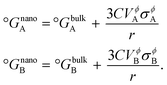
The CALPHAD (CALculation of PHAse Diagrams) methodology18 (ESI S1.1†) is extended to nanoscale systems as explained by Park et al.19 where the total Gibbs free energy of a phase Gϕ,totalm includes the dominant surface energy term, and is given by,| | | Gϕ,totalm = Gϕ,bulkm + ΔGϕ,surfacem, | (1) |
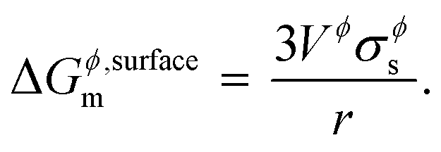
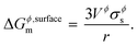
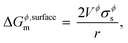
where, Gϕ,bulkm is given by eqn (S2).† According to Gibbs,22 the molar surface Gibbs free energy is given by,| | | ΔGϕ,surfacem = Aϕ,specVϕσϕs, | (2) |
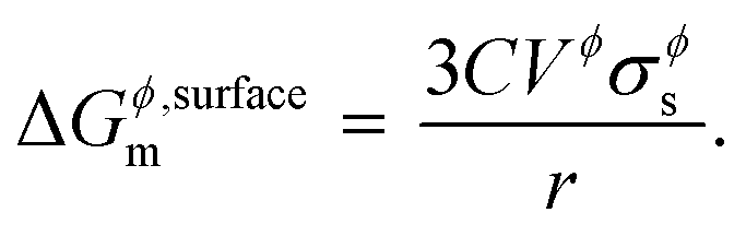
where, Aϕ,spec is the specific area of the phase ϕ given by a ratio of its absolute surface area to absolute volume, Vϕ is its molar volume, and σϕs is the interfacial/surface tension between the phase and its surroundings. In this work, the particles are assumed to be spherical in shape of radius r for reasons explained in the previous section, including the availability of experimental data.20 The specific area of such a phase is given by,| |  | (3) |
By inserting appropriate expressions in the equation above, this methodology can be extended to any geometrical shape, such as thin films or 3D structures. In the work by Eichhammer et al.23 a solid nanowire in contact with a hemispherical alloy nano-particle of different sizes was modeled to calculate its corresponding phase equilibria. As mentioned earlier, for more complicated particle shapes that are multi-facetted, the specific area above (or the surface area to volume ratio) is even higher than that for a sphere. For example in the case of an icosahedron, a regular polyhedron with 20 equilateral triangular faces, the specific area is  .24,25 This is slightly higher than that for a sphere, causing a shift in the phase equilibria in a direction such that the shift in phase equilibria due to spherical particles still remain at the minimum. Fig. S1† shows this effect in the case of the Ge–Si system, which will be discussed in detail in the subsequent section. This makes it more likely that particles form in the spherical shape than any other shape so as to obtain the lowest molar surface Gibbs free energy and total Gibbs free energy. Thus the phase diagrams calculated for spherical particle systems represent the lowest energy and most stable configuration for nano-particles.
Inserting eqn (3) into (eqn (2)) above, we get,
| |  | (4) |
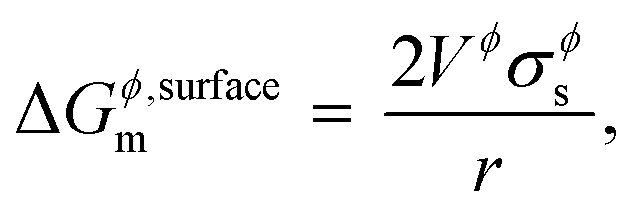
For some systems, information on grain-size distribution is available from experiments, in which case their weighted averages could be used to calculate the surface Gibbs energy. The corresponding Kelvin equation given by,
| |  | (5) |
is most often used in literature,
3,19,26,27 and its incorrectness, as explained by Kaptay in
ref. 1, is mainly due to the fact that the Kelvin equation is derived from substituting inner pressure for outer pressure. A correction factor
C is commonly introduced in the equation above to take into account the effects from shape, surface strain due to non-uniformity, and uncertainty in surface tension measurements,
26 and is estimated to be 1.00 for liquids and 1.05 for solids. Thus,
eqn (4) becomes
| |  | (6) |
The molar volume V of the phase, assuming an ideal solution with no excess volume of mixing, is given by a fractional contribution of each of its pure components,
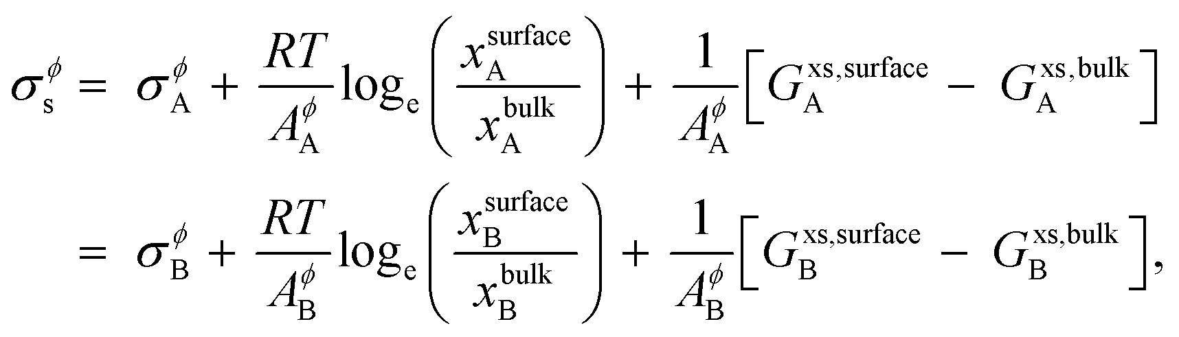
The surface tension of alloy solution phases is calculated for liquids using Butler's model28 that assumes that the surface can be modeled as a single close-packed monolayer. The monolayer layer is treated as an independent thermodynamic phase in equilibrium with the bulk phase. This model has been verified with experimental data,29–33 and according to this model, binary alloy surface tension is given by,
| | 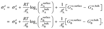 | (8) |
where,
σϕA (
σϕB) is the surface tension of pure component
A (
B) in the phase
ϕ,
R is the gas constant,
T is the temperature,
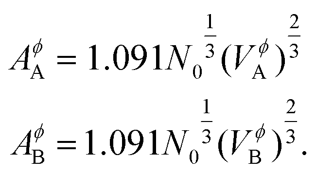
AA (
AB) is the molar surface area of component
A (
B) which is related to molar volumes through Avogadro's number
N0,
| | 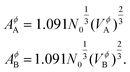 | (9) |
xsurfaceA (
xsurfaceB) and
xbulkA (
xbulkB) are the concentrations of
A (
B) in the surface and bulk phases, respectively.
Gxs,bulkA (
Gxs,bulkB) is the excess Gibbs free energy of A (B) in the bulk phase, similar to eqn (S3),
† and
Gxs,surfaceA (
Gxs,surfaceB) is the partial excess Gibbs free energy of A (B) in the surface and is a function of
T and
xsurfaceA (
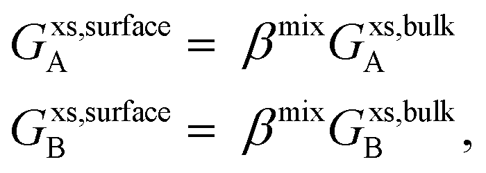
xsurfaceB). According to Yeum's model,
34| | 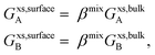 | (10) |
where,
βmix is a parameter corresponding to the ratio of the coordination number in the surface to that of the bulk. Tanaka
et al.30,35,36 showed that
βmix is not surface concentration dependent for many liquid alloys, and that it can be assumed that
βmix is the same as
βpure. Due to surface relaxation and surface atomic rearrangements,
βpure is estimated to be 0.83.
19,29 For solid metals too,
βpure is found to have the same value as liquid metals.
19 Thus, if differences in shape and surface strains as a function of composition are ignored, surface tensions of solid alloys, can be calculated using Butler's model in a similar way as for liquid alloys.
19
Combining Gϕ,bulkm (from eqn (S2) and (S3)†) and ΔGϕ,surfacem (from eqn (6)) in eqn (1), the total Gibbs free energy of a phase Gϕ,totalm consisting of particles of nanoscale dimensions is obtained,
| |  | (11) |
Now, the total Gibbs free energy of this phase can also be defined similar to that of the bulk phase in eqn (S2)† above as,
| |  | (12) |
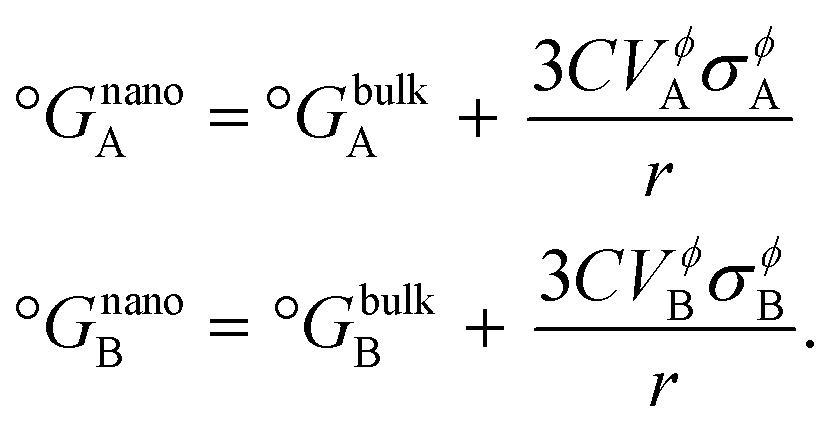
where, for nanoscale systems, the standard Gibbs free energy of pure components is redefined in terms of particle size
r19 using the same spherical particle approximation as discussed earlier, and is given by,
| |  | (13) |
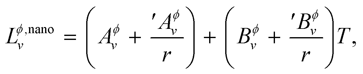
Following the work by Park et al.19 the non-ideal interaction parameter of a phase Lϕ,nanov is not only temperature dependent as for a bulk phase in eqn (S4),† but is now also made size-dependent by expanding it as,
| | 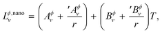 | (14) |
where, ′
Aϕv and ′
Bϕv are also user-defined parameters in addition to
Aϕv and
Bϕv. Using
eqn (17) and (18) in
eqn (15), and then comparing it to
eqn (14), on re-arrangement, it is finally obtained,
| |  | (15) |
This equation is used to solve for the unknown parameters ′Aϕv and ′Bϕv as described in ESI S1.2† on the assessment methodology followed in this work.
2.2. Assessment methodology
In this work, we have used the Thermo-Calc37 package for the calculation of phase diagrams. To calculate a phase diagram, the first step is to determine the bulk Gibbs free energies Gϕ,bulkm (in eqn (S1) and (S2)†) for each phase expected to participate in the bulk equilibrium phase diagram. For the binary systems studied in this work, bulk thermodynamic models have in the past been assessed and developed by various authors. This served as a starting point for the calculation of phase diagrams of nanoscale systems in this work. In cases where bulk models are not available, parameters can be optimized and fitted to either experimental or ab initio data18 using parameter optimization tools implemented in CALPHAD software (PARROT module in Thermo-Calc).
The next step involves the calculation of alloy surface tensions, which are functions of temperature and composition of the components, using Butler's model in eqn (7). This requires temperature-dependent surface tensions and molar volumes of each pure component in the phase for which alloy surface tension is being calculated, and is collected from literature and shown in Table S2.† Then Butler's equations are solved for alloy surface tension as follows: (i) a temperature T and bulk composition xbulkA is selected, (ii) σϕA, σϕB, AϕA, and AϕB are inserted into eqn (7), (iii) using the condition for equilibrium: Gxs,surfaceA = Gxs,surfaceB, eqn (7) is solved by the Newton–Raphson method for σϕs and xsurfaceA (= 1 − xsurfaceB) as functions of temperature and bulk compositions. This procedure is repeated at different temperatures, preferably in the range of stability of the phase, and the resulting data is inserted into eqn (14) to obtain the fitted parameters ′Aϕv and ′Bϕv. In this work, surface tensions of liquid alloys in all three binary systems studied here are calculated using the above model, whereas in only the Ge–Si system, surface tension of the solid (diamond) phase is also calculated as it is the only system for which the ground state phase of both the pure element constituents Ge and Si exhibit continuous solid solubility across the entire composition space.
2.3. DFT calculations of surface energy
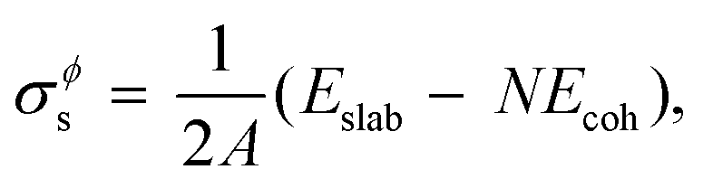
As stated in the Introduction section of the main text, no compound phases exist in the bulk equilibria of the Au–Si and Ge–Si systems (metastable phases are not considered in this work). However, the Al–Cu bulk phase diagram has numerous intermetallic phases in equilibrium.38,39 In this work we have followed the methodology presented by Kroupa et al. in ref. 40 by calculating the surface energy of one such compound Al2Cu from ab initio DFT calculations,21 which is then used in the CALPHAD model. A slab model with two surfaces of the same type is created by inserting a vacuum. The surface tension σϕs of such a model is then obtained by subtracting the cohesive energy of the bulk structure Ecoh from the energy of the slab structure Eslab,| | 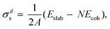 | (16) |
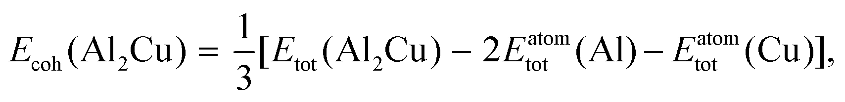
where, N is the number of atoms in the slab structure, and A is the area of the surface being considered. Cohesive energy is calculated using the following equation,| |  | (17) |
where, Etot(Al2Cu) represents the total energy per formula unit of Al2Cu, and Eatomtot(Al) and Eatomtot(Cu) are the total energies of Al and Cu, respectively. The surface tension is then used to calculate the surface energy using the spherical particle approximation in a similar way as discussed in the main text (see eqn (5)),| |  | (18) |
The surface energies of the (100), (110), and (111) planes of Al2Cu are calculated, and the minimum is included in the model of the Al–Cu system. This method is advantageous as, in principle, the surface energy contribution of all elements, compounds, and metastable phases can be calculated. The Al–Cu system is complex with many intermetallic phases participating in phase equilibria, so a logical extension of our current work is to perform surface energy calculations for all such structures and compare the impacts on the model predictions. It should be noted here that the larger the number of phases for which surface energies are calculated and included in the thermodynamic model, larger will be the difference in phase diagrams (melting points, reaction temperatures, etc.) between the nano and bulk systems.
The Al2Cu compound is of tetragonal tI12 symmetry with space group I4/mcm (no. 140). The unit cell has the dimensions a = 6.067 Å and c = 4.877 Å.41 DFT calculations were performed using the Vienna Ab-initio Simulation Package (VASP),42–45 and ion–electron interactions were described using the Projector Augmented Wave (PAW) method.46–48 The 3s22p1 orbitals of Al and 3d104s1 orbitals of Cu were treated as valence states to generate the PAW potentials. Non spin-polarized Local Density Approximation (LDA)49 was used to approximate the exchange–correlation functional. The cutoff energy of plane wave basis was set to 500 eV, and integrations over the first Brillouin zone were made using a k-point grid set of 8 × 8 × 10 (and scaled appropriately for slab structures), generated according to the Γ-centered Monkhorst–Pack scheme.50 Unit cell parameters and atomic positions were relaxed based on an energy convergence criteria of 10−4 eV per atom, and a final static calculation was performed for an accurate total energy.
3. Results and discussion
3.1. Au–Si
There are very few experimental results that allow a direct comparison with theoretical results, and the work by Kim et al.20 on the Au–Si system is one of the few. In their study, spherical Au nano-particles ≈35 nm in diameter were continuously exposed to disilane (Si2H6) gas, and imaged with a transmission electron microscope. It was observed that with time, solid Au shrinks and the added Si forms a liquid AuSi shell on its surface, which grows until no solid Au remains. Thus, the transition from the two-phase sol-Au + liq-AuSi region of the phase diagram to the single-phase liq-AuSi is recorded. It was concluded that at 500–525 °C the liquidus is shifted in composition by Δx = 3.5 at% more Au-rich, and that the transition temperature is lowered by ≈240° C. The use of sphere-shaped particles in this study, and the fact that the above experimental data was used to make a direct correlation to a shift in the liquidus line, made the Au–Si system a perfect candidate to verify the spherical particle approximation employed in the thermodynamic models shown in the Method section.
Table S2† shows surface tensions and molar volumes of Au and Si, in the liquid and solid phases, as functions of temperature that are employed in this work. These functions lead to calculated melting points of Au and Si shown in Fig. S2 and S3,† respectively, along with experimental data from literature which they are in fair agreement with. As expected from eqn (17), they vary inversely as a function of particle radius r. The surface tension data of liquid Si from literature shows considerable scatter as discussed in ref. 51, and ranges anywhere between the so-called “high” and “low” values of σ = 0.86 J m−2 and σ = 0.74 J m−2, respectively. The resulting value is debated to depend on the measurement method (sessile drop, large drop, levitation techniques, oscillating drop method), the crucible/substrate material, and oxygen contamination.52 In this work we have chosen the “low” value from ref. 53, i.e. σLSi = 0.732 − 8.6 × 10⁻⁵(T − 1687.15), because when combined with surface tension of solid Si: σSSi = 1.510 − 1.589 × 10⁻⁴(T − 298.2),54 the resulting melting points of Si lie within the upper and lower limits defined by Couchman et al.55 Results from the study on isolated Si particles of sizes ≤6 nm by Goldstein ref. 56 show a much more significant drop in melting points. Due to the previously mentioned size limitations in the CALPHAD model, the applicability of the spherical particle approximation in this current method is limited to radius exceeding 5 nm. cannot be neglected as in this study. Thus, the applicability of the spherical particle approximation in this method is limited to radius exceeding 5 nm. Curve (a) in Fig. S3† is calculated using surface tension data of liquid and solid Si from ref. 57 and 58, respectively, and is in worse agreement with literature data. Discrepancies in melting temperatures can be attributed to several reasons: due to the fact that experimental melting temperatures are not defined by the equality of Gibbs energy of the solid and liquid phases; nanoparticles are prone to defects and impurities especially due to their relatively large surface areas; although phase-field theory has its own limitations, it has been demonstrated using phase-field approach59,60 that surface melting can begin at lower temperatures than complete melting and that complete melting occurs when the interface between the surface melt and solid core loses its stability as the surface melt propagates towards the center, which is determined by local equilibrium conditions at the interface; due to kinetics and thermal fluctuations, melting may start when the kinetic nucleation criterion is satisfied.
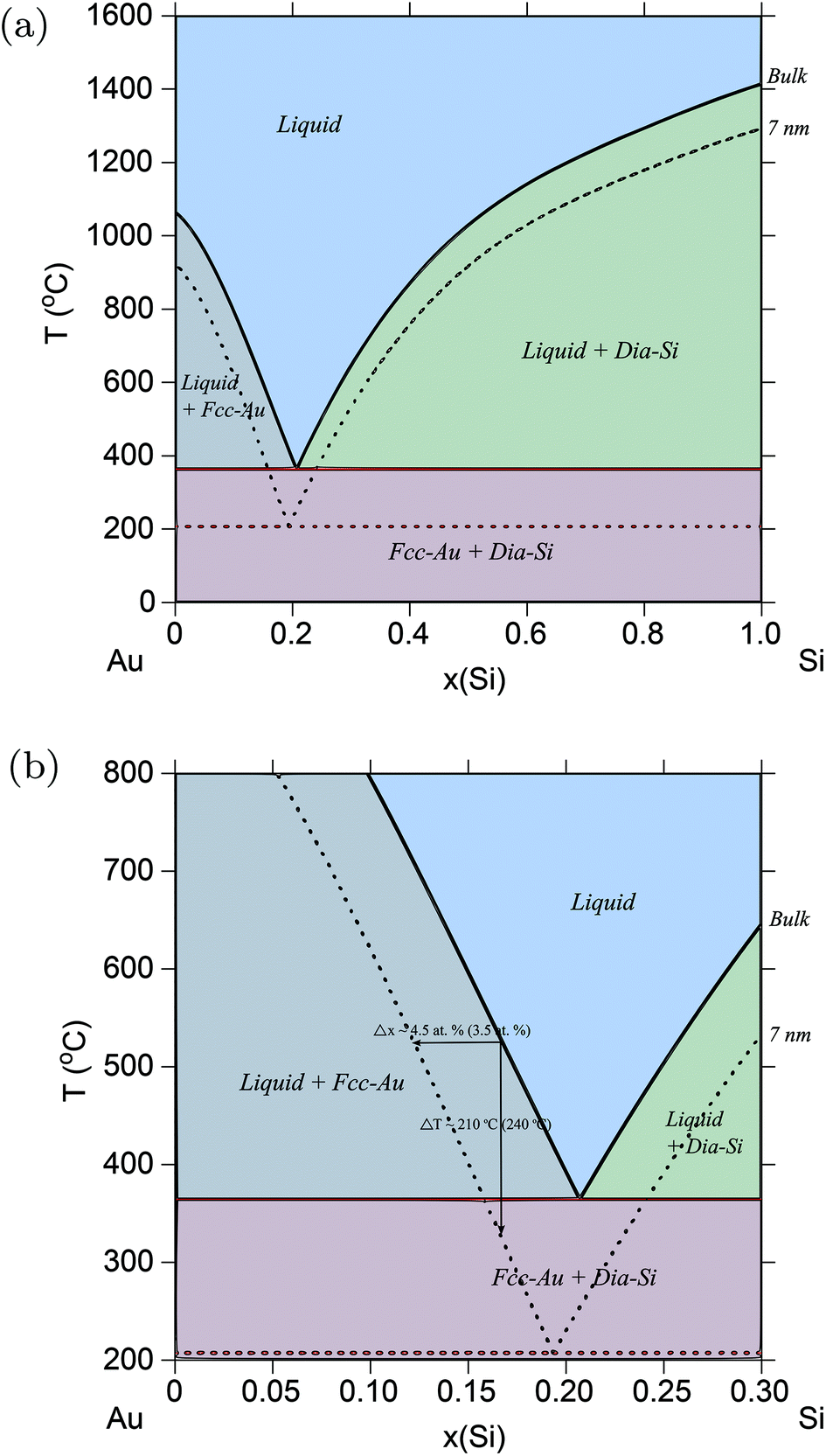
Following the methodology explained in the Method section, we first start with bulk thermodynamic data of Au–Si which is obtained from the work by Meng et al.61 His model was optimized with measured data on mixing enthalpies of the liquid phase and activities of Au and Si. Then, using the surface tension and volumetric data of Au and Si, Butler's equations are solved to calculate alloy surface tension of the liquid phase of Au–Si as a function of temperature and composition. Parameters ′Aϕv and ′Bϕv are then fitted to this data using eqn (15). Increasing the order parameters v was found to have no significant effect on the phase diagrams, and thus its maximum value was kept the same between nano and bulk systems. Resulting non-ideal interaction parameters, combined with bulk parameters, are shown in Table S3† along with the modified standard Gibbs energies of pure components. This completes the thermodynamic model for nano-sized particles, and the resulting phase diagrams can be calculated for different particle sizes by changing r.
Fig. 1a shows the calculated Au–Si phase diagram at r = 7 nm. Fig. 1b shows the same phase diagram, but now plotted to compare with the experimental data from ref. 20. The amount of shift of the liquidus solubility line, and the drop in transition temperature agrees very well with the predicted amounts in ref. 20. As discussed earlier, the use of spherical particles in ref. 20 serves as a direct validation of the spherical particle model used in this study to calculate surface energies. Table 1 shows the drop in eutectic temperatures and its compositional shifts in the Au–Si system as a function of particle size.
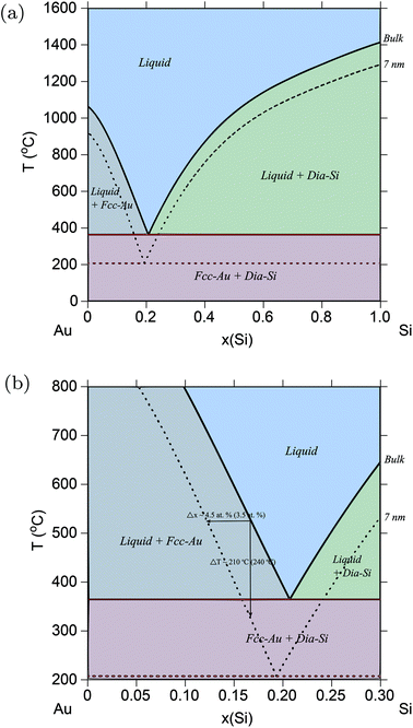 |
| | Fig. 1 (Color online) Au–Si phase diagram. (a) Phase diagram of the Au–Si alloy system calculated for particles of radius, r = 7 nm, and compared with the bulk phase diagram from ref. 61. (b) Part of Au–Si phase diagram showing the amounts of shift in solubility lines which agrees well with experimental results from ref. 20 shown in parentheses. | |
Table 1 Change in points on the phase diagram for particles from bulk to nanoscale dimensions. Au–Si: temperature and composition of the eutectic point – Liq → fcc-Au + dia-Si, Ge–Si: peak temperature of the miscibility gap in the diamond phase, and Al–Cu: temperature and composition of the eutectic point – Liq → fcc-Al + Al2Cu
| Radius (nm) |
Au–Si: Liq → fcc-Au + dia-Si |
Ge–Si: peak miscibility gap |
Al–Cu: Liq → fcc-Al + Al2Cu |
|
x(Si) (at%) |
T (°C) |
T (K) |
x(Cu) (at%) |
T (K) |
| Bulk |
20.6 |
364.2 |
226.5 |
17.5 |
821 |
| 90 |
20.6 |
353.1 |
218.6 |
18.2 |
812.5 |
| 65 |
20.6 |
348.8 |
215.6 |
18.4 |
810 |
| 45 |
20.5 |
341.8 |
210.5 |
18.7 |
805 |
| 32 |
20.5 |
332.6 |
204.2 |
19.3 |
799 |
| 22 |
20.3 |
317.7 |
193.7 |
20.2 |
787.5 |
| 14 |
20.1 |
289.9 |
174.3 |
21.8 |
767.5 |
| 10 |
19.8 |
257.9 |
152.1 |
23.5 |
744 |
| 7 |
19.4 |
207.4 |
117.5 |
25.1 |
717 |
| 5 |
18.6 |
134.2 |
68.1 |
25.8 |
695 |
3.2. Ge–Si
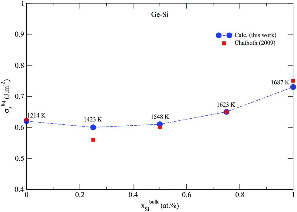
Semiconductors based on GeSi are used in electronic devices for a wide variety of applications, making it of great industrial and technological importance. The above validated model is applied to the Ge–Si system following the same methodology, but this time, alloy surface tension of the solid diamond phase is also calculated in addition to that of the liquid phase. This is possible because the solid diamond phase in the Ge–Si system exhibits continuous solid solubility between its pure components Ge and Si up to very high temperatures in the order of 1200 K, as shown in Fig. 2a. This phase also exhibits a low-temperature symmetrical miscibility gap with its highest point at ≈226.5 K. The bulk thermodynamic data of the liquid and diamond phases is extracted from ref. 63 and 64, respectively. Fig. 3 shows the calculated surface tensions of the liquid phase at various compositions and temperatures, and agrees very well with experimental data on Si and Ge melts from ref. 65. Complete thermodynamic functions of the model are listed in Table S3.† The functions for Ge lead to melting points shown in Fig. S4† compared with experimental data on Ge nanocrystals. The calculated phase diagram at particle radius r = 22 nm is shown in Fig. 2b, and as expected, equilibrium lines are lowered in temperature from their positions in the bulk phase diagram. At the suggested lowest particle size of r = 5 nm for the nano-CALPHAD method, the peak temperature of the solid phase miscibility gap is reduced to 68.1 K as shown in Fig. 2b. Table 1 lists the calculated peak temperatures of the miscibility gap. The depression of the miscibility gap at small particle sizes due to larger contributions of surface energy terms could have significant implications for engineering alloy design and fabrication which rely on phase diagram to tune thermodynamic, electrical, and transport properties.
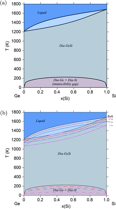 |
| | Fig. 2 (Color online) Ge–Si phase diagram. (a) Bulk Ge–Si phase diagram calculated using data from ref. 62–64. (b) Phase diagram of the Ge–Si alloy system calculated for varying radii particles, and compared with the bulk phase diagram. With decreasing particle radii, the peak temperature of the miscibility gap decreases from ≈226 K for bulk particles to ≈68 K for particles of radii, r = 5 nm. | |
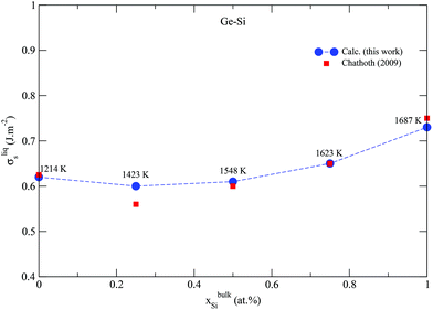 |
| | Fig. 3 (Color online) Calculated surface tension of the liquid phase in the Ge–Si system compared with experimental data from ref. 65. Dashed line only serves as guide to the eye. | |
3.3. Al–Cu
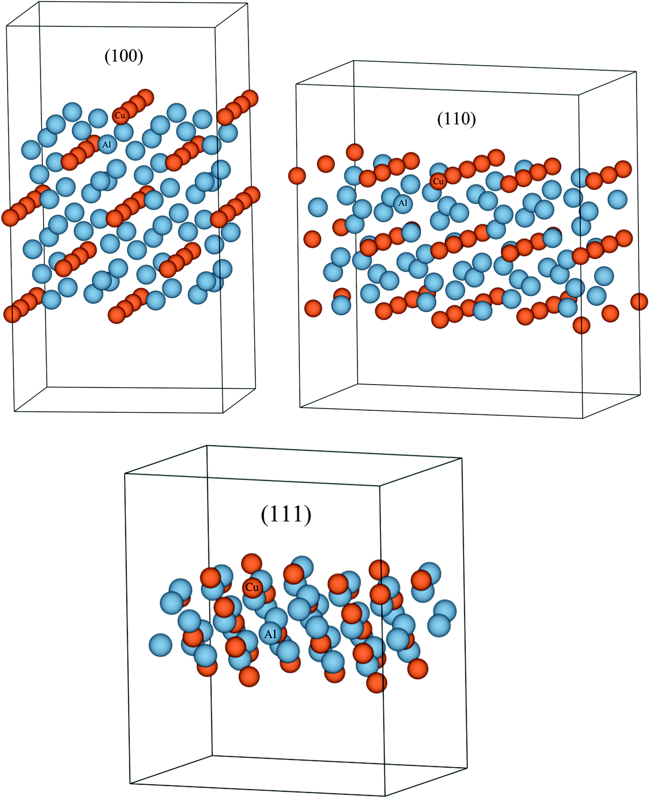
The Al–Cu system is different from the Au–Si and Ge–Si systems in that there are a number of intermetallic compounds, totaling to 13, both stoichiometric and non-stoichiometric, that participate in the equilibrium phase diagram,38,39 as shown in Fig. 4a. In principle, the thermodynamic model of Al–Cu must include surface energies of all these compounds in addition to those of the liquid and room-temperature solid phases. Since such data is largely unavailable for most systems from literature, one can resort to DFT to calculate the surface tension of each phase. However, calculating the surface tension of different planes in each of the 13 compounds is computationally expensive. For the purpose of demonstration, in this work we have calculated the surface energy of only one such compound Al2Cu from DFT, and included that in the thermodynamic model to calculate the phase diagram of Al–Cu.
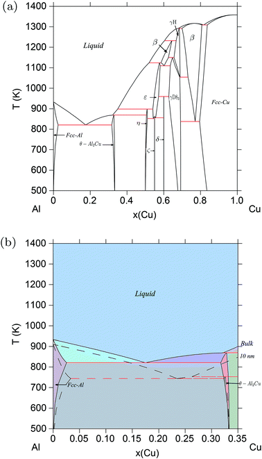 |
| | Fig. 4 (Color online) Al–Cu phase diagram. (a) Bulk Al–Cu phase diagram according to refs. 39, 38. (b) Phase diagram of the Al–Cu alloy system calculated for particles of radius r = 10 nm, compared with the bulk phase diagram at Al-rich/Cu-poor compositions. The eutectic temperature drops from ≈821 K for bulk particles to ≈695 K for particles of radii, r = 5 nm. | |
Details of the calculation methods used, and structural information about the Al2Cu compound are mentioned in ESI S1.3.† Its unit cell is shown in Fig. S5.† The calculated structural and cohesive energies of the compound, along with those of Al and Cu, are compared with experimental data in Table S4.† These results are in accordance with the observation of under-estimation of lattice constants and over-estimation of cohesive energies by the LDA approximation to the exchange–correlation functional.66 Slab models were created for the (100), (110), and (111) surfaces as shown in Fig. 5. Both the height of the vacuum, and number of atomic layers were varied in each model so as to obtain converged surface tension values. Table 2 shows the resulting surface tensions of each surface as a function of vacuum height and number of atomic layers calculated using eqn (S5).† Since the surface tension of the (111) plane is the lowest, its surface energy calculated using eqn (S7)† is inserted into the thermodynamic model. Thermodynamic functions for this phase, along with non-ideal interaction parameters computed for the liquid phase, and standard Gibbs energies of Al and Cu are listed in Table S3.† Melting points of Al and Cu calculated using these functions as a function of particle size agree with experimental data on synthesized nano-particles as shown in Fig. S6 and S7,† respectively, and so does the liquid phase surface tensions calculated using Butler's equations at T = 1375 K as shown in Fig. S8.† The good agreement of the model predictions and experimental data suggest that even for complex systems with many intermetallics such as Al–Cu, rigorous calculations of surface and phase data for a single or a limited number of critical compositions may be sufficient to eliminate the need for wide-ranging calculations for all intermetallics. The Al–Cu phase diagram calculated at r = 10 nm is shown in Fig. 4b. Only Al-rich compositions are shown in this figure as the surface tension of only one of several intermetallic compounds, Al2Cu, is calculated in this work. Table 1 shows the drop in temperature and shift in composition of the eutectic reaction: Liq → fcc-Al + Al2Cu as particle sizes are decreased.
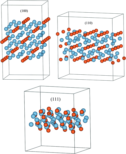 |
| | Fig. 5 (Color online) Slab models created for the calculation of surface energies of the (100), (110), and (111) planes in the Al2Cu compound. These surface energies can then be used to calculate the surface energy contribution to the total Gibbs free energy of this phase which will lead to the estimation of the change in phase stability of this compound in the phase diagram as a function of particle radii. Since the surface energy can theoretically be calculated for any compound using DFT, this method can be applied to all the phases in a system including equilibrium, metastable and unstable phases. | |
Table 2 Converged surface tension values of different planes in the Al2Cu intermetallic compound calculated from DFT using the LDA approximation
| Plane |
Surface tension, 
|
| meV Å−2 |
J m−2 |
| (100) |
0.079 |
1.275 |
| (110) |
0.099 |
1.586 |
| (111) |
0.077 |
1.227 |
4. Conclusions and outlook
In this work, by calculating phase diagrams at varying particle radii, we have shown the considerable changes in equilibrium thermodynamics resulting from decreasing particle sizes to nanoscale dimensions. At these particle sizes, the surface to volume ratio is drastically increased, and so is the contribution of surface energy to the Gibbs free energies of the phases. This dominant surface energy term is calculated using the spherical particle approximation that assumes particles to be spherical in shape. In a similar way, this methodology can be extended to non-spherical particles using a non-ideality factor in the Gibbs surface energy term.
The Au–Si system was first chosen as it is one of the few systems for which experimental data that estimates shift in equilibrium lines for spherical nano-particles was available. This allowed for a direct verification of the surface energy models that assume sphere-shaped particles, and the resulting phase diagram was in good agreement. Phase diagrams of Ge–Si particles were computed in a similar way, and a considerable depression of the miscibility gap was noted. This is vital when, for example, alloys are designed to achieve compositions that do not lie in the miscibility gap to achieve a desired band gap value. Finally, DFT was used to compute the surface energy of one of the many intermetallic compounds in the Al–Cu system. This was then added to its thermodynamic model, and a drop in the eutectic temperature in its phase diagram was tabulated.
To conclude, due to surfaces (and interfaces) materials can have considerably different thermodynamic and phase stability behavior from bulk systems, and as transistor and devices continue to be scaled down in sizes, the study of their phase stability becomes necessary. This is critical not only for designing semiconductor alloys and compounds, but also for tuning their electrical, thermodynamic, and transport properties in order to achieve optimum device performance.
Acknowledgements
The authors thank Intel Corporation for the specific project definition, and the internship opportunity. The Materials and Process Simulation Center (MSC) at Caltech (with funding from DARPA W31P4Q-13-1-0010), and the Chemical Engineering Cluster at Texas A&M University are acknowledged for providing computing resources useful in conducting the research reported in this work.
Notes and references
- G. Kaptay, J. Mater. Sci., 2012, 47, 8320–8335 CrossRef CAS.
- W. A. Jesser, R. Z. Shneck and W. W. Gile, Phys. Rev. B: Condens. Matter, 2004, 69, 144121 CrossRef.
- J. Lee, J. Lee, T. Tanaka, H. Mori and K. Penttilä, JOM, 2005, 57, 56–59 CrossRef CAS PubMed.
- N. Braidy, G. R. Purdy and G. A. Botton, Acta Mater., 2008, 56, 5972–5983 CrossRef CAS PubMed.
- J. Lee, J. Lee, T. Tanaka and H. Mori, Nanotechnology, 2009, 20, 475706 CrossRef PubMed.
- C. Zou, Y. Gao, B. Yang and Q. Zhai, J. Mater. Sci.: Mater. Electron., 2010, 21, 868–874 CrossRef CAS.
- T. T. Bao, Y. Kim, J. Lee and J.-G. Lee, Mater. Trans., 2010, 51, 2145–2149 CrossRef CAS.
- J.-G. Lee and H. Mori, Eur. Phys. J. D, 2005, 34, 227–230 CrossRef CAS.
- M. Wautelet, J. Phys. D: Appl. Phys., 1991, 24, 343–346 CrossRef CAS.
- J.-A. Yan, L. Yang and M. Y. Chou, Phys. Rev. B: Condens. Matter, 2007, 76, 115319 CrossRef.
- H. Naganuma, K. Sato and Y. Hirotsu, J. Magn. Magn. Mater., 2007, 310, 2356–2358 CrossRef CAS PubMed.
-
M. Quinten, Optical Properties of Nanoparticle Systems: Mie and Beyond, Wiley-VCH, 2011 Search PubMed.
- B. F. G. Johnson, Top. Catal., 2003, 24, 147–159 CrossRef CAS.
- M. Takagi, J. Phys. Soc. Jpn., 1954, 9, 359–363 CrossRef.
- C. L. Chen, J.-G. Lee, K. Arakawa and H. Mori, Appl. Phys. Lett., 2011, 99, 013108 CrossRef PubMed.
- W. A. Jesser and C. T. Schamp, Phys. Status Solidi C, 2008, 5, 539–544 CrossRef CAS PubMed.
- G. E. Moore, Electronics, 1965, 38 Search PubMed.
- N. Saunders and A. P. Miodownik, Pergamon Mater. Ser., 1998, 91–109 Search PubMed.
- J. Park and J. Lee, CALPHAD: Comput. Coupling Phase Diagrams Thermochem., 2008, 32, 135–141 CrossRef CAS PubMed.
- B. J. Kim, J. Tersoff, C.-Y. Wen, M. C. Reuter, E. A. Stach and F. M. Ross, Phys. Rev. Lett., 2009, 103, 155701 CrossRef CAS.
-
R. M. Martin, Electronic Structure, Cambridge University Press, Cambridge, England, 2004 Search PubMed.
- J. W. Gibbs, Trans Conn Acad Arts Sci., 1875–1878, 3(108), 343 Search PubMed.
- Y. Eichhammer, M. Heyns and N. Moelans, CALPHAD: Comput. Coupling Phase Diagrams Thermochem., 2011, 35, 173–182 CrossRef CAS PubMed.
-
http://www.math.rutgers.edu/erowland/polyhedra.html
.
-
http://wordpress.mrreid.org/2011/10/20/spherical-ice-cubes-and-surface-area-to-volume-ratio/
.
- J. Lee, T. Tanaka, J. G. Lee and H. Mori, CALPHAD: Comput. Coupling Phase Diagrams Thermochem., 2007, 31, 105–111 CrossRef CAS PubMed.
- T. Ivas, A. N. Grundy, E. Povoden-Karadeniz and L. J. Gauckler, CALPHAD: Comput. Coupling Phase Diagrams Thermochem., 2012, 36, 57–64 CrossRef CAS PubMed.
- J. A. V. Butler, Proc. R. Soc. London, Ser. A, 1932, 135, 348–375 CrossRef CAS.
- T. Tanaka, K. Hack, T. Iida and S. Hara, Z. Metallkd., 1996, 87, 380–389 CAS.
- T. Tanaka, K. Hack and S. Hara, CALPHAD: Comput. Coupling Phase Diagrams Thermochem., 2000, 24, 465–474 CrossRef CAS.
- Z. Moser, W. Gasior and J. Pstrus, J. Phase Equilib., 2001, 22, 254–258 CrossRef CAS.
- J. Lee, W. Shimoda and T. Tanaka, Mater. Trans., 2004, 45, 2864–2870 CrossRef CAS.
- R. Picha, J. Vrestal and A. Kroupa, CALPHAD: Comput. Coupling Phase Diagrams Thermochem., 2004, 28, 141–146 CrossRef CAS PubMed.
- K. S. Yeum, R. Speiser and D. R. Poirier, Metall. Trans. B, 1989, 20, 693–703 CrossRef.
- T. Tanaka and S. Hara, Z. Metallkd., 2001, 92, 467–472 CAS.
- T. Tanaka and S. Hara, Z. Metallkd., 2001, 92, 1236–1241 CAS.
- J.-O. Andersson, T. Helander, L. Höglund, P. Shi and B. Sundman, CALPHAD: Comput. Coupling Phase Diagrams Thermochem., 2002, 26, 273–312 CrossRef CAS.
-
N. Saunders, Al-Cu system, in COST-507: Thermochemical Database For light Metal Alloys, ed. I. Ansara, A. T. Dinsdale and M. H. Rand, European Communities, Luxemburg, 1998, pp. 28–33 Search PubMed.
- V. T. Witusiewicz, U. Hecht, S. G. Fries and S. Rex, J. Alloys Compd., 2004, 385, 133–143 CAS.
-
A. Kroupa, T. Kana and A. Zemanova, in Proceedings of Nanocon 2012 conference, Brno, Czech Republic, 2012.
- A. Meetsma, J. L. De Boer and S. Van Smaalen, J. Solid State Chem., 1989, 83, 370–372 CrossRef CAS.
- G. Kresse and J. Hafner, Phys. Rev. B: Condens. Matter, 1993, 47, 558–561 CrossRef CAS.
- G. Kresse and J. Hafner, Phys. Rev. B: Condens. Matter, 1994, 49, 14251–14269 CrossRef CAS.
- G. Kresse and J. Furthmüller, Comput. Mater. Sci., 1996, 6, 15–50 CrossRef CAS.
- G. Kresse and J. Furthmüller, Phys. Rev. B: Condens. Matter, 1996, 54, 11169–11186 CrossRef CAS.
- P. E. Blöchl, Phys. Rev. B: Condens. Matter, 1994, 50, 17953–17979 CrossRef.
- G. Kresse and D. Joubert, Phys. Rev. B: Condens. Matter, 1999, 59, 1758–1775 CrossRef CAS.
- O. Bengone, M. Alouani, P. Blöchl and J. Hugel, Phys. Rev. B: Condens. Matter, 2000, 62, 16392–16401 CrossRef CAS.
- J. P. Perdew and A. Zunger, Phys. Rev. B: Condens. Matter, 1981, 23, 5048–5079 CrossRef CAS.
- H. J. Monkhorst and J. D. Pack, Phys. Rev. B: Condens. Matter, 1976, 13, 5188–5192 CrossRef.
- N. Eustathopoulos and B. Drevet, J. Cryst. Growth, 2013, 371, 77–83 CrossRef CAS PubMed.
- B. J. Keene, SIA Surf. Interface Anal., 1987, 10, 367–383 CrossRef CAS PubMed.
- F. Millot, V. Sarou-Kanian, J. C. Rifflet and B. Vinet, Mater. Sci. Eng., A, 2008, 495, 8–13 CrossRef PubMed.
- R. J. Jaccodine, J. Electrochem. Soc., 1963, 110, 524–527 CrossRef CAS PubMed.
- P. R. Couchman and W. A. Jesser, Nature, 1977, 269, 481–483 CrossRef CAS PubMed.
- A. N. Goldstein, Appl. Phys. A: Mater. Sci. Process., 1995, 62, 33–37 CrossRef.
-
T. Iida and R. I. L. Guthrie, The Physical Properties of Liquid Metals, Oxford Science Publications, 1993 Search PubMed.
- L. Z. Mezey and J. Giber, Jpn. J. App. Phys., 1982, 21(11), 1569–1571 CrossRef CAS.
- V. I. Levitas and K. Samani, Nat. Commun., 2011, 2(284), 1–6 Search PubMed.
- V. I. Levitas and K. Samani, Phys. Rev. B: Condens. Matter, 2014, 89, 075427 CrossRef.
- F. G. Meng, H. S. Liu, L. B. Liu and Z. P. Jin, J. Alloys Compd., 2007, 431, 292–297 CrossRef CAS PubMed.
- A. T. Dinsdale, CALPHAD: Comput. Coupling Phase Diagrams Thermochem., 1991, 15, 317–425 CrossRef CAS.
- R. W. Olesinski and G. J. Abbaschian, Bull. Alloy Phase Diagrams, 1984, 5, 180–183 CrossRef CAS.
- Y.-B. Kang, C. Aliravci, P. J. Spencer, G. Eriksson, C. D. Fuerst, P. Chartrand and A. D. Pelton, JOM, 2009, 61(4), 75–82 CrossRef CAS PubMed.
- S. M. Chathoth, B. Damaschke, K. Samwer and S. Schneider, J. Appl. Phys., 2009, 106, 103524 CrossRef PubMed.
- R. O. Jones and O. Gunnarsson, Rev. Mod. Phys., 1989, 61, 689–746 CrossRef CAS.
Footnote |
| † Electronic supplementary information (ESI) available. See DOI: 10.1039/c5nr01535a |
|
| This journal is © The Royal Society of Chemistry 2015 |
Click here to see how this site uses Cookies. View our privacy policy here. 
 Open Access Article
 This Open Access Article is licensed under a Creative Commons Attribution-Non Commercial 3.0 Unported Licence
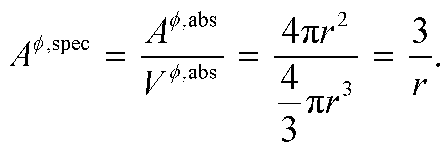
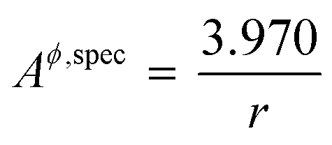 .24,25 This is slightly higher than that for a sphere, causing a shift in the phase equilibria in a direction such that the shift in phase equilibria due to spherical particles still remain at the minimum. Fig. S1† shows this effect in the case of the Ge–Si system, which will be discussed in detail in the subsequent section. This makes it more likely that particles form in the spherical shape than any other shape so as to obtain the lowest molar surface Gibbs free energy and total Gibbs free energy. Thus the phase diagrams calculated for spherical particle systems represent the lowest energy and most stable configuration for nano-particles.