MetDFBA: incorporating time-resolved metabolomics measurements into dynamic flux balance analysis

Abstract

Understanding cellular adaptation to environmental changes is one of the major challenges in systems biology. To understand how cellular systems react towards perturbations of their steady state, the metabolic dynamics have to be described. Dynamic properties can be studied with kinetic models but development of such models is hampered by limited in vivo information, especially kinetic parameters. Therefore, there is a need for mathematical frameworks that use a minimal amount of kinetic information. One of these frameworks is dynamic flux balance analysis (DFBA), a method based on the assumption that cellular metabolism has evolved towards optimal changes to perturbations. However, DFBA has some limitations. It is less suitable for larger systems because of the high number of parameters to estimate and the computational complexity. In this paper, we propose MetDFBA, a modification of DFBA, that incorporates measured time series of both intracellular and extracellular metabolite concentrations, in order to reduce both the number of parameters to estimate and the computational complexity. MetDFBA can be used to estimate dynamic flux profiles and, in addition, test hypotheses about metabolic regulation. In a first case study, we demonstrate the validity of our method by comparing our results to flux estimations based on dynamic ¹³C MFA measurements, which we considered as experimental reference. For these estimations time-resolved metabolomics data from a feast-famine experiment with Penicillium chrysogenum was used. In a second case study, we used time-resolved metabolomics data from glucose pulse experiments during aerobic growth of Saccharomyces cerevisiae to test various metabolic objectives.

---

1 Introduction

Organisms are capable of adapting to changing environmental conditions while maintaining essential functions for survival.^1,2 The consequences of these metabolic adaptations are important to study from an economic perspective but can also play crucial roles in health and disease. A well-known example of such a consequence from biotechnology, is the loss of biomass or product formation due to changes in substrate availability during fermentation processes.³ Examples of changing conditions related to health and disease in human include changes in diet or drug.^4,5 Understanding the principles of adaptation is therefore one of the major challenges in systems biology.^6–9

One manifestation of adaptation on the molecular level is the alteration of fluxes in metabolic networks. This occurs when the availability of substrates changes, which results in changes in fluxes in the affected metabolic pathways.^1,10 The (change in) flux can provide important information about cellular physiology, product yield, and response mechanisms to perturbations. Unfortunately, intracellular fluxes cannot be measured directly but have to be estimated from concentration measurements.^11,12 Various experimental and associated computational methods have been developed to estimate dynamic fluxes through metabolic networks including kinetic models,¹³¹³C-metabolic flux analysis (MFA),^14–16 and dynamic flux balance analysis (DFBA).^17,18 The development of kinetic models is hampered by limited availability and accuracy of information about condition-specific (in vivo) kinetic parameters,¹⁹¹³C MFA is expensive and tracer availability is limited.²⁰

Flux balance analysis (FBA) is a constraint-based modelling approach to determine fluxes in steady state. Mass balance constraints imposed by the stoichiometry of the metabolic network define an under-determined system of linear equations because the network contains more reactions than metabolites. To reduce the solution space, additional constraints on the upper and lower bounds of the fluxes, also called capacity constraints, are imposed. The linear system is solved as an optimization problem by determining the fluxes that minimize a pre-specified mathematically described objective function.²¹ This objective function defines the phenotype (e.g., maximum growth yield or energetic efficiency) in the form of a biological objective such as biomass production. The objective function quantifies the relative contribution of each reaction to the phenotype.^17,22 It has been proposed in the literature that there are conditions for which the optimality principles cannot be described by a single objective, but by a combination of multiple objectives.²³

DFBA, developed by Mahadevan and co-workers,¹⁸ is a non-steady state extension of FBA that accounts for dynamic changes in the cellular metabolism as introduced, for example, after a perturbation. Although FBA could be used for a perturbed system to determine fluxes for the different steady state conditions, this would not describe the transient behavior after a perturbation. DFBA estimates the transient behavior of the fluxes after a perturbation by optimizing the objective function over a time interval of interest. The objective function is subjected to capacity constraints and dynamic mass balance constraints, formulated as differential equations, which specify the change in metabolite concentrations as a function of fluxes, biomass and other available (kinetic) parameters. If available, constraints that specify the maximum change rate of the fluxes at any moment in time can be added. By specifying the stoichiometry, the initial concentrations, biomass and constraints, the fluxes and metabolite concentrations as function of time are calculated for the specified time interval.

In contrast to FBA where the change in metabolite concentration is zero and only the fluxes are unknown, DFBA also needs to estimate the change (derivatives) of the metabolite concentrations as a function of time given the initial conditions. This results in a system with even more unknown parameters which is solved as a dynamic optimization problem by parameterizing the dynamic equations through the use of orthogonal collocation on finite elements.¹⁸ This makes the approach less suitable for larger metabolic networks or for longer-term extracellular dynamics.

Classical DFBA is used to estimate dynamic flux profiles when it is known which objective drives an organism under changing conditions, for example a diauxic shift.¹⁸ Due to the large number of parameters to estimate, it is only used for small systems, mostly describing the flux between extracellular metabolites. In this paper, we describe a new approach that reduces both the computational complexity and the number of parameters to estimate in DFBA. We discuss two applications of this approach, that were hampered by the computational burden of classical DFBA. A first application is the estimation of dynamic flux profiles for larger systems, describing both internal and external fluxes over time after a perturbation, given the objective driving the organism under this particular perturbation. A second application is the evaluation of objective functions driving the transient cellular behavior after perturbations.

Metabolite concentration profiles can directly be measured through, for example, chromatography (liquid or gas) combined with mass spectrometry (LC/GC-MS). From these profiles the changes in concentrations over time can be easily calculated. Hence, instead of estimating time derivatives and metabolite concentrations in DFBA, these can be derived from experimental data. Unfortunately, DFBA cannot incorporate measured concentration profiles. Therefore, we developed a new approach (MetDFBA) which directly uses derivatives calculated from the measured concentration profiles, which are substituted in the mass balance equation leading to a system of linear equations. This approach largely reduces the computational burden of DFBA. The reduced complexity and the smaller number of unknowns makes this framework especially suitable for larger systems.²⁴ In this paper we present our method (MetDFBA) and underlying mathematical framework to determine flux changes after perturbation of a biological system. We first demonstrate the validity of our method by comparing our results to flux estimations based on dynamic ¹³C experiments, which we consider as a experimental reference. For these estimations time-resolved metabolomics data from a feast-famine experiment with Penicillium chrysogenum was used. We only used the metabolite concentration measurements to estimate fluxes based on a single objective function. Subsequently, we compared our flux estimations to ¹³C MFA estimates from the ¹³C mass isotopomer measurements, which shows that our method approximates the benchmark estimates. With a second case study we demonstrate that MetDFBA can be used to generate hypotheses about cellular objectives by comparing different putative objective functions.²³ For this application we used time-resolved metabolomics data obtained from glucose pulse experiments during aerobic growth of Saccharomyces cerevisiae. The results are compared with known information about physiology and results from previous kinetic models to determine the most reasonable objective function.

2 Methods

The mathematical framework for integrating time-resolved metabolomics data in DFBA is depicted in Fig. 1. Steady state fluxes are calculated applying FBA on a genome scale model (right box Fig. 1). These steady state fluxes determine the flux distribution before the perturbation (t = 0). Furthermore, some of the objective functions described in this paper (for example minimization of metabolic adjustment (MOMA)) are dependent on the steady state flux distribution. Variability (upper and lower bounds) of the steady state fluxes at the optimal solution is calculated with flux variability analysis (FVA). Time-resolved metabolomics data are combined with the (genome-scale) metabolic network stoichiometry to formulate an optimization problem over a period of time, also called a dynamic optimization problem, which describes the dynamic behavior after the perturbation. Solving the optimization problem results in dynamic reaction rate profiles, together with their upper and lower bounds (left box Fig. 1).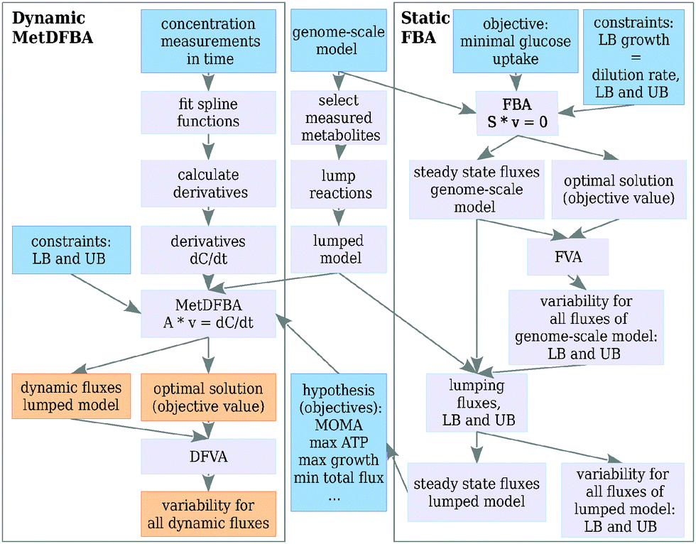

Fig. 1 The MetDFBA framework for estimating dynamic flux profiles. The blue boxes indicate input, orange boxes indicate the result. LB and UB are lower and upper bounds for the fluxes v, FBA = flux balance analysis, S = stoichiometry matrix of the genome scale metabolic network, A = stoichiometry matrix used in MetDFBA (explained in text), dC/dt = vector with time derivatives of the concentrations of the metabolites, (D)FVA = (dynamic) flux variability analysis. The right part of the figure (static FBA) shows how to obtain steady state flux distributions and bounds necessary to calculate the flux before the perturbation, needed to calculate the flux at t = 0 and in certain objective functions (e.g. MOMA = minimization of metabolic adjustment).

In case of estimating dynamic fluxes given an assumed objective, the results are compared with flux estimations based on concentration measurements in time and ¹³C mass isotopomer measurements. In contrast to ¹³C MFA, our method only uses metabolite concentration measurements (and not ¹³C mass isotopomer measurements) to estimate the fluxes.

In case of testing hypotheses, different objective functions are implemented. For each objective function, the resulting fluxes are plotted and compared with external information from the literature to decide which hypotheses can be rejected. The different steps in the mathematical framework are described below and details can be found in ref. 25.

2.1 MetDFBA mathematical framework

2.1.1 Flux balance analysis (FBA). Using an appropriate objective function Z, mass balances and reaction rate constraints, flux balance analysis¹⁷ is applied on a genome scale model to obtain the steady state flux (reaction rate) distribution before the perturbation. Fluxes of reactions supposed not to occur under the given experimental conditions (e.g. because a certain substrate is not in the medium) are set to zero. The fluxes are constrained by upper and lower bounds, which have the same sign for irreversible reactions and different sign for reversible reactions. Solving the optimization problem results in optimal steady state fluxes and an optimal value for the objective function Z_opt.

2.1.2 Flux variability analysis (FVA). Because the optimization problem described above is convex the optimal value Z_opt is the global optimum.²⁶ Nevertheless, the optimal fluxes determined in the FBA solution are not always unique. It is possible that the same optimal value Z_opt is achieved by different flux distributions satisfying the constraints.²⁷ This variability of the fluxes at the optimal solutions can be studied with flux variability analysis (FVA).²⁸ Hereto each flux is minimized and maximized, given mass balances, reaction rate constraints and the objective function equal to its optimum. In this way we obtain lower and upper bounds for each flux.

2.1.3 Calculation of derivatives. To avoid large fluctuations in the derivatives due to noise of the metabolite concentration data (C), we used B-splines smoothing.²⁹ Subsequently, the derivatives (dC/dt) are calculated from the splines at equidistant (10 s) time points within the window of observation of the experiments. In the case of multiple metabolite measurements (e.g. both LC/MS and GC/MS measurements, biological replicates), the average of the derivatives was calculated. The results are gathered in an (m × n)-matrix dC/dt (m metabolites, n time points).

2.1.4 Lumping of reactions. Often, not all metabolites in the genome scale model are measured. Therefore, we need to construct a lumped model from the genome scale model that only includes measured metabolites. We use two types of lumping. Type I is done as follows. If there are two reactions and 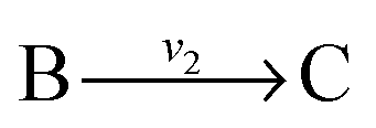, and B is not measured, we lump the reactions by adding them stoichiometrically into 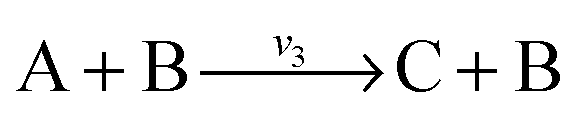. Now B can be omitted resulting in . For type II lumping, two reactions 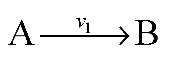and 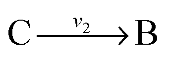with A and C not measured are combined to one arrow, . The steady state flux distribution of the lumped model is calculated from the steady state flux distribution of the genome scale model using the following rules that are valid under steady state. When is lumped to 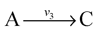, then v₃ = v₁ = v₂. When and with A and C not measured are lumped to 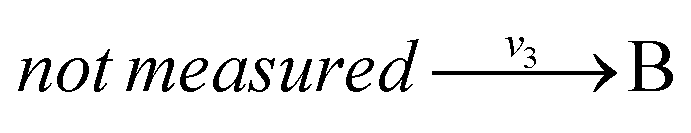, then v₃ = v₁ + v₂. The rule for type I lumping is not valid for the dynamic situation where the time derivatives of the concentrations are not equal to zero. Considering type I lumping, the concentration of B is likely to change temporarily after a perturbation. In this situation fluxes v₂ and v₁ will be unequal. Since B was not measured we cannot estimate v₁ and v₂ but we can estimate v₃ of the lumped reaction. Because we use a least squares method, v₃ will have a value that attempts to estimate the concentration changes of A and C as good as possible in a quadratic sense. So, the magnitude of v₃ is a compromise between v₁ and v₂ and its value will therefore be between the magnitudes of v₂ and v₁. In what follows, we will describe a new method to determine the dynamic behaviour of the fluxes through the lumped reaction scheme.

2.1.5 MetDFBA. MetDFBA is an extension of DFBA.^18,30–32 The dynamic mass balance constraints are of the form dC/dt = S·v. When using both external and internal metabolite balances, it has to be taken into account that the balance space is different (bioreactor and intracellular volume).³³ Therefore, the left-hand side of the mass balances for the external metabolites is multiplied by a factor V_ext/V_int,³⁴ where V_int and V_ext are the intracellular and extracellular volume respectively.

In DFBA, the differential equations are rewritten as linear equations using a finite collocation method.¹⁸ For larger systems DFBA takes an unreasonable amount of computational time. When metabolite concentration measurements are available, the time derivatives dC/dt in the mass balances can be substituted by time derivatives calculated from the data. In this way the differential equation constraints become linear constraints. This makes MetDFBA a computational much simpler problem than DFBA. Consider

where S_l is the stoichiometric matrix of the lumped model and dC/dt are the time derivatives calculated from the measured data. For n time points, r reactions and m metabolites, A is an (n·m × n·r)-matrix and b an (n·m × 1)-vector. A linear optimization problem of the following form is solved:

minimize or maximize F

subject to

A·v_t = b

v_min ≤ v_t ≤ v_max

where F is the objective function after the perturbation; v_t = (v₁(t₁),…,v_r(t_n))^T is the (n·r × 1)-vector of r reactions rates in the lumped model at each of the n time points; v_min and v_max are vectors of lower and upper bounds for the fluxes respectively. An optimum F_opt for the objective function and optimal reaction rate profiles are obtained.

In DFBA with the Dynamic Optimization Approach (DOA),¹⁸ an objective function has the form where t₀ and t_f are the start (steady state) and the end time of the experiment respectively. The integral is approximated with the finite collocation method. In MetDFBA, we write the integral as a sum of integrals over intervals between subsequent time points . We apply the trapezoidal rule on each integral, which means that we approximate the integral (area under the curve) of f(t) by the area of a trapezoid in order to reduce computational complexity.

2.1.6 Dynamic FVA. To study the variability of the optimal fluxes leading to the same optimal value F_opt, a variant of FVA taking into account the non steady state condition is performed. In this variant, the constraints on the fluxes are: A·v_t = b and v_min ≤ v_t ≤ v_max. Furthermore, dynamic FVA is the same as FVA.

3 Results

3.1 Adaptation of Penicillium chrysogenum during feast-famine cycles

The physiology, growth and product formation of a cellular system is the result of a complex interaction between the extracellular environment and the cellular metabolic and regulatory mechanisms. The production capacity of an organism thus strongly depends on the environmental conditions which might be a reason for unexpected scale-up behaviour observed in large-scale fermentation processes and which can lead to reduced biomass yield and reduced product formation.^3,35–39 Estimations of fluxes from intermittent glucose feeding cycles during Penicillium chrysogenum cultivation may lead to new hypotheses on the regulation of metabolism to cope with dynamic environmental conditions and lead to the development of metabolic engineering strategies to improve the product yield.

We compared our estimated fluxes from MetDFBA to fluxes based on isotopomer measurements from de Jonge et al.³ to validate our method, using an assumed objective: the minimization of the sum of squared fluxes. We believe that minimizing the cells total enzyme usage is a reasonable objective during constantly changing environmental conditions (e.g. intermittent feeding). We focused on the upper glycolysis, the pentose phosphate pathway (PPP) and storage metabolism. See Tables S1 and S2 (ESI†) for an overview of the metabolic network and used abbreviations. Intracellular and extracellular metabolite concentrations were measured over time during one feast-famine cycle. Time-series of 17 metabolites, participating in 22 reactions were used to apply our method. The dataset is described in more detail in the ESI,† Section S1. Since xylitol 5-phosphate was not measured we lumped four reactions. We constrained the optimization problem by assuming that most reactions are irreversible (Table S2, ESI†). The feed rate was set experimentally. We aim to test whether MetDFBA, with only concentration measurements in time as input, is capable of estimating dynamic fluxes.

3.1.1 Estimating dynamic flux profiles. The green lines in Fig. 2 show the estimated dynamic fluxes through the upper glycolysis during one feast-famine cycle. Most estimated fluxes through the upper glycolysis approximated the profiles obtained by ¹³C MFA³ (black line Fig. 2) except for the second reaction, the conversion of glucose-6-phosphate (G6P) into fructose-6-phosphate (F6P). Although the shapes of the MetDFBA and ¹³C MFA profiles were similar for this reaction, the MetDFBA flux was significantly lower. This was caused by a too high estimation of flux going into the PPP via the conversion reaction of G6P into 6-phospho-gluconate (P6G, see Fig. S1, ESI†) which was roughly 25 times higher for MetDFBA compared to the ¹³C MFA based flux estimation. Also when considering the distribution of the average fluxes during one feast-famine cycle (See Fig. S3–S6, ESI†) it became obvious that the reduction in flux going through the conversion reaction of G6P into F6P, was caused by the high flux through the oxidative PPP. Because this pathway is more or less circular this flux is going back to the upper glycolysis at nodes F6P and PG3, which explains the better estimations for the fluxes of the upper glycolysis after node F6P. The MetDFBA and ¹³C MFA based fluxes for storage metabolism (See Fig. S2, ESI†) were also comparable except for the conversion reaction of uridine diphosphate glucose (UDP_Glc) into glycogen (Glyc), and the degradation of Glyc into G6P and glucose-1-phosphate (G1P), which had the same order of magnitude but different shapes.

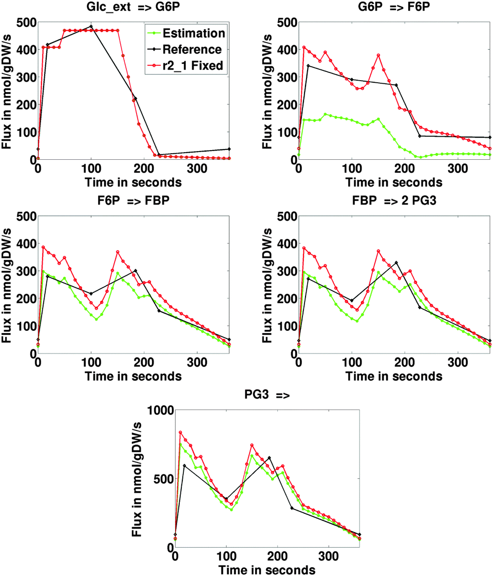Fig. 2 Estimated dynamic fluxes in nmol gDW⁻¹ s⁻¹ through the upper glycolysis in Penicillium. Black indicates the experimental reference (¹³C MFA), green indicates MetDFA estimations, red indicates the MetDFBA fixing the conversion of G6P into 6PG (reaction r2_1).

3.1.2 Using prior knowledge to improve flux estimation. MetDFBA overestimated the flux through the PPP. The results showed that the chosen objective has the property to divide the flux too equal, within the solution space, between the PPP and the rest of the glycolysis. If prior knowledge like kinetic parameters are available the distribution of fluxes at split nodes could be forced towards more realistic ratios. This could be done by calculating the flux for one reaction for which kinetic parameters are available and fix this flux by setting upper and lower bounds of this flux according to the calculated values. To illustrate this we added an additional constraint to the conversion reaction of G6P into 6PG (reaction r2_1). The flux through this reaction was constrained by setting the upper and lower flux bounds for the entire feast-famine cycle to the estimation obtained with the ¹³C MFA approach for this reaction. Subsequently, we recalculated the fluxes. As expected, this resulted in a significant decrease of the fluxes of the entire PPP (red bars in Fig. 3 and red lines in Fig. S1, ESI†). The magnitude and shape of the flux profiles of the conversion reaction of 6PG into Rib5P, and the conversion of 3PG and Sed7P into F6P and E4P, now were comparable to results of the ¹³C estimations.³ In addition, the conversion reaction of G6P into F6P, the first reaction of the glycolysis after the G6P-node, where the flux branches towards the PPP, was now in the same order of magnitude (red line in Fig. 2). The remaining reactions of the PPP were lumped and therefore they could not be compared (Fig. S7, ESI†). Fluxes through storage metabolism were unaffected by the additional constraints. The average fluxes during one feast-famine cycle confirm this observation (Fig. S3–S6, ESI†).

Fig. 3 Estimations of the average fluxes through the considered metabolic network in nmol gDW⁻¹ s⁻¹ including upper glycolysis (r1_2:r1_5), pentose phosphate pathway (r2_1:r2_7) and storage metabolism (trehalose, glycogen and mannitol) in Penicillium. See caption Fig. 2 for a description of the legend.

3.2 Response of Saccharomyces cerevisiae to a glucose pulse

To demonstrate how MetDFBA could be used to test hypotheses about optimality principles we applied our method to time-resolved metabolomics data of the central carbon metabolism in S. cerevisiae grown under aerobic conditions. Short-term perturbation-response experiments were carried out by an extracellular glucose pulse.^24,40,41 Extracellular and intracellular metabolite concentration levels were measured over time. The dataset is described in more detail in the ESI,† Section S2.

A steady state flux distribution required for MetDFBA with minimal glucose uptake as objective, was obtained from FBA applied on a genome scale model of S. Cerevisiae.⁴² When glucose is limited it is realistic to suppose that the glucose uptake is minimal, which was used as objective to obtain the optimal steady state flux distribution. The lower bound of the growth rate was set equal to the dilution rate. The lower and upper bounds of the remaining fluxes were taken from the genome scale model. After lumping and removing reactions that did not occur under the given experimental conditions, the model consisted of 33 metabolites and 62 reactions. The reaction scheme and a detailed list of the reactions are given in Fig. S11 and Table S5 (ESI†).

We applied MetDFBA in conjunction with seven objective functions to establish the most likely response of the organism. Results from MetDFBA were evaluated against the following five criteria:

1. The solution space of optimal flux estimates should be significantly reduced (compared to the solution space defined by the capacity constraints);

2. The directionality of the metabolic reactions should be in agreement with literature;⁴³

3. After a glucose pulse, S. cerevisiae switches from respiratory to respiro-fermentative conditions.⁴⁴ The activity of the TCA cycle, crucial for ATP production under respiratory conditions, becomes low when switching to fermentation;⁴⁵

4. The fluxes for the upper glycolysis (G6P → F6P → FBP → GAP + DHAP) are lower than for the lower glycolysis (GAP → 3PG → PEP → PYR);⁴⁵

5. The qualitative behavior of the fluxes corresponds with the kinetic model simulations of Vaseghi et al. of the pentose phosphate pathway (PPP) in which the reactions rates show a fast increase immediately after the pulse, followed by a very slow decrease.⁴⁶

Objective functions are rejected if the flux profiles do not fit cell physiology.

3.2.1 Optimizing a single objective function. We compared seven objective functions (Table S7, ESI†) on their ability to give biologically meaningful estimates of the flux profiles. These seven functions have the following objectives: maximize biomass production, maximize ATP production, maximize the ATP production in the cytosol, maximize the glucose uptake, maximize the ethanol production, minimize the sum of absolute fluxes and minimize the squared difference of the reaction rates with steady state (MOMA). Each of the seven objective functions is further explained in the ESI,† Section S2.1.

Table S8 (ESI†) shows the results of the evaluation of the five conditions for each of the seven optimization problems shown in Table S7 (ESI†). None of the objectives satisfied all the five criteria mentioned in the previous section.

3.2.2 Multi-objective optimization. It has been proposed that flux changes after a perturbation occur as a result of a combination of maximal metabolic or energetic efficiency under the given conditions, and minimization of adjustment^47,48 or minimization of the sum of absolute fluxes.⁴⁹

Previous studies showed that objective functions compete against each other.^27,47,50 This means that one objective function can only be improved if another is worsened. Optimal solutions for competing objectives are called Pareto optimal.⁴⁷ The set of Pareto optimal solutions is called the Pareto front.⁵¹ A method to calculate Pareto optima is optimizing a weighted sum of the objectives.⁵² The following multi-objective optimization problem is solved:

minimize F = F₁ − w·F₂

subject to

A·v_t = b

v_min ≤ v_t ≤ v_max

where F₁ is MOMA or the sum of absolute fluxes and F₂ is one of the other objective functions of Table S7 (ESI†). An overview of the multi-objective optimization problems solved in this study is given in Table S9 (ESI†). Each value of w determines a point on the Pareto front⁵¹ (Fig. S12, ESI†). In this study, the results of the optimization are shown for w = 10^p (p = −3,…,6).

In Table S10 (ESI†), the results of checking the five criteria for the solutions of the multi-objective optimization problems (Table S9, ESI†) are shown. The MetDFBA fluxes satisfy all five criteria if MOMA is combined with maximization of ethanol production, and if the weight (w) is in the range of 10⁴–10⁶ (the orders of F1, F2 and w·F2 are 10⁷, 10⁵ and 10⁹–10¹¹ respectively; See Fig. 4 and Fig. S13–S15, ESI†). For weights lower than 10⁴, the solution is in contradiction with criterion 5. This implies that maximizing ethanol production (F2) is more important than MOMA (F1). However, only maximizing ethanol did not lead to results satisfying the five evaluation criteria (see Table S7, ESI†). There is no significant difference among the optimal solutions for w = 10⁴, 10⁵ and 10⁶. However, the solution space becomes larger when increasing w.

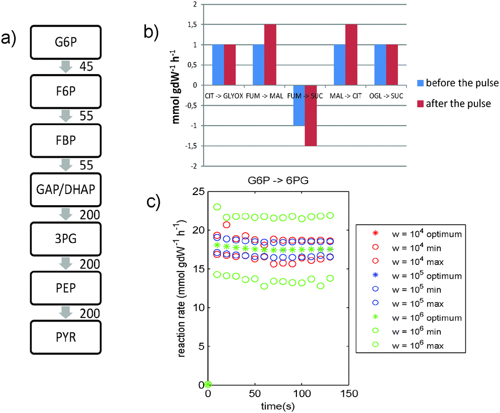Fig. 4 S. cerevisiae study. Results of combining maximize ethanol yield with MOMA. (a) Average fluxes through glycolysis (in mmol gDW⁻¹ h⁻¹) during the first two minutes after the glucose pulse. The flux through lower glycolysis is higher than the flux through upper glycolysis. (b) The fluxes through the TCA cycle remain low compared with the fluxes through the rest of the network (figures a and c). (c) The flux from G6P → 6PG shows a large increase after the pulse, followed by a slow decrease. Similar profiles for the other PPP fluxes are shown in Fig. S16 (ESI†). Legend: optimum = optimal solution found by MetDFBA for the given weight; min and max are lower and upper bounds found by dynamic FVA for the given weight.

4 Implementation details

Optimization problems were solved using the CPLEX⁵³ for MATLAB Toolbox. Smoothing was performed using the splinefit code⁵⁴ for MATLAB.⁵⁵ Pictures of average fluxes through the metabolic network were made with the FluxViz⁵⁶ plugin for Cytoscape.⁵⁷

5 Discussion

We presented MetDFBA, a mathematical framework that directly incorporates time-resolved metabolomics data to perform dynamic flux balance analysis. In comparison to the DFBA method developed by Mahadevan,¹⁸ we could significantly reduce both the number of parameters to estimate and the mathematical complexity. We validated the method by comparing MetDFBA flux estimations to a previous study using ¹³C labeling to identify intracellular fluxes.

In the Penicillium study, it was observed, that a series of intracellular fluxes was estimated comparable to the more complex ¹³C tracer method, except those of the pentose phosphate pathway (PPP). The flux through the PPP was overestimated significantly. This overestimation indicated a property of the applied objective function: the minimal total enzyme usage is obtained by equally distributing the flux at split nodes. Therefore we decided to constrain the entrance reaction of the PPP according to the values obtained in the reference study which indeed improved the results. The choice to fix this flux in particular, was based on the comparison between results and experimental reference, which of course could not be used in situations where this method is applied to predict unknown fluxes. However the split ratios could be further constraint by expert knowledge like kinetic parameters from the literature to calculate particular fluxes. The fluxes should be selected based on the network topology, especially highly connected nodes will require additional constraints.

Additionally we demonstrated how the MetDFBA framework could be used to elucidate the biological objective of a yeast cell through the comparison of different objective functions that represent phenotypes.

For Saccharomyces cerevisiae we showed that minimization of the overall flux and MOMA resulted in a significantly reduced solution space for the fluxes, as determined by dynamic FVA. These results can be explained by the fact that both these objectives constrain all fluxes while the other objectives only constrain flux(es) corresponding to a specific metabolite. The MOMA solution for glycolysis and the TCA cycle was in accordance with the physiological information in the literature, but the qualitative behaviour of the estimated fluxes for the pentose phosphate pathway did not correspond to the model simulations of Vaseghi.⁴⁶ However, when combining MOMA with maximization of the ethanol yield, the five evaluation criteria (see Section 3.2.) were fulfilled. These results show that maximizing ethanol yield is very important compared to MOMA, but only maximizing ethanol did not lead to results satisfying all five evaluation criteria (see Table S7, ESI†). The results of this case study show that optimizing the yield or uptake of a single compound was insufficient to significantly reduce the solution space of reaction rate profiles determined by the capacity constraints. A reduced solution space could only be obtained from at least two objectives or from one objective that is a function of all the fluxes. From this case study it can be concluded that both the objectives MOMA and ethanol production are important. In biological terms this means that yeast converts the glucose to ethanol with as little as possible adaptations to the steady state fluxes.

MetDFBA requires the measurement of (all) extracellular and intracellular metabolite concentrations in response to perturbations. Because of the low intracellular amounts and high flux, methods for rapid sampling and quenching are required. With current, quantitative metabolomics approaches using MS technologies about 100–150 metabolites, especially of central carbon metabolism can be obtained. Computationally, MetDFBA is a linear programming problem with can easily scale to genome scale models. For dynamic ¹³C flux identification, the microorganism is supplied with labeled substrate. Next to the metabolite concentrations, the labeling enrichment of the metabolites is measured. This results in the double amount of samples and mass isotopomer measurements. Generally, if the concentration can be measured, also the mass isotopomer enrichments can be measured. Computationally, flux identification using ¹³C metabolic flux analysis requires to balance metabolites as well as labeling states. In contrast to metabolite balances, the labeling balances lead to non-linear differential equation systems that require advanced computation, even at metabolic steady-state.^58,59 The parameter identification, and especially obtaining the global optimum are challenging already for medium sized networks (order of 100 metabolites). In general dynamic ¹³C metabolic flux analysis is experimentally and computationally more intensive than MetDFBA.

We presented the incorporation of time-resolved metabolomics data into DFBA. Considering the upcoming availability of high-throughput expression data of the last decade, it is probably a logical next step to further develop MetDFBA to make it also suitable for the integration of expression data. Several methods that combined expression data with FBA were recently published.^60–62 They all have in common that they try to further reduce the flux distribution solution space. Some use an arbitrary threshold above which corresponding reactions are assumed to be inactive and excluded. For MetDFBA the ones that constrain the maximum possible flux through the reaction, according to the expression levels of the corresponding enzymes, are probably most suitable because MetDFBA uses a predefined network. More tight constraints will probably result in more accurate solutions and with a smaller solution space, a smaller (more lumped) network might be satisfactory and thus fewer metabolite measurements might be needed. Another potentially interesting approach to further reduce the solution space is the addition of extra energy balance constraints, as described by Beard et al.,⁶³ which ensures that all estimated fluxes are thermodynamically feasible. Finally, when available, kinetic descriptions about metabolic regulation (e.g. allosteric activation or inhibition) can be easily incorporated into the constraints in a similar way as described by Chowdhury et al.⁶⁴ for classical FBA.

6 Conclusion

Studying dynamic fluxes and optimization principles is important to understand cellular functioning and adaptation to changing environments. In this study, we proposed a new method, MetDFBA, that combines DFBA with time-resolved metabolomics experiments to overcome the limitations of classical DFBA. In this paper, we discussed two applications of MetDFBA. When it is known which objective drives an organism under certain perturbations, MetDFBA can be used to estimate dynamic flux profiles. A second application of MetDFBA is testing hypotheses about objectives driving cellular behaviour under perturbations. MetDFBA does not require detailed kinetics but, when available, kinetic information can be easily incorporated in the constraints. MetDFBA can include multiple objective functions by using a weighted sum of the objective functions. Method validation with ¹³C mass isotopomer measurements confirmed that MetDFBA can accurately estimate dynamic flux profiles using a minimal amount of kinetic information, given the objective driving the organism under the conditions in the experiment. Evaluation with prior information from the literature confirmed that MetDFBA is also suitable for testing hypotheses about objectives driving cellular behaviour under changing environments.

Author contributions

AMW and DMH contributed equally to this manuscript and share first authorship. AMW performed MetDFBA on the Penicillium chrysogenum case study. DMH developed the MetDFBA together with HCJH, and performed the S. cerevisiae case study. HCJH contributed to the development of the MetDFBA and both case studies. MMWBH provided support to the development of MetDFBA and the S. cerevisiae case study. SAW provided the Penicillium chrysogenum metabolite data. BT provided support to the S. cerevisiae case study. AKS provided support to the development of MetDFBA and the S. cerevisiae case study. AHCvK contributed to the MetDFBA analysis of Penicillium chrysogenum. AMW, DMH, HCJH, AHCvK and AKS drafted the manuscript.

Acknowledgements

This project was financed by the Netherlands Metabolomics Centre (NMC) and the Netherlands Consoritum for Systems Biology (NCSB), which are part of the Netherlands Genomics Initiative – Netherlands Organisation for Scientific Research. The authors are grateful to Gertien Smits (University of Amsterdam) and Frank Bruggeman (Free University of Amsterdam) for giving suggestions for objective functions. We thank André Canelas (TU Delft and Free University of Amsterdam) for providing us with the S. cerevisiae data, Timo Maarleveld (Free University of Amsterdam) for providing us with weblinks to fast software for optimization and for his input in the flux balance analysis, and Perry Moerland (Academic Medical Center, University of Amsterdam) for several valuable discussions about this research.

Notes and references

1. H. Kitano, Nat. Rev. Genet., 2004, 5, 826–837.
2. J. Stelling, Curr. Opin. Microbiol., 2004, 7, 513–518.
3. L. de Jonge, N. Buijs, J. J. Heijnen, W. M. van Gulik, A. Abate and S. A. Wahl, Biotechnol. J., 2014, 9, 372–385.
4. H. Gardener, C. B. Wright, D. Cabral, N. Scarmeas, Y. Gu, K. Cheung, M. S. V. Elkind, R. L. Sacco and T. Rundek, Atherosclerosis, 2014, 234, 303–310.
5. R. Herwig and H. Lehrach, Dialogues Clin. Neurosci., 2006, 8, 283–293.
6. G. Balazsi, A. van Oudenaarden and J. J. Collins, Cell, 2011, 144, 910–925.
7. I. Golding, Annu. Rev. Biophys., 2011, 40, 63–80.
8. A. Kuchina, L. Espinar, J. Garcia-Ojalvo and G. M. Süel, PLoS Comput. Biol., 2011, 7, e1002273.
9. T. J. Perkins and P. S. Swain, Mol. Syst. Biol., 2009, 5, 326.
10. A. Paldi, Prog. Biophys. Mol. Biol., 2012, 110, 41–43.
11. J. Nielsen, J. Bacteriol., 2003, 185, 7031–7035.
12. Y. Matsuoka and K. Shimizu, Biochem. Eng. J., 2010, 49, 326–336.
13. B. Teusink, J. Passarge, C. A. Reijenga, E. Esgalhado, C. C. van der Weijden, M. Schepper, M. C. Walsh, B. M. Bakker, K. van Dam, H. V. Westerhoff and J. L. Snoep, Eur. J. Biochem., 2000, 267, 5313–5329.
14. W. A. van Winden, J. C. van Dam, C. Ras, R. J. Kleijn, J. L. Vinke, W. M. van Gulik and J. J. Heijnen, FEMS Yeast Res., 2005, 5, 559–568.
15. J. O'Grady, J. Schwender, Y. Shachar-Hill and J. A. Morgan, J. Exp. Bot., 2012, 63, 2293–2308.
16. W. Wiechert, Metab. Eng., 2001, 3, 195–206.
17. J. D. Orth, I. Thiele and B. O. Palsson, Nat. Biotechnol., 2010, 28, 245–248.
18. R. Mahadevan, J. S. Edwards and F. J. Doyle, Biophys. J., 2002, 83, 1331–1340.
19. R. S. Costa, D. Machado, I. Rocha and E. C. Ferreira, IET Syst. Biol., 2011, 5, 157–163.
20. S. B. Crown, W. S. Ahn and M. R. Antoniewicz, BMC Syst. Biol., 2012, 6, 43.
21. J. Forster, I. Famili, P. Fu, B. O. Palsson and J. Nielsen, Genome Res., 2003, 13, 244–253.
22. A. Varma and B. O. Palsson, Nat. Biotechnol., 1994, 12, 994–998.
23. R. Schuetz, L. Kuepfer and U. Sauer, Mol. Syst. Biol., 2007, 3, 119.
24. A. B. Canelas, W. M. van Gulik and J. J. Heijnen, Biotechnol. Bioeng., 2008, 100, 734–743.
25. D. M. Hendrickx, PhD thesis, University of Amsterdam, the Netherlands, 2013.
26. D. G. Luenberger, Introduction to linear and nonlinear programming, Addison-Wesley, 1973.
27. C. E. García Sánchez and R. G. Torres Sáez, Biotechnol. Prog., 2014, 30, 985–991.
28. R. Mahadevan and C. H. Schilling, Metab. Eng., 2003, 5, 264–276.
29. T. Hastie, R. Tibshirami and J. Friedman, The elements of statistical learning. Data mining, inference and prediction, Springer-Verlag, New York, 2001.
30. J. M. Lee, E. P. Gianchandani and J. A. Papin, Briefings Bioinf., 2006, 7, 140–150.
31. R. Y. Luo, S. Liao, G. Y. Tao, Y. Y. Li, S. Zeng, Y. X. Li and Q. Luo, Mol. Syst. Biol., 2006, 2, 2006.0031.
32. S. Kleessen and Z. Nikoloski, BMC Syst. Biol., 2012, 6, 16.
33. A. B. Canelas, A. ten Pierick, C. Ras, R. M. Seifar, J. C. van Dam, W. M. van Gulik and J. J. Heijnen, Anal. Chem., 2009, 81, 7379–7389.
34. I. C. Chou and E. O. Voit, BMC Syst. Biol., 2012, 6, 84.
35. L. P. de Jonge, N. A. A. Buijs, A. ten Pierick, A. Deshmukh, Z. Zhao, J. A. K. W. Kiel, J. J. Heijnen and W. M. van Gulik, Biotechnol. J., 2011, 6, 944–958.
36. A. Lapin, M. Klann and M. Reuss, Adv. Biochem. Eng./Biotechnol., 2010, 121, 23–43.
37. N. M. Oosterhuis and N. W. Kossen, Biotechnol. Bioeng., 1984, 26, 546–550.
38. A. R. Lara, E. Galindo, O. T. Ramrez and L. A. Palomares, Mol. Biotechnol., 2006, 34, 355–381.
39. G. Larsson, M. Tornkvist, E. S. Wernersson, C. Tragardh, H. Noorman and S. O. Enfors, Bioprocess Eng., 1996, 14, 281–289.
40. D. M. Hendrickx, H. C. J. Hoefsloot, M. M. W. B. Hendriks, A. B. Canelas and A. K. Smilde, Anal. Chim. Acta, 2012, 719, 8–15.
41. T. Kamminga, MSc thesis, Department of Biotechnology, Delft University of Technology, 2007.
42. B. D. Heavner, K. Smallbone, B. Barker, P. Mendes and L. P. Walker, BMC Syst. Biol., 2012, 6, 55.
43. A. B. Canelas, C. Ras, A. ten Pierick, W. van Gulik and J. J. Heijnen, Metab. Eng., 2011, 13, 294–306.
44. M. T. A. P. Kresnowati, W. A. van Winden, M. J. H. Almering, A. ten Pierick, C. Ras, T. A. Knijnenburg, P. Daran-Lapujade, J. T. Pronk, J. J. Heijnen and J. M. Daran, Mol. Syst. Biol., 2006, 2, 49.
45. O. Frick and C. Wittmann, Microb. Cell Fact., 2005, 4, 3.
46. S. Vaseghi, A. Baumeister, M. Rizzi and M. Reuss, Metab. Eng., 1999, 1, 128–140.
47. R. Schuetz, N. Zamboni, M. Zampieri, M. Heinemann and U. Sauer, Science, 2012, 336, 601–604.
48. D. Molenaar, R. van Berlo, D. de Ridder and B. Teusink, Mol. Syst. Biol., 2009, 5, 323.
49. E. S. Snitkin and D. Segré, Genome Inf., 2008, 20, 123–134.
50. D. Nagrath, M. Avila-Elchiver, F. Berthiaume, A. W. Tilles, A. Messac and M. L. Yarmush, Ann. Biomed. Eng., 2007, 35, 863–885.
51. S. J. Kim and D. J. Volsky, BMC Bioinf., 2005, 6, 144.
52. T. D. Vo, H. J. Greenberg and B. O. Palsson, J. Biol. Chem., 2004, 279, 39532–39540.
53. IBM® ILOG CPLEX® Optimization Studio, V12.2, Microsoft Windows XP Version 5.1., Copyright©, 1987-2010, IBM Corp.
54. J. Lundgren, Splinefit, http://www.mathworks.com/matlabcentral/fileexchange/13812-splinefit, retrieved September 26, 2011.
55. MATLAB, Version 7.11.0, Copyright©, 1984–2010, The Mathworks Inc.
56. M. König and H.-G. Holzhütter, Genome informatics. International Conference on Genome Informatics, 2010, 24, 96–103.
57. M. E. Smoot, K. Ono, J. Ruscheinski, P.-L. Wang and T. Ideker, Bioinformatics, 2011, 27, 431–432.
58. M. Weitzel, K. Nöh, T. Dalman, S. Niedenführ, B. Stute and W. Wiechert, Bioinformatics, 2013, 29, 143–145.
59. K. Nöh, A. Wahl and W. Wiechert, Metab. Eng., 2006, 8, 554–577.
60. A. Navid and E. Almaas, BMC Syst. Biol., 2012, 6, 150.
61. E. Resnik, P. Metha and D. Segré, PLoS Comput. Biol., 2013, 9, e1003195.
62. A. S. Blazier and J. A. Papin, Front. Physiol., 2012, 3, 299.
63. D. A. Beard, S.-d. Liang and H. Qian, Biophys. J., 2002, 83, 79–86.
64. A. Chowdhury, A. R. Zomorrodi and C. D. Maranas, PLoS Comput. Biol., 2014, 10, e1003487.

---

Footnotes

† Electronic supplementary information (ESI) available. See DOI: 10.1039/c4mb00510d

‡ These authors contributed equally to this work.

---