Electronic excitations in molecular solids: bridging theory and experiment

Abstract

As the spatial and temporal resolution accessible to experiment and theory converge, computational chemistry is an increasingly powerful tool for modelling and interpreting spectroscopic data. However, the study of molecular processes, in particular those related to electronic excitations (e.g. photochemistry), frequently pushes quantum-chemical techniques to their limit. The disparity in the level of theory accessible to periodic and molecular calculations presents a significant challenge when modelling molecular crystals, since accurate calculations require a high level of theory to describe the molecular species, but must also take into account the influence of the crystalline environment on their properties. In this article, we briefly review the different classes of quantum-chemical techniques, and present an overview of methods that account for environmental influences with varying levels of approximation. Using a combination of solid-state and molecular calculations, we quantitatively evaluate the performance of implicit-solvent models for the [Ni(Et₄dien)(η²-O,ON)(η¹-NO₂)] linkage-isomer system as a test case. We focus particularly on the accurate reproduction of the energetics of the isomerisation, and on predicting spectroscopic properties to compare with experimental results. This work illustrates how the synergy between periodic and molecular calculations can be exploited for the study of molecular crystals, and forms a basis for the investigation of more challenging phenomena, such as excited-state dynamics, and for further methodological developments.

---

1 Introduction

Continuous improvements in spectroscopic techniques, such as the advent of next-generation X-ray free-electron laser (XFEL) facilities, are allowing the structural dynamics of molecular crystals to be studied in unprecedented detail. These advances bring with them, however, a number of significant challenges in interpreting the data in terms of processes occurring at the molecular level. The length and timescales accessible to these advanced experimental techniques are rapidly converging on those which are accessible to theoretical study, and as such computational chemistry, e.g. within the ubiquitous density-functional theory (DFT) framework, can be a powerful complement to experiment.

A particular problem arises with the study of molecular solids, namely that the calculations need to capture both the chemistry of the molecular species, and the influence of the crystalline environment. At present, there exists a large disparity between the level of theory which is accessible to molecular and solid-state (periodic) calculations, due to the higher complexity of the latter. However, accurate descriptions of molecular properties, particularly those related to electronic excitations, e.g. absorption spectra and excited-state dynamics, frequently require high-level methods. Through continual advances in computing power and software efficiency, the gap between molecular and solid-state calculations is closing, but at present molecular crystals still frequently stretch the limits of what is possible in periodic calculations, mainly due to their large unit cells, and to the spectrum of weak non-bonding interactions which play an important role in defining their structure and properties.

To study electronic excitations in molecular solids, therefore, approximate methods of accounting for the effect of the crystalline environment in molecular calculations are required. In this work, we review several different approaches, and evaluate quantitatively the performance of the simplest one for computing various properties of the well-studied [Ni(Et₄dien)(η²-O,ON)(η¹-NO₂)] linkage-isomerisation system. The key focus of our work is to explore how best to exploit the synergy between solid-state and molecular calculations, and to provide new theoretical insight to complement ongoing experimental work on this and related systems.

Towards chemical accuracy: the “Jacob's ladder” of approximations

Quantum chemistry aims to model the properties of quantum-mechanical systems from first principles by solving the Schrödinger equation, typically within the Born–Oppenheimer (clamped-nuclei) approximation. The ultimate goal is to be able to predict properties with “chemical accuracy”, that is, accuracy on the same scale as state-of-the-art experimental techniques. For example, historically, chemically-accurate energies are usually taken as implying an uncertainty of less than 1 kcal mol⁻¹ (4.18 kJ mol⁻¹), although tighter criterion are often required in practice. Due to Perdew and coworkers,¹ quantum chemistry techniques can be classified according to a “Jacob's ladder” of approximations, extending to the “heaven” of chemical accuracy.

DFT, which recasts the many-body Hamiltonian in the electronic Schrödinger equation into a functional of the spatial electron density n(r),^2,3 is perhaps the most widely-used theoretical “workhorse” at present. Leaving aside implementation details, such as the mathematical basis used to express the electron orbitals, the key parameter in DFT is the form of the exchange–correlation (XC) functional used to calculate the contributions to the total energy from quantum-mechanical electron exchange and correlation. The simplest functional form is the local-density approximation (LDA), in which the exchange and correlation energy for a given n(r) are obtained using a homogenous electron gas as a model system. For some systems, the LDA benefits from a fortuitous cancellation of errors and performs far better than expected, but, in general, it is too big an approximation to model subtle properties accurately.

The LDA can be improved upon substantially by also including the gradient of the electron density, ∇n(r), which forms the basis for semi-local generalised-gradient approximation (GGA) functionals. The logical extension to these are the meta-GGA functionals, which include the second derivative of the electron density, usually in the form of the electron kinetic-energy density τ(r). At the next level, more accurate functionals can be obtained by replacing a fraction of the DFT exchange energy with the exact Hartree–Fock exchange, and such “hybrid” functionals then require the electron orbitals, as well as n(r), as input. Hybrid functionals are standard in molecular quantum-chemistry, and are used routinely for accurate electronic-structure calculations on periodic systems.

Finally, there exist a growing number of “beyond DFT” and “post Hartree–Fock” methods, which are becoming increasingly popular and accessible with advances in computing power. Examples of this include GW theory,⁴ a perturbative approach to treating many-body physics, and second-order Møller–Plesset perturbation theory⁵ (MP2) and coupled-cluster theory,⁶ which both aim at a more accurate description of electron correlation.

In practice, (meta-)GGA functionals typically offer a good balance between computational cost and accuracy for a number of properties, including energetics and forces, and hence equilibrium geometries and vibrational frequencies.⁷ Hybrids usually give more accurate electronic structures (i.e. orbital energies in molecular systems) than semi-local functionals, and so are often a prerequisite for the computation of optical properties and for studying electronic excitations in time-dependent DFT (TD-DFT) calculations. Post-DFT methods are useful in cases where even higher accuracy is required, e.g. to construct benchmark datasets against which functionals can be tested, and are sometimes necessary for systems where many-body effects are prominent, for which the more approximate approaches frequently fail.

Environmental effects in molecular calculations: a spectrum of approaches

The most common methods for accounting for the solid-state environment in calculations on the component species in molecular crystals may be divided into three classes, with differing computational cost and accuracy.

At one end of the scale, full periodic calculations can be performed. The molecular environment is treated explicitly, but the computational cost of using high-level theories is prohibitive for large systems, and lower-level theories may be insufficient to describe certain properties with the required level of accuracy. At the other end, continuum models⁸ (e.g. the polarisable-continuum model (PCM)⁸ or COnductor-like Screening MOdel (COSMO)⁹ schemes) assume that the most important environmental effects can be captured by a simple dielectric screening. This is likely to be a good approximation when the intermolecular interactions are minimal, and is commonly used to implicitly model the effect of a solvent. Forming a “middle ground” between these techniques are embedding methods, in which a large system is separated spatially into different regions which are then treated at different levels of theory.

Explicit periodic calculations

With current hardware and software algorithms, it is feasible to perform periodic calculations on medium-sized molecular crystals (up to a few hundred atoms) using DFT with semi-local (meta-)GGA functionals, or, in some cases, with hybrids.^10–13 This is usually sufficient for studying equilibrium geometry and lattice dynamics (e.g. vibrational frequencies), but semi-local functionals are often not able to describe electronic structure quantitatively, as is required, for example, for accurate prediction of optical properties.

A particular issue with molecular crystals, as opposed to many simple bulk materials, is that weak interactions (e.g. van der Waals' dispersion forces) often play an important role in defining the structure.^14–16 Dispersion forces are, in principle, a non-local electron-correlation effect, and thus a first-principles quantum-chemical description requires a non-local functional. To circumvent this, several approximate methods have been developed to correct GGA energies and forces, e.g. the DFT-D2 ¹⁷/D3 ¹⁸ and DFT-TS¹⁹/TS + SCS²⁰ methods, and non-local correlation functionals such as vdW-DF²¹/DF2.²² However, these approximate forms may not account for more complex many-body dispersion interactions, which appear to be significant in some molecular systems.¹⁶

A good compromise to obtain accurate electronic properties is to optimise structures at a moderate level of theory, and to then perform more accurate single-shot calculations with hybrid functionals. In many cases, this approach gives good results, but for systems where many-body effects are prominent, e.g. excitonic effects in optical spectra,²³ the required higher levels of theory sometimes cannot be used due to computational limitations. Also, since geometry relaxation with non-local functionals is not feasible, it is not realistically possible to study excited-state dynamics with periodic calculations, which precludes the investigation of photochemical reactions.

Embedding

In typical embedding methods, a large bulk system is divided into regions, and the core (e.g. a single molecule, or a dimer, etc.) is treated with a quantum-mechanical (QM) method, while a surrounding “shell” is treated with an empirical molecular-mechanics (MM) method such as a parameterised force field, reverting to a continuum model at larger distances. The layers are then interfaced together to account for the interaction energy between them. The MM atoms are treated as point charges or multipoles, which can polarise the wavefunction in the QM region, while the QM atoms can likewise exert forces on the MM atoms. This allows for an explicit atomistic treatment of large systems, with high accuracy in a region of interest, at a manageable computational cost. This QM/MM approach is commonly used to model biochemical systems, for example to look at redox processes at the active centres of enzymes.

The idea behind QM/MM embedding schemes can be extended to analogous QM/QM methods, where the core region is treated with a high-level quantum-chemical method (e.g. MP2 or coupled-cluster) and the shell with a lower-level one such as DFT with a GGA functional.^24–27 This class of methods also encompasses techniques in which the periodic wavefunctions obtained from an extended-system calculation are converted to localised orbitals, and selected local states then treated with higher-level theories.^28,29

Embedding schemes have successfully been applied to a variety of molecular crystals,^30–32 and the particularly ambitious study by Kochman et al.³² utilised a scheme where a single molecule in a periodic DFT calculation was treated with a molecular code, allowing exploration of its excited-state potential energy surface using TD-DFT.

Continuum models

At the lowest level of approximation, environmental effects can be included using continuum models, which assume that the main influence of surrounding molecules is a dielectric-screening effect. The key parameter in these models is the static dielectric constant of the medium, ε_static, which captures its ability to screen an applied electric field. These methods are routinely used to model solvent effects in molecular calculations, but could also feasibly be used for molecular crystals, provided that the interaction between molecular units is negligible.

The molecule is treated as being a solute within a cavity, surrounded by a dielectric continuum of the solvent. The charge–density cloud of the molecule polarises the medium, which responds by generating screening charges on the cavity surface. In the COSMO model, the screening charges are obtained by modelling the response of an ideal solvent with ε_static = ∞, which is then scaled to account for the ε_static of a non-ideal medium. Some continuum models additionally contain the shape of the solvent molecule as a parameter, which is then taken into account when defining the cavity around the solute.

Continuum models are widely used in the study of solution chemistry (e.g. solution thermodynamics³³ and reactions^34,35), and to model biochemical systems.³⁶ They have also been used to model environmental effects on electronic excitations,^37,38e.g. within a PCM/TD-DFT formalism.³⁸ Continuum models are generally used in quantum chemistry to model solvents, although there are a few cases where they have been employed to model the dielectric environment of a crystal in a molecular calculation.^39,40

Test system: linkage isomerisation in [Ni(Et₄dien)(η²-O,ON)(η¹-NO₂)]

Solid-state linkage isomerisation is a topical example of a reversible phase transition generating one or more metastable structural isomers in response to external stimuli, e.g. illumination or temperature changes.⁴¹ Since the initial observation by Coppens et al. of linkage isomerisation in sodium nitroprusside,⁴² several families of linkage-isomer systems have been discovered, among which Ni–NO₂ (ref. 39 and 43–47) and Ru–SO₂ (ref. 48–51) complexes are perhaps the most well-known.

Linkage-isomer systems are typically studied using photocrystallography, where a sample, usually a single crystal, is irradiated in situ on the diffractometer, allowing the steady-state populations of the different isomers to be quantified as a function of temperature and of the wavelength of radiation used.⁵² By performing pseudo-steady-state experiments, where the crystal is continuously irradiated during the data-collection process,⁴¹ additional short-lived metastable species can also be identified.⁴⁶

The [Ni(Et₄dien)(η²-O,ON)(η¹-NO₂)] linkage-isomer system is an ideal test case for continuum models. The isomerisation takes place within a large reaction cavity, which allows the ligand binding to be switched without inducing a large stress on the crystal.^39,40,43,51 Furthermore, previous computational modelling⁴⁰ and experimental measurements of the transition kinetics⁴⁶ both suggest that, to a good approximation, the molecules in the solid behave as isolated units, whose properties and behaviour are influenced by the dielectric environment of the crystal.

This system exists as three isomers, in which the η¹-bound NO₂ ligand coordinates to the Ni centre via either N or O (Fig. 1). The N-bound ground-state (GS) isomer is obtained on cooling the crystal in the absence of illumination, and is the thermodynamically-stable form. The GS can be converted to the O-bound MS1 isomer with excellent yield on photoactivation, and is also formed thermally in significant population at moderate temperatures. A second O-bound isomer, MS2, was recently observed as a transient species close to the so-called metastable limit, the temperature at which MS1 begins to decay thermally, and can interconvert with MS1 with a relatively small energy barrier.⁴⁰

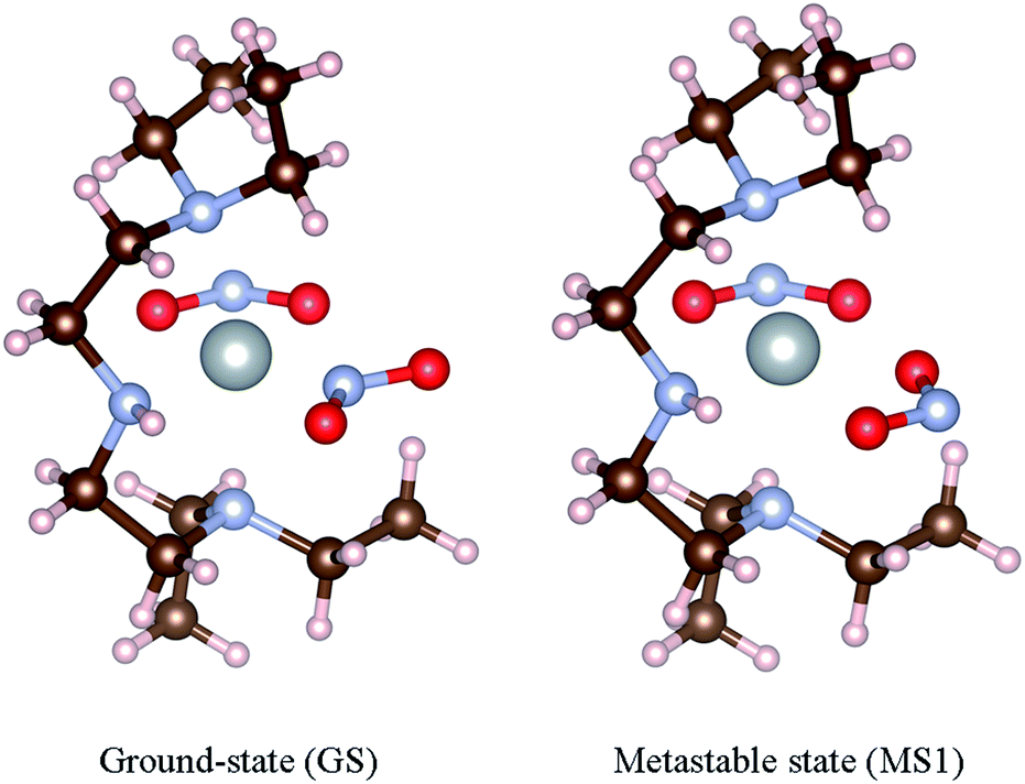Fig. 1 Geometries of the [Ni(Et₄dien)(η²-O,ON)(η¹-NO₂)] isomers. The left-hand image shows the ground-state (GS) N-bound isomer, and the right-hand image shows the metastable O-bound MS1 isomer. These structures were taken from the data in Hatcher et al.⁴⁴

A number of open questions remain on linkage isomerisation. Firstly, although the isomers themselves have been characterised, understanding the reaction paths which connect them is a work in progress.^53–55 Numerical modelling has allowed mechanisms to be proposed for some systems,^39,40 although explicit study of the excited-state potential energy surfaces, and establishing the photochemical-isomerisation pathways, remains an important undertaking. A second key challenge is to understand the role that the crystalline environment plays in controlling the kinetics and energetics of the process, which would, in principle, provide valuable input to crystal-engineering approaches for tuning the properties of different systems for specific applications.

In the present work, we focus on the GS and MS1 isomers, since these have been well characterised experimentally,^44,46 providing a good set of reference data against which to optimise computational parameters and to evaluate the performance of continuum models.

2 Methods

All computational work was performed within the Kohn-Sham DFT formalism.³ Different codes were used for the periodic and molecular calculations, as outlined below.

Periodic calculations

Periodic plane-wave pseudopotential calculations were performed using the Vienna Ab initio Simulation Package (VASP) code.⁵⁶ Projector augmented-wave (PAW) pseudopotentials^57,58 were used to treat core electrons, with the outer s and p electrons of H, N and O, and the 4s, 3d and semicore 3p states of Ni, being treated as valence states. Where available, we used “hard” pseudopotentials, with a smaller core region to allow for more flexibility in the description of the valence wavefunctions. A kinetic-energy cutoff of 944.5 eV was used for the plane-wave basis, and the electronic wavefunctions were evaluated at the Γ point; these parameters were found to be sufficient to converge the total energies to within less than 1 meV per atom. Spin-polarisation was used in all calculations, with each Ni complex constrained to have a triplet magnetic configuration, as was established to be the lowest-energy state in previous work.⁴⁰

A selection of DFT exchange–correlation (XC) functionals were used in these calculations, as described in the text: we tested the PBE⁵⁹ and PBEsol⁶⁰ GGA functionals, the TPSS⁶¹meta-GGA, the dispersion-corrected PBE-D2,¹⁷ PBE-D3 ¹⁸ and TPSS-D2 functionals, and the PBE0 hybrid.⁶²

Convergence criteria of 10⁻⁶ and 10⁻⁵ eV were employed during electronic minimisation and atom position/unit-cell parameter optimisations, respectively. During the calculation of the dielectric functions, as described in the text, the number of electronic bands was increased to 1136, triple the default, to ensure convergence of the sum over empty electronic states. To obtain a high resolution for the calculated function, the number of grid points used to evaluate the electronic density of states (DOS) was increased to 5000 or 10 000, depending on whether or not the resulting function was to be used to compute optical properties.

Molecular calculations

Molecular calculations were carried out using the NWChem⁶³ and Gaussian 09 ⁶⁴ codes. As described in the text, several Pople split-valence⁶⁵ and Dunning⁶⁶ basis sets were tested for the light atoms, together with the Los Alamos effective-core pseudopotential and corresponding double-zeta basis set (LANL2DZ) for the Ni atom.⁶⁷ As in the VASP calculations, the molecular complex was constrained to have a triplet magnetic configuration. For comparison with the periodic calculations, we tested PBE, PBE-D2 and TPSS, and we also used the M06 ⁶⁸ and B3LYP⁶⁹ functionals, which are both popular choices for molecular calculations. Convergence criteria of 10⁻⁶ and 10⁻⁵ were used for the total energy and density, respectively, while geometry optimisations were performed to a force tolerance of 5 × 10⁻⁴ Hartree per Bohr. For the continuum calculations, we tested the COnductor-like Screening MOdel (COSMO) method,⁹ as implemented in NWChem, and the polarisable-continuum model (PCM) in Gaussian.

Vibrational spectroscopy

Room-temperature infrared (IR) and Raman spectra of crystalline [Ni(Et₄dien)(η²-O,ON)(η¹-NO₂)] were collected for comparison with calculated vibrational spectra. IR spectra were obtained from a single crystal using a Perkin Elmer Spectrum 100 FT-IR spectrometer with the ATR accessory. A spectral resolution of 1 cm⁻¹ between 4000 and 600 cm⁻¹ was available with this instrument, and acquisition and processing was performed using the Perkin Elmer Spectrum software.

Raman spectra were collected from a single crystal using a Renishaw inVia Raman spectrometer with the Renishaw WiRE 4.1 software. A 532 nm excitation laser (Renishaw diode laser, 380 mW at source/1.9 mW after attenuation) was used with a 20× objective lens (LEICA), and the instrument was calibrated to the 520 cm⁻¹ line of Si. Spectra were obtained between ∼100 and 4000 cm⁻¹ at a resolution of 1.2 cm⁻¹.

It is worth noting that, since the GS-to-MS1 transition is thermally activated, at ambient temperature, and in particular under laser irradiation at 532 nm during the Raman experiments, the spectra are expected to contain bands due to both the GS and MS1 forms.

3 Results

Energetics

Among the most straightforward property to compute with DFT is (relative) total energy. The per-molecule enthalpy difference between the GS and MS1 crystals has been determined from photocrystallographic measurements of the temperature dependence of the isomer populations,⁴⁴ providing a benchmark against which to quantitatively compare calculated energy differences.

In our recent work,⁴⁰ we found that the energetics were sensitive to the computational parameters employed, in particular the DFT functional used and, for molecular calculations, the choice of basis set. As a foundation for testing continuum models, in this section we systematically investigate these dependencies, and quantify the effect of the crystalline environment on the energy differences between the isomers.

To test the effect of the choice of functional on the predicted energetics, we carried out plane-wave pseudopotential calculations on the reported GS and MS1 crystal structures⁴⁴ with six commonly-used functionals, viz. PBE, PBEsol, PBE + D2, PBE + D3, TPSS and TPSS + D2. For each, the atomic positions and unit-cell parameters were fully relaxed, and the per-molecule GS-MS1 energy differences were then calculated from these optimised models; some structural parameters from the models (e.g. lattice parameters, cell volume and bond lengths) are given in the ESI.† To investigate the effect of the crystalline environment on the energetics, we also carried out an equivalent set of calculations on the individual GS/MS1 complexes in the gas phase. These were performed by placing single molecules from the crystal structures in periodic cells, with an (initial) vacuum gap of 10 Å between images, and optimising the geometries.

Of the selection of functionals we employed, PBE represents a typical choice for many solid-state problems, although PBEsol, a variant of PBE revised to better reproduce the properties of solids, is also used routinely. PBE + D2 and PBE + D3 both add a semi-empirical correction to the PBE energies to account for dispersion forces, and are frequently used for systems where weak interactions are expected to be significant. TPSS is a typical meta-GGA functional, and perhaps the most routinely used functional of this type, and we also tested it in combination with the D2 dispersion correction (TPSS + D2).

Fig. 2 compares the per-molecule energy differences in the crystal and in the gas phase. Compared to the experimental enthalpy difference of 9.69 kJ mol⁻¹, all of the functionals apart from TPSS significantly overestimate the energy difference between the GS and MS1 crystals. The PBE energy difference of 14.57 kJ mol⁻¹ is around 1.5× larger than the experimental one, while PBEsol and the three dispersion-corrected functionals overestimate the difference by a factor of two. On the other hand, the TPSS value of 7.75 kJ mol⁻¹ is in remarkably good agreement, suggesting that the improved accuracy of meta-GGA functionals provides a good description of the energetics of this system.

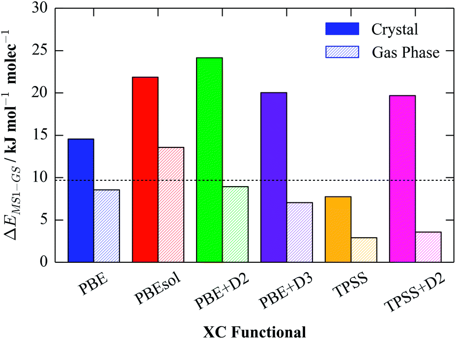Fig. 2 Calculated per-molecule GS-MS1 energy differences in the molecular crystal (solid) and in vacuum (hatched) for a series of different exchange–correlation (XC) functionals. The experimentally-measured enthalpy difference is overlaid as a dashed black line.

Comparing the gas-phase energy differences to those in the solid, all six functionals predict that the difference between the isomers is substantially reduced. However, in all cases it remains positive, indicating that the GS isomer is the ground state in the gas phase as well as in the molecular crystal.

Having found that TPSS gives improved energetics compared to the GGA functionals, we performed single-point energy calculations on our six optimised GS and MS1 structures using the PBE0 hybrid functional, and recalculated the energy differences (see ESI†). We observed some small variation between the different starting geometries, although the calculated values appear to be relatively insensitive to this. The best PBE0 value (7.05 kJ mol⁻¹) is obtained when the atomic positions, but not the cell parameters, are optimised with TPSS as a starting point; it is possible that the agreement might improve further if a geometry optimisation could be performed with the hybrid.

The tight convergence criteria employed in the plane-wave calculations on the molecular species means that the calculated energy differences should be close to the basis-set convergence limit for the molecular calculations. We therefore used these values as a reference to optimise the basis set for these simulations. We carried out single-point energy calculations on the optimised gas-phase GS and MS1 structures with a number of different basis sets, and compared the calculated energy differences to the plane-wave values. Table 1 shows the results for a subset of the basis sets tested and the PBE functional; additional data for PBE, and a corresponding set of data for PBE + D2, are given in the ESI.†

Table 1 Calculated single-molecule GS-MS1 energy differences with the PBE functional and various basis sets. The structures of the complexes are those obtained from the gas-phase plane-wave calculations, and are not re-optimised in these tests

Basis set	ΔEMS1-GS kJ^−1 mol^−1 molec^−1
6-31G	−2.82
6-31G(d)	−3.28
6-31G(d,p)	−3.46
6-311G(d)	3.02
6-311G(d,p)	3.01
6-311+G(d)	5.35
6-311++G(d,p)	4.93
6-311++G(2d,2p)	5.58
cc-pVDZ	−1.47
aug-cc-pVDZ	7.31
cc-pVTZ	7.20
aug-cc-pVTZ	6.51

---

In general, the double-zeta 6-31G family of basis sets predict a qualitatively incorrect energy ordering. Among the triple-zeta basis sets, the accuracy of the predicted energy differences improves when diffuse and polarisation functions are added (6-311G+/++ and 6-311G(d)/(d,p), respectively). This appears to be more important for the heavier atoms, with the 6-311+G(d) basis, which includes diffuse functions and d-type polarisation functions on the heavy atoms, giving very similar results to 6-311++G(2d,2p), which includes diffuse functions and two d/p polarisation functions on both the light and heavy atoms.

We note that the results in Table 1 were all obtained using the LANL2DZ pseudopotential and corresponding double-zeta basis set to treat the Ni atom; during testing, we found that varying the Ni basis made relatively little difference to the energetics when the better-converged basis sets were used for the other atoms (see ESI†), but that, without the pseudopotential, the computational cost was significantly increased.

In contrast to the Pople basis sets, the Dunning bases are designed to give more systematic convergence with respect to the number of basis functions, although they are typically more computationally expensive than the Pople ones. Like the equivalent Pople double-zeta basis sets, the double-zeta cc-pVDZ basis predicts an incorrect energy ordering, while the augmented cc-pVDZ (aug-cc-pVDZ) basis set and the bare and augmented triple-zeta (aug-)cc-pVTZ sets give the best results overall. For the augmented cc-pVDZ and the two cc-pVTZ basis sets, we observed near-quantitative agreement with the plane-wave values for energetics calculations with PBE, PBE + D2 and TPSS (Fig. 3), suggesting that the energy difference with these basis sets is close to the convergence limit.

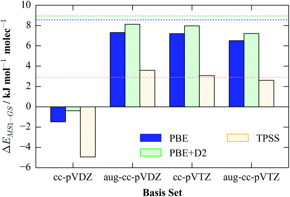Fig. 3 Calculated single-molecule GS-MS1 energy differences with four Dunning basis sets and the PBE, PBE + D2 and TPSS functionals. As for the values in Table 1, the structures of the complexes are those obtained from the corresponding gas-phase plane-wave calculations, and are not re-optimised. For comparison, the reference plane-wave values are overlaid as dashed lines.

We note that these basis sets are computationally expensive to work with, and we found them unwieldy for geometry optimisation; however, the results in Table 1 suggest that a good compromise would be to optimise with the more efficient 6-311+G(d) basis, and to then perform further calculations with one of the triple-zeta Dunning bases where possible, which is the approach taken in the following sections.

Dielectric properties

In this section, we calculate the macroscopic dielectric constants of the molecular crystals from solid-state calculations, and evaluate the performance of the implicit-solvent COSMO model in including the effect of the crystalline environment in the molecular calculations.

As discussed in Section 1, the static dielectric constant (permittivity), ε_static, of a material measures its ability to screen an applied electric field, and as such can be used to model approximately the effect of a dielectric continuum (e.g. a solvent) on various properties of a molecular system. ε_static can be decomposed into the sum of two contributions, viz. electronic polarisation, and ionic relaxation:⁷⁰

ε_static = ε_polarisation + ε_ionic (1)

ε _polarisation can be calculated either from the response of the system to a finite electric field (e.g. using density-functional perturbation theory (DFPT)), or obtained as the zero-frequency component of the real part of the frequency-dependent dielectric function (ε(E) = ε_r(E) + iε_i(E)). Calculating ε_ionic requires additionally the vibrational modes of the system to be evaluated, which for large systems can be very time consuming.

In the current version of the VASP code, ε_polarisation can be computed using DFPT, or by calculating the dielectric function via the linear optical response, while both components of ε_static can be calculated by combining a DFPT calculation of ε_polarisation with a DFPT phonon calculation. However, VASP currently does not support DFPT calculations with semi-empirical and meta-GGA functionals, and thus we were only able to calculate both components of ε_static with PBE and PBEsol. For the other functionals, we obtained the value of ε_polarisation by calculating the dielectric function. Table 2 lists the values of ε_polarisation, ε_ionic and ε_static for the GS and MS1 crystals obtained with PBE and PBEsol, and the corresponding values of ε_polarisation computed with a selection of other functionals are listed in Table 3.

Table 2 Dielectric constants of the GS and MS1 crystal structures, computed with PBE and PBEsol. Each row gives the calculated values of ε_polarisation, ε_ionic, and the sum, ε_static

System	Functional	ε polarisation	ε ionic	ε static
GS	PBE	2.414	1.144	3.558
	PBEsol	2.652	0.971	3.623
MS1	PBE	2.369	0.715	3.084
	PBEsol	2.592	0.714	3.305

---

Table 3 High-frequency dielectric constants (real components of the optical dielectric functions at zero photon energy) (ε_polarisation) of the GS and MS1 crystal structures, computed with a selection of functionals. Calculations with the PBE0 functional were carried out on the fully-optimised PBE, PBEsol and TPSS structures, which is denoted by “PBE0@XC”

Functional	ε polarisation
	GS	MS1
TPSS	2.582	2.535
PBE-D2	3.142	3.070
PBE-D3	3.042	2.986
TPSS-D2	3.033	2.966
PBE0@PBE	2.134	2.099
PBE0@PBEsol	2.261	2.217
PBE0@TPSS	2.134	2.105

---

There is a clear overall trend visible in this data. For both crystals, ε_static is around 3–4, with the major contribution being from electronic polarisation rather than ionic relaxation. This value is comparable to a solvent such as benzene, toluene or diethylamine (2.27, 2.38 and 3.58, respectively), rather than a more polar solvent such as ethanol or water (24.5/80.1). On this scale, the variation between the functionals considered here is relatively small, which, in the absence of experimental measurements, lends a reasonable degree of confidence to the computed range.

Having obtained a reliable estimate of the dielectric constants of the GS and MS1 crystals, we then attempted to reproduce the solid-state energetics in molecular calculations using COSMO. We calculated the GS-MS1 energy differences for molecular complexes optimised with a selection of functionals, viz. PBE, PBE-D2, TPSS, B3LYP and M06, and with dielectric constants of ε_static = 3, 3.5 and 4; as discussed at the end of the previous section, the geometry optimisations were performed with the 6-311+G(d) basis set, and the final energy differences were obtained from single-point energy calculations with the cc-pVTZ basis.

The calculated energy differences are compared in Fig. 4. PBE, PBE-D2 and TPSS were also used in the periodic calculations, allowing for a quantitative comparison. For all three functionals, the presence of a continuum increases the energy difference relative to the gas phase, mirroring the plane-wave calculations, and in general the correspondence between the energy differences obtained from the full-periodic and continuum calculations is very good. The only exceptions to this are the PBE-D2 results, the reasons for which are not clear.

Fig. 4 Calculated single-molecule GS-MS1 energy differences, computed using the COSMO model with three dielectric constants (ε_static), viz. 3, 3.5 and 4, and a selection of DFT functionals. For PBE, PBE-D2 and TPSS, the plane-wave values, computed for the molecule and the crystal, are included for comparison, and the experimentally-determined energy difference is overlaid as a dashed black line. As discussed at the end of the section on energetics, for each calculation, the geometries of the GS and MS1 molecules were optimised with the 6-311+G(d) basis set, and the energies then recalculated with the cc-pVTZ basis set. There is no B3LYP value for ε_static = 3.5, due to issues with this particular calculation (see text).

B3LYP and M06 are hybrid and meta-hybrid functionals, respectively, and thus should in principle yield more accurate energetics than the others. M06 performs similarly well to TPSS in these calculations, yielding energy differences fairly close to the experimental values. On the other hand, B3LYP significantly underestimates the energy differences, yielding values lower than the TPSS gas-phase results, which suggests that this functional does not provide a good description of this system. We note in passing that we encountered problems with spin contamination in the B3LYP/ε_static = 3.5 single-point calculation with the cc-pVTZ basis set, and for the same reason we were not able to obtain energy differences with PBE0. Since this problem did not appear to affect the gas-phase calculations with the same functionals, and the small dielectric constant of the continuum is not expected to lead to large perturbations to the orbital structure, this is most likely an issue with the current implementation of COSMO in NWChem.

Overall, the results suggest that a polarisable-continuum model, using the dielectric constant obtained from periodic calculations, is an effective way to combine the strengths of solid-state and molecular calculations for this system. In the following sections, we use our optimised parameters to model various spectroscopic properties, in particular IR/Raman frequencies and UV-visible absorption profiles.

Vibrational spectra

Since (meta-)GGA functionals typically yield good forces, it is possible to perform periodic vibrational-frequency calculations, although this can be expensive for large systems. However, while calculating the IR intensity for a vibrational mode is fairly straightforward, Raman intensities are more computationally demanding to model, and so for molecular crystals the spectra are ideally best obtained from molecular, rather than periodic, calculations.

The IR spectra of the molecular crystals were obtained with the PBE and PBEsol functionals as a by-product of the calculations of ε_ionic in the previous section. To further quantify the performance of the polarisable-continuum model, we computed the spectra with PBE and a 6-311+G(d) basis set using the Gaussian 09 code, using the polarisable-continuum model⁸ with diethylamine (DEA) as a solvent (ε_static = 3.6). The spectra are compared in Fig. 5.

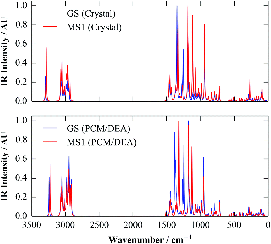Fig. 5 Simulated IR spectra for the GS and MS1 systems, calculated with the PBE functional. The top panel shows the spectra obtained from a periodic calculation on the two fully-optimised molecular crystals, while the lower panel shows the spectra from molecular calculations with a polarisable-continuum model using diethylamine as a solvent (DEA; ε_static = 3.6). The spectra were all broadened using a Lorentzian function with a full-width at half-maximum (FWHM) of 7.5 cm⁻¹.

The overall correspondence between the two sets of spectra is very good. Although there are minor variations in the calculated intensities, the spectra have similar overall forms, and most of the calculated peak positions are likewise very similar. The only notable exception is in the position of a pair of bands around ∼1400 cm⁻¹, which correspond to a mixture of vibrations of the isomerisable ligands and parts of the Et₄dien backbone, and which lie on top of each other in the periodic calculations, but are visibly separated in the continuum ones. This suggests a slight difference in the bonding of the ligand in the two sets of calculations, which may well be related to the small energy differences between the periodic and continuum calculations evident in Fig. 4.

It is also worth noting that, despite the use of the continuum model, as only a single molecule is present, the molecular calculations would not be able to reproduce phonon modes corresponding to collective motions of two or more of the four molecules in the crystallographic unit cell, which could potentially lead to discrepancies, in particular in the low-wavenumber (“fingerprint”) region of the spectra. The good correspondence between the periodic and molecular spectra in Fig. 5 therefore indicates that, to a very good approximation, the vibrational modes of the molecular crystal correlate with those of the molecular species, lending further support to the treatment of the molecules in the solid as independent entities.

Given the good performance of the continuum model with the calculated dielectric constant, we opted to compute IR and Raman spectra for both isomers with the more accurate M06 functional, which, as a hybrid functional, is in particular more likely to predict Raman polarisabilities more accurately than (meta-)GGAs. The calculated spectra are compared against room-temperature IR and Raman data collected from single crystals in Fig. 6.

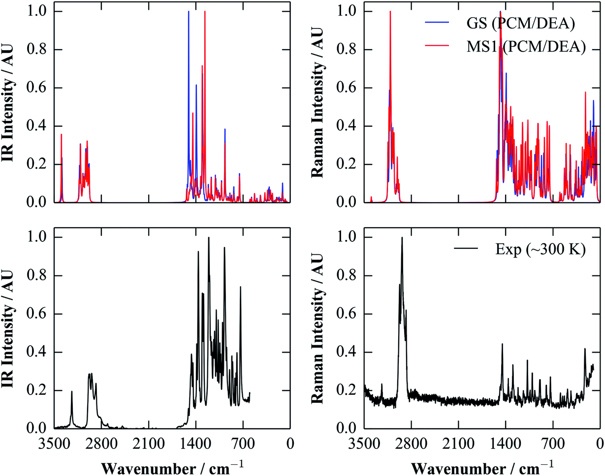Fig. 6 Simulated IR and Raman spectra of the GS (blue) and MS1 (red) molecules, compared to room-temperature (∼300 K) spectra taken from single crystals (black). The simulated spectra were obtained using the M06 functional and a polarisable continuum of diethylamine (DEA; ε_static = 3.6). As in Fig. 5, these spectra were broadened using a Lorentzian function with a full-width at half-maximum (FWHM) of 7.5 cm⁻¹.

There is a generally good correspondence between the simulated and experimental spectra. There are some notable mismatches in the predicted intensities, particularly in the case of the Raman spectra, although this could be due in part to the (arbitrary) choice of the broadening width for the calculated spectra. However, the positions of the peaks appear to be fairly well modelled, enabling assignment of some of the IR bands between ∼1000 and 1500 cm⁻¹ to the GS and MS1 isomers. This agreement nicely illustrates a potential utility of computation for supporting characterisation.

Optical properties

Optical properties arise from electronic excitations, and are a response property of the system. Modelling them formally requires solution of the time-dependent Schrödinger equation, or, more practically, modelling a perturbation to the ground-state electronic wavefunctions in response to an external field (e.g. as in the TD-DFT formalism).

The method implemented in VASP uses a perturbative linear-response method to obtain the frequency-dependent dielectric function, ε(E), which, in essence, entails an enumeration over transitions between filled and empty electronic states.⁷¹ From ε(E), various optical properties can be calculated, including refractive indices (n), extinction coefficients (κ), and absorption coefficients (α), the latter of which can be compared to experimentally-recorded UV-visible spectra. Fig. 7 compares these quantities for the GS and MS1 structures, computed from the TPSS-optimised crystal structures with a PBE0 ground-state reference.

Fig. 7 Optical properties of the GS (blue) and MS1 (red) isomers, computed from the TPSS-optimised crystal structures using a PBE0 ground-state reference. The plots compare the real (solid lines) and imaginary (dashed lines) parts of the frequency-dependent dielectric function ε(E), ε_r/ε_i, the refractive index, n, the extinction coefficient, κ, and the absorption coefficient, α. Each of the latter three plots are annotated with the equations used to calculate the quantities from ε(E).

The UV-visible spectrum of the GS molecular crystal published previously⁴⁶ does not extend into the deep UV, but the key features in the visible region are a long absorption tail around 400 nm, plus a second, broad isolated peak at ∼650 nm. The most likely comparison between this and the spectrum in Fig. 7 is that the absorption tail is blue-shifted by ∼200 nm, while the peak at 650 nm is not reproduced.

For comparison, we calculated spectra for the GS and MS1 molecules using the linear-response TD-DFT implemented in Gaussian. As for the calculations in the previous section, we used the M06 functional, together with a 6-311+G(d) basis set and a polarisable continuum of diethylamine. To compute the spectra, we analysed the 30 lowest-energy triplet transitions. The calculated spectra are shown in Fig. 8.

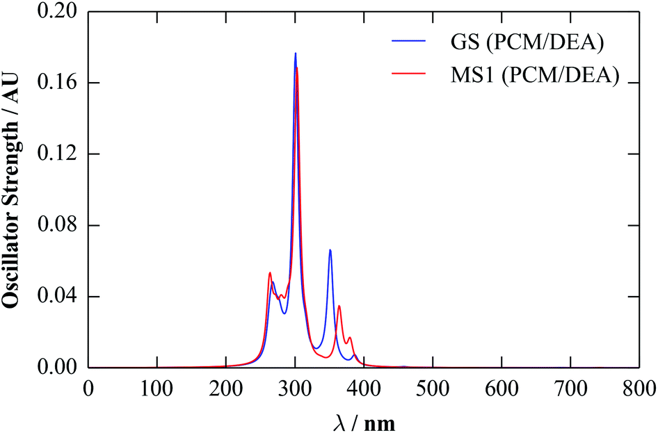Fig. 8 UV-visible spectra of the GS and MS1 molecules, calculated using linear-response TD-DFT with M06 and a polarisable continuum of diethylamine (DEA; ε_static = 3.6). The spectra have been broadened using a Lorentzian function with a full-width at half-maximum (FWHM) of 10 nm.

The overall structure of both spectra is similar to the 150–250 nm region of the solid-state one, consisting of primary high- and low-intensity peaks with some fine structure. The red shift of ∼200 nm compared to the periodic spectra suggests that the more sophisticated TD-DFT method implemented in the molecular code gives a better description of the optical-absorption profile, and the position of the absorption tail agrees much better with the experimental data.

Based on our previous calculations,⁴⁰ the majority of the transitions correspond to delocalised metal-to-ligand transitions, with large components on the Ni d orbitals, while the majority of the states from ∼450–350 nm can be assigned as metal-to-ligand charge-transfer bands. We note that, while the computational parameters used in these and in the present calculations are very similar, the continuum solvent used in the previous study (H₂O) has a considerably larger dielectric constant (ε_static = 80.1). However, we found that, while the positions of the absorption bands were sensitive to the dielectric constant, their nature and relative ordering were not, with the assignments being the same both in the gas phase and in a continuum of H₂O.

The broad peak at 650 nm is again not reproduced in these spectra. However, considering the individual calculated transitions (see ESI†), there are several states with lower excitation energies, but with negligible oscillator strengths. The orbitals involved have a significant Ni d component, suggesting them to be (symmetry forbidden) d–d transitions, which perhaps become weakly allowed when coupled to vibrations. This could, in principle, be modelled by performing TD-DFT calculations on structures displaced along the vibrational modes, although this is much more computationally demanding.

These results, and also those in our previous work,⁴⁰ suggest that further optimisation of the computational parameters may be required to reproduce accurately the experimental UV-visible spectra for this system. However, the superior performance of the continuum TD-DFT calculation over the periodic linear-response method highlights the potential benefits of being able to use molecular calculations, and their excited-state functionality, while accounting approximately for the influence of the crystalline environment.

4 Discussion and conclusions

The results in the previous section demonstrate quantitatively the performance of polarisable-continuum models in approximately accounting for the influence of the molecular crystal environment in molecular calculations on the component species. With well-converged basis sets, continuum calculations, in conjunction with dielectric constants obtained from periodic calculations, were able to reproduce a broad range of properties of the [Ni(Et₄dien)(η²-O,ON)(η¹-NO₂)] system, including energetics, vibrational frequencies, and, to a reasonable extent, optical properties. The correspondence between the continuum and periodic calculations was very good, and the comparison with available experimental data was also generally favourable. Moreover, and particularly with regard to modelling electronic excitations, the benefits of the higher levels of theory accessible in molecular calculations were clearly demonstrated.

The method explored in this work is fairly straightforward, and effectively combines some of the strengths of periodic and molecular calculations to allow for a more complete theoretical characterisation of molecular solids. For its broader applicability, the most important proviso is the assumption inherent in the polarisable-continuum approach, i.e. that the interactions between the molecular units in the solid are well represented by a dielectric-screening effect. It remains to be discussed, however, for which sorts of system this is a good approximation, and for which systems it should be expected to fail, e.g. crystals with longer-range intermolecular interactions such as π-stacking. For systems where this method works well, however, we anticipate that theoretical calculations should be a valuable tool for modelling and understanding a broad spectrum of state-of-the-art experimental work.

While the main focus of this study has been on the methodology, the calculations also provide some interesting insight into the chemistry of [Ni(Et₄dien)(η²-O,ON)(η¹-NO₂)], reinforcing the findings of our previous study.⁴⁰ It is quite clear that the crystalline environment significantly influences the relative stabilities of the different linkage isomers, in this case increasing the energy difference between the GS and MS1 forms relative to the gas phase. To explore this further, as a theoretical exercise we calculated the GS-MS1 energy difference using COSMO for a range of dielectric constants, spanning the two-orders-of-magnitude range covered by common solvents (Fig. 9).

Fig. 9 Dependence of the GS-MS1 energy difference on the dielectric constant, ε_static, of the medium. The shaded region corresponds to values between 3 and 4, which is the range computed for [Ni(Et₄dien)(η²-O,ON)(η¹-NO₂)]. Points outside of this range are annotated with solvents with comparable values of ε_static. All values were computed with the M06 functional, according to the same procedure used to obtain the values in Fig. 4.

This plot clearly illustrates that, by hypothetically tuning the dielectric constant of the crystal, the energy difference between the two isomers can be adjusted over quite a large range. In general, a stronger dielectric screening appears to increase the energy difference, with the effect saturating beyond values of ε_static around 30. Up to this limit, however, there is potentially scope for controlling the kinetics of the isomerisation process through the chemistry of the molecular species. This adds a new perspective to the established practice of using crystal engineering to create a “reaction cavity” for the isomerisation to occur within.^39,40,43,51

To investigate this finding in more detail, it would be interesting to calculate the dielectric constants of other known Ni–NO₂ linkage-isomer systems, and to relate these to the photoconversion yield and/or the presence or absence of thermal–isomerisation pathways. It may perhaps also be of interest to relate the dielectric constant to other properties, such as the optical-absorption profile, and the energy difference between magnetic configurations.

To conclude, polarisable-continuum models represent an effective means of including the influence of the crystalline environment in molecular calculations on the [Ni(Et₄dien)(η²-O,ON)(η¹-NO₂)] system. We have compared quantitatively a number of properties, and observed good overall agreement both with periodic calculations and experimental data, as well as obtaining new insight into the properties of this system, in particular the effect of the dielectric environment on the linkage isomerism. This work represents a step towards developing more general approaches to the theoretical characterisation of molecular solids, and, ultimately, to working on more complex topics, such as performing high-level electronic-structure calculations and exploring excited-state potential-energy surfaces.

Acknowledgements

The authors would like to thank Mr Richard Driscoll for his assistance with collecting Raman spectra of [Ni(Et₄dien)(η²-O,ON)(η¹-NO₂)]. The authors gratefully acknowledge financial support from an EPSRC programme grant (Grant no. EP/K004956/1) and the European Research Council (Grant no. 277757). We acknowledge use of the HECToR and ARCHER supercomputers through membership of the UK HPC Materials Chemistry Consortium, which is funded by EPSRC Grant no. EP/F067496, in the completion of this work.

References

1. J. P. Perdew and K. Schmidt, Jacob’s ladder of density functional approximations for the exchange-correlation energy, Antwerp, Belgium, 2001.
2. P. Hohenberg and W. Kohn, Phys. Rev. [Sect.] B, 1964, 136, 864–871.
3. W. Kohn and L. J. Sham, Phys. Rev., 1965, 140, 1133–1138.
4. L. Hedin, Phys. Rev., 1965, 139, A796–A823.
5. C. Moller and M. S. Plesset, Phys. Rev., 1934, 46, 0618–0622.
6. J. Čížek, J. Chem. Phys., 1966, 45, 4256–4266.
7. J. M. Skelton, S. C. Parker, A. Togo, I. Tanaka and A. Walsh, Phys. Rev. B: Condens. Matter Mater. Phys., 2014, 89, 205203.
8. J. Tomasi, B. Mennucci and R. Cammi, Chem. Rev., 2005, 105, 2999–3093.
9. A. Klamt and G. Schuurmann, J. Chem. Soc., Perkin Trans. 2, 1993, 799–805.
10. A. M. Reilly, D. A. Wann, M. J. Gutmann, M. Jura, C. A. Morrison and D. W. H. Rankin, J. Appl. Crystallogr., 2013, 46, 656–662.
11. D. M. S. Martins, D. S. Middlemiss, C. R. Pulham, C. C. Wilson, M. T. Weller, P. F. Henry, N. Shankland, K. Shankland, W. G. Marshall, R. M. Ibberson, K. Knight, S. Moggach, M. Brunelli and C. A. Morrison, J. Am. Chem. Soc., 2009, 131, 3884–3893.
12. S. Hunter, T. Sutinen, S. F. Parker, C. A. Morrison, D. M. Williamson, S. Thompson, P. J. Gould and C. R. Pulham, J. Phys. Chem. C, 2013, 117, 8062–8071.
13. J. Binns, M. R. Healy, S. Parsons and C. A. Morrison, Acta Crystallogr., Sect. B: Struct. Sci., Cryst. Eng. Mater., 2014, 70, 259–267.
14. S. Hirata, K. Gilliard, X. He, J. Li and O. Sode, Acc. Chem. Res., 2014.
15. R. A. DiStasio, O. A. von Lilienfeld and A. Tkatchenko, Proc. Natl. Acad. Sci. U. S. A., 2012, 109, 14791–14795.
16. R. A. DiStasio, V. V. Gobre and A. Tkatchenko, J. Phys.: Condens. Matter, 2014, 26.
17. S. Grimme, J. Comput. Chem., 2006, 27, 1787–1799.
18. S. Grimme, J. Antony, S. Ehrlich and H. Krieg, J. Chem. Phys., 2010, 132.
19. A. Tkatchenko and M. Scheffler, Phys. Rev. Lett., 2009, 102.
20. A. Tkatchenko, R. A. DiStasio, R. Car and M. Scheffler, Phys. Rev. Lett., 2012, 108.
21. M. Dion, H. Rydberg, E. Schroder, D. C. Langreth and B. I. Lundqvist, Phys. Rev. Lett., 2004, 92.
22. K. Lee, E. D. Murray, L. Z. Kong, B. I. Lundqvist and D. C. Langreth, Phys. Rev. B: Condens. Matter Mater. Phys., 2010, 82.
23. P. Cudazzo, M. Gatti and A. Rubio, Phys. Rev. B: Condens. Matter Mater. Phys., 2012, 86.
24. T. A. Wesolowski and A. Warshel, J. Phys. Chem., 1993, 97, 8050–8053.
25. T. Wesolowski, R. P. Muller and A. Warshel, J. Phys. Chem., 1996, 100, 15444–15449.
26. H. P. Hratchian, P. V. Parandekar, K. Raghavachari, M. J. Frisch and T. Vreven, J. Chem. Phys., 2008, 128.
27. P. V. Parandekar, H. P. Hratchian and K. Raghavachari, J. Chem. Phys., 2008, 129.
28. V. Bezugly and U. Birkenheuer, Chem. Phys. Lett., 2004, 399, 57–61.
29. C. Willnauer and U. Birkenheuer, J. Chem. Phys., 2004, 120, 11910–11918.
30. S. H. Wen, K. Nanda, Y. H. Huang and G. J. O. Beran, Phys. Chem. Chem. Phys., 2012, 14, 7578–7590.
31. O. Bludsky, M. Rubes and P. Soldan, Phys. Rev. B: Condens. Matter Mater. Phys., 2008, 77.
32. M. A. Kochman, A. Bil and C. A. Morrison, Phys. Chem. Chem. Phys., 2013, 15, 10803–10816.
33. C. P. Kelly, C. J. Cramer and D. G. Truhlar, J. Chem. Theory Comput., 2005, 1, 1133–1152.
34. T. N. Truong, J. Phys. Chem. B, 1998, 102, 7877–7881.
35. F. P. Cossio, G. Roa, B. Lecea and J. M. Ugalde, J. Am. Chem. Soc., 1995, 117, 12306–12313.
36. R. M. Jackson and M. J. E. Sternberg, J. Mol. Biol., 1995, 250, 258–275.
37. R. Cammi, B. Mennucci and J. Tomasi, J. Phys. Chem. A, 2000, 104, 5631–5637.
38. G. Scalmani, M. J. Frisch, B. Mennucci, J. Tomasi, R. Cammi and V. Barone, J. Chem. Phys., 2006, 124.
39. M. R. Warren, T. L. Easun, S. K. Brayshaw, R. J. Deeth, M. W. George, A. L. Johnson, S. Schiffers, S. J. Teat, A. J. Warren, J. E. Warren, C. C. Wilson, C. H. Woodall and P. R. Raithby, Chem.–Eur. J., 2014, 20, 5468–5477.
40. J. M. Skelton, R. Crespo-Otero, L. E. Hatcher, S. Parker, P. Raithby and A. Walsh, CrystEngComm, 2015, 17, 383–394.
41. L. E. Hatcher and P. R. Raithby, Coord. Chem. Rev., 2014, 277–278, 69–79.
42. M. D. Carducci, M. R. Pressprich and P. Coppens, J. Am. Chem. Soc., 1997, 119, 2669–2678.
43. M. R. Warren, S. K. Brayshaw, A. L. Johnson, S. Schiffers, P. R. Raithby, T. L. Easun, M. W. George, J. E. Warren and S. J. Teat, Angew. Chem., 2009, 121, 5821–5824.
44. L. E. Hatcher, M. R. Warren, D. R. Allan, S. K. Brayshaw, A. L. Johnson, S. Fuertes, S. Schiffers, A. J. Stevenson, S. J. Teat, C. H. Woodall and P. R. Raithby, Angew. Chem., Int. Ed., 2011, 50, 8371–8374.
45. S. K. Brayshaw, T. L. Easun, M. W. George, A. M. E. Griffin, A. L. Johnson, P. R. Raithby, T. L. Savarese, S. Schiffers, J. E. Warren, M. R. Warren and S. J. Teat, Dalton Trans., 2012, 41, 90–97.
46. L. E. Hatcher, J. Christensen, M. L. Hamilton, J. Trincao, D. R. Allan, M. R. Warren, I. P. Clarke, M. Towrie, D. S. Fuertes, C. C. Wilson, C. H. Woodall and P. R. Raithby, Chem.–Eur. J., 2014, 20(11), 3128–3134.
47. P. Coppens, I. Novozhilova and A. Kovalevsky, Chem. Rev., 2002, 102, 861–883.
48. D. A. Johnson and V. C. Dew, Inorg. Chem., 1979, 18, 3273–3274.
49. A. Y. Kovalevsky, K. A. Bagley and P. Coppens, J. Am. Chem. Soc., 2002, 124, 9241–9248.
50. A. Y. Kovalevsky, K. A. Bagley, J. M. Cole and P. Coppens, Inorg. Chem., 2003, 42, 140–147.
51. A. E. Phillips, J. M. Cole, T. d'Almeida and K. S. Low, Phys. Rev. B: Condens. Matter Mater. Phys., 2010, 82, 155118.
52. S. K. Brayshaw, J. W. Knight, P. R. Raithby, T. L. Savarese, S. Schiffers, S. J. Teat, J. E. Warren and M. R. Warren, J. Appl. Crystallogr., 2010, 43, 337–340.
53. D. Schaniel, N. Mockus, T. Woike, A. Klein, D. Sheptyakov, T. Todorova and B. Delley, Phys. Chem. Chem. Phys., 2010, 12, 6171–6178.
54. Z. Tahri, R. Lepski, K.-Y. Hsieh, E.-E. Bendeif, S. Pillet, P. Durand, T. Woike and D. Schaniel, Phys. Chem. Chem. Phys., 2012, 14, 3775–3781.
55. B. Cormary, S. Ladeira, K. Jacob, P. G. Lacroix, T. Woike, D. Schaniel and I. Malfant, Inorg. Chem., 2012, 51, 7492–7501.
56. G. Kresse and J. Hafner, Phys. Rev. B: Condens. Matter Mater. Phys., 1993, 47.
57. P. E. Blochl, Phys. Rev. B: Condens. Matter Mater. Phys., 1994, 50, 17953–17979.
58. G. Kresse and D. Joubert, Phys. Rev. B: Condens. Matter Mater. Phys., 1999, 59.
59. J. P. Perdew, K. Burke and M. Ernzerhof, Phys. Rev. Lett., 1996, 77, 3865–3868.
60. L. A. Constantin, J. M. Pitarke, J. F. Dobson, A. Garcia-Lekue and J. P. Perdew, Phys. Rev. Lett., 2008, 100.
61. J. M. Tao, J. P. Perdew, V. N. Staroverov and G. E. Scuseria, Phys. Rev. Lett., 2003, 91.
62. C. Adamo and V. Barone, J. Chem. Phys., 1999, 110, 6158–6170.
63. M. Valiev, E. J. Bylaska, N. Govind, K. Kowalski, T. P. Straatsma, H. J. J. Van Dam, D. Wang, J. Nieplocha, E. Apra, T. L. Windus and W. de Jong, Comput. Phys. Commun., 2010, 181, 1477–1489.
64. M. J. Frisch, G. W. Trucks, H. B. Schlegel, G. E. Scuseria, M. A. Robb, J. R. Cheeseman, G. Scalmani, V. Barone, B. Mennucci, G. A. Petersson, H. Nakatsuji, M. Caricato, X. Li, H. P. Hratchian, A. F. Izmaylov, J. Bloino, G. Zheng, J. L. Sonnenberg, M. Hada, M. Ehara, K. Toyota, R. Fukuda, J. Hasegawa, M. Ishida, T. Nakajima, Y. Honda, O. Kitao, H. Nakai, T. Vreven, J. A. Montgomery Jr, J. E. Peralta, F. Ogliaro, M. J. Bearpark, J. Heyd, E. N. Brothers, K. N. Kudin, V. N. Staroverov, R. Kobayashi, J. Normand, K. Raghavachari, A. P. Rendell, J. C. Burant, S. S. Iyengar, J. Tomasi, M. Cossi, N. Rega, N. J. Millam, M. Klene, J. E. Knox, J. B. Cross, V. Bakken, C. Adamo, J. Jaramillo, R. Gomperts, R. E. Stratmann, O. Yazyev, A. J. Austin, R. Cammi, C. Pomelli, J. W. Ochterski, R. L. Martin, K. Morokuma, V. G. Zakrzewski, G. A. Voth, P. Salvador, J. J. Dannenberg, S. Dapprich, A. D. Daniels, Ö. Farkas, J. B. Foresman, J. V. Ortiz, J. Cioslowski and D. J. Fox, Gaussian, Inc., Wallingford, CT, USA, 2009.
65. R. Ditchfield, W. J. Hehre and J. A. Pople, J. Chem. Phys., 1971, 54, 724–728.
66. T. H. Dunning, J. Chem. Phys., 1989, 90, 1007–1023.
67. P. J. Hay and W. R. Wadt, J. Chem. Phys., 1985, 82, 270–283.
68. Y. Zhao and D. G. Truhlar, Theor. Chem. Acc., 2008, 120, 215–241.
69. A. D. Becke, J. Chem. Phys., 1993, 98, 1372–1377.
70. R. A. Lunt, A. J. Jackson and A. Walsh, Chem. Phys. Lett., 2013, 586, 67–69.
71. M. Gajdos, K. Hummer, G. Kresse, J. Furthmuller and F. Bechstedt, Phys. Rev. B: Condens. Matter Mater. Phys., 2006, 73.

---

Footnote

† Electronic supplementary information (ESI) available: includes additional data from the parameter testing in Section 3, including the effect of different DFT functionals on molecular geometry and extended basis-set convergence results, plus the full dataset from the molecular TD-DFT calculation. See DOI: 10.1039/c4fd00168k

---