Modeling approaches to predict removal of trace organic compounds by ozone oxidation in potable reuse applications

Abstract

Realized and potential threats of water scarcity due in part to global climate change have increased the interest in potable reuse of municipal wastewater. Recalcitrant trace organic compounds (TOrCs), including pharmaceuticals and endocrine disrupting compounds in wastewater are often not efficiently removed by conventional wastewater treatment processes. Ozone application has been demonstrated to be a highly efficient oxidation process to attenuate TOrCs. However, operation of ozone oxidation can be challenging in wastewater due to variations in water quality that can impact critical control points through fluctuations in ozone demand/decay. Therefore, this study implemented three explanatory modeling techniques including multiple linear regression (MLR), artificial neutral network (ANN), and PC (principal component)-ANN to predict TOrCs removal by ozone oxidation in a secondary wastewater effluent. All the developed models displayed good agreements between the predicted TOrCs removal and the observed TOrCs removal with the explanatory variables (input variables) of ozone dose, total organic carbon (TOC) concentration, and rate constants of ozone and ˙OH. PC-ANN displayed the highest predictive power in the external validation step (R² = 0.934) successively followed by ANN (R² = 0.914) and MLR (R² = 0.758). Based on the MLR model equation and the result of sensitivity analysis of the ANN model, TOC was found to have negligible effects on the TOrCs removal in a given water quality. Despite the predictive power of the ANN model, possible overfitting remains to be solved since the cross validation coefficient (q²) value calculated by the leave-one-out cross validation was not sufficient to ensure model predictive power. In contrast, the PC-ANN model was found to be robust across the scenarios applied. This study provides a guideline for software sensors to control ozone treatment processes in regards to TOrC oxidation and likely can be adapted to monitor disinfection as well.

---

Water impact

Trace organic compounds (TOrCs) have increasingly drawn attention, particularly occurrence in wastewater effluents and subsequently for applications involving potable water reuse. Ozone oxidation has been demonstrated as an efficient process for transforming the majority of TOrCs and can be a viable treatment option for reuse applications. However, real-time online monitoring is nearly impossible at the moment because monitoring of TOrCs requires highly sensitive analytical techniques such as mass spectrometry. This paper presents several modeling approaches including multiple linear regression, an artificial neural network (ANN), and principal component (PC) combined with ANN (PC-ANN) in order to predict the removals of TOrCs in a secondary wastewater effluent. In addition, this paper attempted elucidating procedures to select a robust model for the prediction of TOrCs removal, eventually providing a guideline for the application of the implemented modeling techniques to real-time model-based software sensors.

1. Introduction

Water scarcity in many parts of the world has become increasingly severe and is anticipated to be more aggravated in the future.¹ In addition, global climate change is dynamically altering regional climates, thereby obscuring precise prediction and efficient management of natural water resources.² In order to provide a drought-proof source of fresh water, potable water reuse is being increasingly explored as a reliable water resource.³ This is particularly true in arid and semi-arid geographies where water reuse being employed to expand water resource portfolios.⁴

Engineered potable water reuse systems employ advanced treatment technologies and they can produce water with nearly any desired quality.⁵ However, the efficiency and efficacy of water treatment technologies is important to the continued acceptance and advancement of reuse of municipal wastewater for augmenting potable water supplies.⁶ Of key interest is the efficacious attenuation of chemical contaminants that are recalcitrant in conventional wastewater treatment technologies.⁷ Of the vast number of trace organic compounds (TOrCs) reported to occur in wastewater, bioactive and highly potent substances such as certain pharmaceuticals and endocrine disrupting compounds (EDCs) are a potential threat to ecological and public health.⁸

Thus most potable water reuse programs utilize a multi-barrier treatment regime.³ Advanced oxidation processes (AOPs) are often implemented in potable water reuse applications as powerful oxidants for transformation of many organic constituents^9,10 and for disinfection of essentially any biological organism.^11,12 For instance, ozone is a strong oxidant and has been well proven to remove majority of TOrCs with high efficacy.¹³ In water, ozone is readily decomposed, and OH radicals (˙OH) are formed in a chain reaction.¹⁴ Ozone is a selective oxidant that can rapidly react with electron-rich moieties (ERM) such as aromatic compounds, organosulfur compounds, and deprotonated amines, whereas ˙OH is relatively non-selective oxidant with high reactivity with the majority of organic structures.¹⁵

For an efficient operation of ozone treatment processes in reuse applications, the prediction of TOrC attenuation is valuable. In general, two kinds are modeling techniques can be considered for predictive treatment efficacy: deterministic models and numerical models. Recently, Lee et al. deterministically predicted TOrC removal in wastewater based on a kinetic equation as follows:

where [TOrC] and [TOrC]₀ refer to the concentrations of TOrC after and before ozone application, respectively; and where k_O3 and k_˙OH are the second-order reaction rate constants with ozone and ˙OH, respectively. For prediction of TOrCs attenuation using eqn (1), ozone and ˙OH exposures (i.e., ∫[O₃]dt and ∫[˙OH]dt, respectively) need to be determined using an ˙OH-probe compound, often p-chlorobenzoic acid (pCBA).¹⁶ This methodology is readily achieved in laboratory batch reactors; however, in water with high ozone consumption or low ozone to dissolved organic carbon (DOC) ratio, ozone is readily consumed instantaneously. TOrCs with high reactivity with both ozone and ˙OH, such as carbamazepine and sulfamethoxazole, can be rapidly oxidized during the first 20 sec of ozone exposure, therefore requiring a specifically designed apparatus such as a continuous quench-flow system to acquire accurate values of the ozone and ˙OH kinetics.¹⁷ In addition, the efficiency of TOrCs attenuation is highly dependent on the kinetics of ozone reaction with dissolved organic matter. In turn, seasonal variation of water quality (i.e., composition of dissolved organic matter) influences the extent of TOrCs attenuation by altering ozone and ˙OH exposures.

Numerical modeling techniques, particularly based on exploratory method, for the prediction of TOrCs attenuation in wastewater can have several benefits. For example, no apparatus is required to measure characteristics of ozone decomposition kinetics expressed by integral exposures of ozone and ˙OH. In addition, a generated or trained model based on actual data enables facile prediction of TOrCs under the seasonal variation of ozone decay/demand characteristics.

Hence, the objective of this study is to develop exploratory models to predict removal of TOrCs in a secondary wastewater quality by ozone processes. Multiple linear regression (MLR), and artificial neural network (ANN), and principal component (PC)-ANN models were developed and their predictive power and robustness were compared. A discussion regarding the internal and external validation is provided along with application of the developed models to software sensors.

2. Experimental

2.1. Pilot-scale ozone tests

Secondary wastewater effluent was collected at a 7500 m³ per day capacity wastewater treatment facility located in southern Arizona, USA. The wastewater treatment plant receives mainly domestic wastewater and consists of bar screens, aerated lagoons, percolation basins, biological nutrient removal ditch, and clarifiers partially returning sludge. The secondary wastewater was intercepted before chlorination and supplied to an ozone pilot plant (Xylem Wedeco Modular 8HC, Germany). Five sampling campaigns were conducted over 30 months with applied ozone doses ranging from 0.5 mg L⁻¹ to 9 mg L⁻¹.

2.2. Analytical methods and selection of TOrCs for model development

The models employed in this study are exploratory, thus an adequate amount of data needs to be used for reliable model generation/training. Twenty-nine TOrCs were monitored over the sampling campaigns but some were not consistently detected.¹⁸ Therefore, six compounds that had a 100% occurrence in the secondary wastewater effluents over the five sampling campaigns were used as indicators in the model development (Table 1). The selected six compounds indicate four relative levels of reactivity with ozone and ˙OH, and are thus binned into four groups.

Table 1 List of TOrCs selected for the model development

TOrC	Application	Structure	k O3,pH7 [M^−1 s^−1]	k ˙OH [M^−1 s^−1]	Ref.
Group I: high reactivity with both ozone and ˙OH kO3,pH7 > 1 × 10^5 M^−1 s^−1 and k˙OH > 5 × 10^9 M^−1 s^−1
Sulfamethoxazole	Antibiotics		5.7 × 10^5	8.5 × 10^9	19
Group II: moderate reactivity with ozone and high reactivity with ˙OH 10 < kO3,pH7 ≤ 1 × 10^5 M^−1 s^−1 and k˙OH > 5 × 10^9 M^−1 s^−1
Atenolol	β-blocker		2.0 × 10^3	8 × 10^9	11
Group III: low reactivity with ozone and high reactivity with ˙OH kO3,pH7 < 10 M^−1 s^−1 and k˙OH > 5 × 10^9 M^−1 s^−1
Ibuprofen	Nonsteroidal anti-inflammatory drug		9.6	7.4 × 10^9	20, 21
Primidone	Anticonvulsant		1	6.7 × 10^9	22
Group IV: low reactivity with ozone and moderate reactivity with ˙OH kO3,pH7 < 10 M^−1 s^−1 and 1 × 10^9 < k˙OH ≤ 5 × 10^9 M^−1 s^−1
DEET	Insect repellent		<10	5 × 10^9	23
Meprobamate	Anti anxiety drug		<1	3.7 × 10^9	24

---

The six representative TOrCs, as well as other TOrCs not included in the model development, were analyzed using a fully-automated online solid phase extraction (SPE) system (Flexcube-Agilent Technologies, Santa Clara, CA). This module was connected inline to a 1290 Agilent liquid chromatograph (LC) coupled to a tandem mass spectrometer (MS/MS-Agilent Technologies 6460). Method optimization parameters, reproducibility and sensitivity have been described previously.²⁵ Briefly, the method employed only 1.7 mL to active method detection limits between 0.4 and 3 ng L⁻¹ for the target analytes. The method used a PLRP-s (2.1 × 12.5 mm) online SPE cartridge for retention of target analytes and an Agilent Poroshell EC-120 C-18 (2.1 × 50 mm) column for gradient elution. The samples were spiked with a mixture of isotopically-labeled surrogate standards to account for matrix effects.

Total organic carbon (TOC) was measured using Shimadzu TOC-L CSH Total Organic Carbon Analyzer (Shimadzu Corp., Japan). Before analysis, samples were acidified to pH 3 or lower using HCl (ACS grade, 37%, Sigma Aldrich).

2.3. Modeling procedure

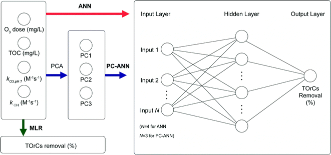
Three exploratory models were employed to predict removal of TOrCs in a secondary wastewater effluent: MLR, ANN, and PC-ANN. Fig. 1 depicts the flow diagram of the modeling procedure. For MLR and ANN, total organic carbon (TOC), applied ozone dose (in mg L⁻¹), rate constants of O₃ and ˙OH for the six TOrCs were used as explanatory variables. PCA was conducted to transform the four explanatory variables to linearly independent variables (i.e., PC scores) which are used for explanatory variables for PC-ANN. Data sets from the first four sampling campaigns were used for the model generation/training step and a data set from the last sampling campaign was used for the external validation step. All the model calculations were conducted using MATLAB 2014b (The MathWorks Inc., Natick, MA).

Fig. 1 Flow diagram of the modeling procedure.

2.3.1. MLR. MLR is a linear regression method for multiple explanatory variables and can be developed as follows:where x_i is the explanatory variable of i (or independent variable), y is the dependent variable, β_i is the regression coefficient, and ε is the residual.

2.3.2 ANN. ANN is a computational model made up of a number of simple and interconnected processing elements (i.e., neurons).²⁶ This technique is widely applied to predict occurrences of contaminants in natural water systems and removals of contaminants in complicated treatment processes.^27–29 ANN consists of input, hidden, and output layers. In this study, eight hidden layer nodes were employed since the optimal number of hidden layer nodes is generally twice the number of input and output layer nodes.³⁰ A two-layered feed-forward neural network with Levenberg–Marquardt algorithm was used for the training. A sigmoidal transfer function was implemented for the transfer of information between the layers. The data sets were randomly divided into 70%, 15%, and 15% for training, validation, and testing.

2.3.3. PC-ANN. A PC-ANN model was constructed to compare with the ANN model to incorporate model robustness. PC-ANN consolidates PCA with ANN, with the main benefit of PC-ANN ability to resolve collinearity among explanatory variables.³¹ Three principal components (PCs) as input variables (explanatory variables) were chosen since 100% of the cumulative percentage of the explained variations by three PCs was achieved. The other modeling procedure of PC-ANN is the same as described in the preceding section except that six hidden layer nodes were used due to the reduced number of the explanatory variables.

2.3.4. Internal and external validation. Validation plays crucial roles in modeling, particularly for exploratory models in order to ensure robustness and predictive power. The validation procedure generally consists of two types: internal validation and external validation. Internal validation is a statistical diagnostic to check the predictive ability of models. In this study, a leave-one-out (LOO) cross validation method was employed and a cross-validated correlation coefficient (q²), an evaluation criterion of model predictive power, can be calculated as follows:³²where y_i, ŷ_i, and are the observed, predicted and averaged values of the dependent variables, respectively.

2.3.5. Sensitivity analysis. Exploratory models including ANN and PC-ANN can possibly be over-fitted. Sensitivity analysis helps in meaningful interpretation of developed models by relatively comparing the sensitivity indices of each explanatory variable.³³ In general, over-fitted models are not physically interpretable. Hence, the implementation of sensitivity analysis can alleviate possibilities of overfitting. Latin Hypercube-One-factor-At-a-Time (LH-OAT), a global sensitivity analysis, was implemented to elucidate the relative impacts of each explanatory variable on TOrCs removal.³⁴ The detailed procedure of the LH-OAT method is described in ESI.†

3. Results and discussion

3.1. Occurrence of TOrCs

Fig. 2 shows the occurrence data of TOC and TOrCs used in this study. The mean TOC value of the secondary wastewater effluent over the sampling campaigns is ~6 mg L⁻¹ and its coefficient of variation (CV) is 15.4%. Compared to the variation of TOC, the variation of TOrCs was higher. All the TOrCs showed variation greater than 20%, except for meprobamate. In general, the occurrence and concentrations of TOrCs are considered highly seasonally dependent.^35,36 TOrCs considered in this study are anthropogenically driven and their occurrences are dependent on their usage/consumption. For instance, highly frequent detection of sulfamethoxaolze in many countries was attributed to its high usage.³⁷ Sulfamethoxazole is highly soluble at neutral pH (log D_ow = −0.05 at pH 7, calculated using MarvinSketch 15.2.16.0, ChemAxon Ltd.) and it is not likely to be adsorbed onto sludges. Meanwhile, enzymatic reaction may be a factor of seasonal variation of sulfamethoxazole under the depletion of biodegradable carbon and nitrogen sources available.³⁸ Ibuprofen and DEET showed higher variation than the others. Ibuprofen is amenable to biodegradation, hence it is reasonable that the seasonal variation can be partially due to the seasonal change in biodegradation efficiency as well as its variation of usage.³⁹ It is noteworthy that the variation of DEET may be due to possible presence of mimic compounds, that provide a false-positive signal, as reported in a recent study.⁴⁰

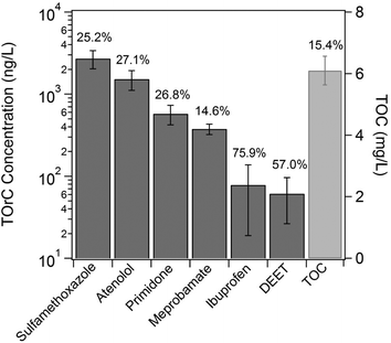Fig. 2 The occurrence of the TOrCs selected for modeling and TOC. Error bars indicate the standard deviations of each TOrC and TOC.

3.2. Modeling results of MLR and ANN and their comparison

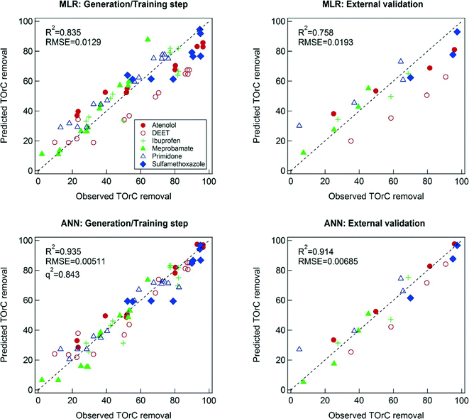
MLR shows a relatively good agreement between the predicted and observed TOrC removal (Fig. 3). One of the key assumptions of MLR is that the residual error follows a normal distribution.⁴¹ To check normality of the residuals within the developed MLR model, a normal probability plot and a normality test based on Kolmogorov–Smirnov (KS) was conducted as shown in Fig. S1 (ESI†). The p-value from the normality test (<0.05) indicates that the KS test rejects the null hypothesis that the residuals of the model are drawn from a normal distribution at the 5% significant level. Transformations of the dependent variables (i.e., TOrCs removal) including log and square-root transformations did not help the residuals become normally distributed. So, the original form of the dependent variables was adopted for the modeling. It should be noted that the developed MLR model showed a good agreement between the predicted TOrCs removal and the observed one in the external validation, therefore the MRL model was considered reliable.

Fig. 3 Comparison of the predicted TOrCs removal with the observed TOrCs removal for the generation/training step and the external validation step of MLR and ANN. RMSE refers to the root-mean-square error.

MLR is considered a transparent model since the model can express the relation between explanatory variables and output variables mathematically.⁴² This feature of MLR enables physically meaningful interpretations of modeling result. The regression equation obtained by MLR is as follows:

Removal (%) = −32.77 + 10.22C_O3 + 1.130TOC + 6.912 × 10⁻⁵k_O3,TOrC + 6.023 × 10⁻⁹k_˙OH,TOrC. (4)

The estimated coefficient of C_O3 is 10.56, which indicates that the increment of 1 mg L⁻¹ ozone dose can achieve ~10% more TOrCs removal regardless of the type of TOrCs within the given water quality. It is obvious from this result an increase in ozone dose increases TOrCs removal. However, the positive value of estimated coefficient of TOC cannot physically explain TOrCs removal, which indicates that the increase in TOC can cause higher TOrCs removal. This physically non-interpretable result can be an indicator of failure in model development. In MLR modeling, statistical significances of the each regression coefficient need to be checked. That is, the null hypothesis that a regression coefficient is equal to zero needs to be tested. Table S1 in the ESI† shows the result of significance test. The p-value of the regression coefficient of TOC greater than 0.05 indicates that the coefficient is statistically equal to zero. In addition, the standard deviation of TOC in all the sampling campaigns was less than 1 mg L⁻¹ (Fig. 2), which means that the change in TOrC removal due to TOC estimated by MLR is ~1% in the variation of the given water quality (i.e., 1.012 × 1 mg L⁻¹). Therefore, the exclusion of TOC from the MLR model is necessary and a new MLR equation was obtained as follows:

Removal (%) = −25.93 + 10.27C_O3 + 6.900 × 10⁻⁵k_O3,TOrC + 6.052 × 10⁻⁹k_˙OH,TOrC. (5)

The regression result of the three-parameter MLR model is tabulated in the ESI† (Table S1). The values of regressions coefficients remain similar with eqn (3), which again indicates that TOC does not significantly influence the estimated TOrCs removal. One interesting aspect of the model is that the model linearly depends on the ozone concentration and rate constants of each TOrC. Since each TOrC has a unique rate constant, the removal is thoroughly reliant on the ozone dose in a linear manner. According to the data shown in Lee et al.'s work,²⁴ meprobamate and DEET (Group IV, compounds with low reactivity with ozone and moderate reactivity with ˙OH) showed relatively linear trends of their removals with respect to O₃/DOC (O₃ dose normalized by dissolved organic carbon concentration in mg/mg) whereas the TOrCs with high reactivity with ozone and ˙OH displayed logarithmic trends with respect to O₃/DOC. This non-linear trend of the TOrCs with relatively higher reactivity with ozone and ˙OH cannot be explained by the MLR model and may provoke relatively small deviation of the MLR model from the observed data. In addition, the fact that MLR model does not include the effects of TOC on TOrCs removal may also influence the predictability of the model. DOC (the dissolved fraction of TOC) is a key factor for ozone decomposition in water since DOC concentration and composition affects the ozone decomposition.⁴³ Therefore, complete exclusion of DOC may lower the predictive power of MLR.

Compared to MLR, the ANN resulted in better predictability of TOrC removal, with R² = 0.935 and 0.914 for the training and the external validation, respectively. Hidden neurons of ANN enable the prediction of nonlinear relation between explanatory variables and output variables.⁴⁴ However, this modeling technique is often considered as a “black box” and requires careful investigation of overfitting.⁴⁵ One of the most important criteria of models is their reproducibility in a domain of interest. Overfitting would cause inaccurate prediction although high goodness of fit can be achieved for a model training step. This study employed the data sets from four sampling campaigns for the model training step and the other data set from a sampling campaign for the external validation step. The data set for the external validation step can be considered independent on the data sets used in the model training step. Hence, the external validation can verify the reproducibility of the ANN model. In addition, the q² value from LOO cross validation procedure for the ANN model has higher value (i.e., 0.843) as shown in Fig. 3. High values of q² generally indicate predictive powers of models and q² > 0.5 is considered as good and q² > 0.9 as excellent.⁴⁶

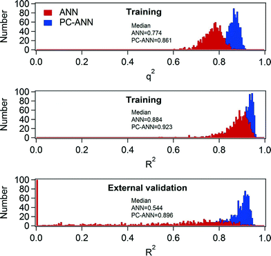
There are several cases addressing insufficiency of q² to ensure model predictive power.^47–49 As mentioned earlier, MLR can provide physically meaningful interpretation from the obtained model equation. Like MLR, ANN also can give insightful interpretation using a sensitivity analysis. LH-OAT sensitivity analysis method can provide relative effects of model input parameters on output variables. Two ANN models were selected to explain an overfitting problem that can be arisen during training procedures. One is the ANN model shown in Fig. 3 as an exemplary model with high goodness of fit for the both training and external validation step (Case 1). The other ANN model chosen (Case 2) has a high goodness of fit for the model training procedure, but with extremely low coefficient of determination (zero) in the external validation. Fig. 4 shows the sensitivity indices of the each explanatory variable for the two model cases. Case 1 showed an agreement with the modeling result of MLR. That is, TOC has minimal impacts on the TOrCs removal while ozone dose plays significant roles. The effects of k_O3 and k_˙OH are also relatively significant, which implies that each TOrC removal relies on oxidation kinetics. It was also found that the effects of k_˙OH is slightly more significant than k_O3. On the other hand, the most influential explanatory variable in Case 2 was TOC, which may be an indicator of overfitting. Hence, it is noteworthy that q² value would not sufficient to appreciate a predictive power for the used data sets. The more detailed investigation is made in the following section.

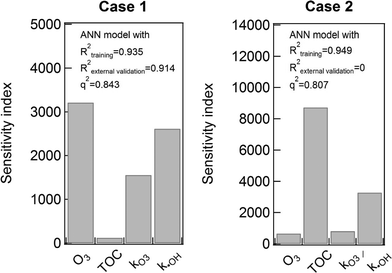Fig. 4 The result of LH-OAT sensitivity analysis of the two ANN models. The model selected for Case 1 was the one shown Fig. 3. Case 1 showed high R² values of both the training and external validation steps as well as high q² value. The model chosen for Case 2 was one with high a R² value for the training step, but zero value of R² for the external validation step.

3.3. Collinearity problem of ANN and the robustness of PC-ANN

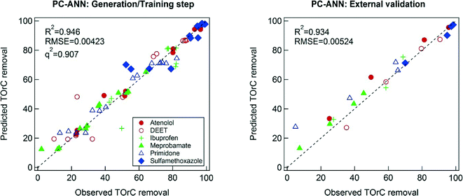
A necessary criterion to check the predictive power of the model in ANN is the q² value. However, Golbraikh and Tropsha found that a high q² value is necessary to develop a model with high predictability, but not sufficient to ensure the predictive power.⁵⁰ In this study, training data subsets and the initial weight of ANN were randomly selected, a reason that Case 1 and Case 2 have the different predictive power even though the same modeling technique was implemented. The randomized training data subsets and the initial weights can vary, either enhance or jeopardize, the predictive power of model. Robust modeling techniques should be reproducible and be validated in any condition. However, Case 2 clearly showed that the implemented ANN technique possibly provokes overfitting, thereby failing accurate prediction. Therefore, 1000 times model training steps with different (random) allocation of training data subsets and initial weight were conducted to elucidate the extent of robustness. In Fig. 5, the median values of R² and q² distributions of the ANN models are 0.884 and 0.774, respectively. However, the median value of R² for the external validation exhibited a relatively low value (0.544). Furthermore, ~10% of R² values among the 1000 times simulations were zero. Therefore, the ANN technique with the given explanatory data sets needs careful appreciations of its robustness. One important aspect is that the internal validation based on the LOO cross validation was found to be a necessary procedure, but not sufficient one for the prediction TOrCs removal by the ANN modeling technique. This may be due to collinearity of the explanatory variables. In the earlier section, both the MLR model equation and the sensitivity analysis of the ANN model displayed the negligible effects of TOC on the TOrCs removal. However, TOC may affect predictability of models because of its influence on ozone decay and ˙OH formation. In turn, there may be correlation between TOC and the other explanatory variables (i.e., collinearity).⁵¹ In that case, collinearity can be reduced by applying to PCA to ANN (i.e., PC-ANN).

Fig. 5 The distribution of q², R² for the model generation/training and R² for the external validation of ANN and PC-ANN. The vertical axis indicates the number of the simulations at the corresponding q² and R² values.

As depicted in Fig. 6, PC-ANN yielded excellent agreements between the predicted and observed TOrC removal for both the model training and external validation steps. When applying the same procedure with the ANN modeling for the evaluation of robustness, PC-ANN showed slightly better R² and q² values for the model training step as shown in Fig. 5. Moreover, the distribution of R² for the external validation showed that the PC-ANN modeling technique induced excellent predictive power even for the external validation step (the median value is 0.896), which implies that the explanatory variables would have collinearity in particular between ozone and TOC. Organic carbon is often considered when using O₃/DOC ratio as an operating parameter of ozone oxidation, which needs to be reflected during the modeling procedure.²⁴ Hence, a possible reason of better robustness of PC-ANN compared to ANN was that the PCA reduced the dimensionality (i.e., the number of explanatory variables) while eliminating collinearity between the explanatory variables.

Fig. 6 Comparison of the predicted TOrCs removal with the observed TOrCs removal for the generation/training step and the external validation step of PC-ANN. RMSE refers to the root-mean-square error.

3.4. Application of the developed models in an ozone pilot plant

There are pros and cons of the each exploratory models employed in this study. MLR model provides a model equation that can be interpreted in a physical manner. Due to the limitation of linearity of the model like other general linear models; however, it may not be proper to elucidate nonlinear removal trends of TOrCs with high reactivity with ozone and ˙OH. Compared to MLR, ANN displayed better predictive power in the ozonation process for TOrCs removal. However, ANN like other black box models cannot directly provide physically meaningful interpretation and has the serious possibility of overfitting. Internal validation based on LOO cross validation was not sufficient to appreciate the robustness of the ANN model, implying that the external validation procedure is inevitable. PC-ANN showed the highest predictive power among the applied exploratory models while maintaining reproducibility.

In a real ozone facility, the optimal operation of ozone oxidation processes is crucial since it can reduce operational cost and maximize the removal efficacy of TOrCs, hence providing a safe barrier of TOrCs in potable reuse applications. To this end, the best practice would be to apply online sensors to directly measure, or predict, TOrCs attenuation. Recently, the correlation of TOrCs removal with surrogate indicators such as spectroscopic parameters including UV absorbance at 254 nm and total fluorescence (i.e., the integral of fluorescence intensity over the excitation and emission wavelengths) was extensively studied in physico-chemical processes such as activated carbon adsorption and advanced oxidation processes.^11,52,53 These approaches would be practical and useful in a real plant since spectroscopic sensors require minimal pretreatment, accompany high frequency of data collection, and possess high sensitivity.⁵⁴ However, although these approaches possess such benefits, they cannot be mechanistically interpreted.⁵⁵ Therefore, the employment of multiple sensing techniques can lower possibilities of sensor failures and software sensor can support such analytical monitoring techniques for the prediction of TOrCs attenuation by ozonation. To this end, advantages and disadvantages of the three models employed in this study need to be elucidated.

Four input parameters including TOC, applied ozone dose, rate constants of O₃ and ˙OH of TOrCs of interest are necessary for the developments of models. Due to the inherent nature of exploratory modeling approaches in which models are built based upon data, regular monitoring of TOrCs is essential for building a robust model along with online TOC sensors. For the selection of a TOC sensor, chemical-based sensors such as catalytic combustion and UV/persulfate oxidation types would be recommended rather than optical-based TOC sensors since optical-based TOC sensors potentially display a bias of TOC measurement in oxidation processes.⁵⁶ A benefit of MLR is intuitive and easily understandable, so may be preferred for software sensor applications. In addition, the minimal influence of TOC on the model prediction enables the exclusion of TOC as an input parameter, which does not require implementation of TOC sensors. ANN displayed a good predictive power, but it may not be suitable for software sensor applications because a developed model can be overfitted, thereby losing its predictive power. In addition, internal validation such as LOO cross validation method cannot ensure the robustness of a model. PC-ANN could predict the TOrCs with high predictive power and showed its robustness, thereby capable of a precise software sensing technique. In addition, possible reductions in noise of data by PCA can enhance the predictability of highly nonlinear data, which renders the modeling technique more attractive for the TOrCs whose analysis is sensitive and possibly variable.

4. Conclusions

In this study, three explanatory modeling techniques including MLR, ANN, and PC-ANN were applied to predict TOrCs removal by ozone oxidation in a secondary wastewater effluent. All the developed models displayed good agreements between the predicted TOrCs removal and the observed TOrCs removal. The main findings in this study are summarized as follows.

- MLR model showed relatively good predictive power (R² values for the model generation and external validation were 0.835 and 0.758, respectively). Based on the model equation from the MLR, the effects of TOC was found to be negligible for the given water qualities.

- Better predictive power was achieved by ANN than MLR (R² values for the training and external validation were 0.935 and 0.914, respectively). However, the careful appreciation is required to avoid overfitting since the cross validation coefficient (q²) as an general indicator of predictive power of model by LOO cross validation was not sufficient to ensure model predictabilities.

- PC-ANN was displayed the highest predictability (R² values for the training and external validation were 0.946 and 0.934, respectively) among the three models while maintaining robustness confirmed by external validations.

The each implemented model accompanies pros and cons and can be flexibly applied to various software sensors with regard to aims of operation. Therefore, this study is expected to contribute to helping the real-time optimization of ozone dose in terms of TOrCs removal.

Acknowledgements

The authors would like to appreciate the operators at the wastewater treatment plant for their assistance in sample collection. We also thank Dr. Sylvain Merel in University of Tübingen, Germany for fruitful discussion on TOrCs analysis. We especially wish to acknowledge Jens Scheideler from Xylem Wedeco for providing the ozone pilot facility and related technical support. We also appreciate Agilent Technologies for help with acquisition and maintenance of the instrumentation used in this study.

References

1. M. Park, J. Lee, C. Boo, S. Hong, S. A. Snyder and J. H. Kim, Desalination, 2013, 314, 115–123.
2. N. V. Paranychianakis, M. Salgot, S. A. Snyder and A. N. Angelakis, Crit. Rev. Environ. Sci. Technol., 2014, 45, 1409–1468.
3. A. N. Pisarenko, B. D. Stanford, D. Yan, D. Gerrity and S. A. Snyder, Water Res., 2012, 46, 316–326.
4. D. Gerrity, B. Pecson, R. S. Trussell and R. R. Trussell, J. Water Supply: Res. Technol.--AQUA, 2013, 62, 321–338.
5. T. Asano and A. D. Levine, Water Sci. Technol., 1996, 33, 1–14.
6. S. A. Snyder, Ozone: Sci. Eng., 2008, 30, 65–69.
7. D. Gerrity, B. D. Stanford, R. A. Trenholm and S. A. Snyder, Water Res., 2010, 44, 493–504.
8. S. D. Kim, J. Cho, I. S. Kim, B. J. Vanderford and S. A. Snyder, Water Res., 2007, 41, 1013–1021.
9. F. L. Rosario-Ortiz, E. C. Wert and S. A. Snyder, Water Res., 2010, 44, 1440–1448.
10. D. Gerrity and S. A. Snyder, Ozone: Sci. Eng, 2011, 33, 253–266.
11. D. Gerrity, S. Gamage, D. Jones, G. V. Korshin, Y. Lee, A. Pisarenko, R. A. Trenholm, U. von Gunten, E. C. Wert and S. A. Snyder, Water Res., 2012, 46, 6257–6272.
12. S. P. Sherchan, S. A. Snyder, C. P. Gerba and I. L. Pepper, J. Environ. Sci. Health, Part A: Toxic/Hazard. Subst. Environ. Eng., 2014, 49, 397–403.
13. M. A. Oneby, C. O. Bromley, J. H. Borchardt and D. S. Harrison, Ozone: Sci. Eng., 2010, 32, 43–55.
14. J. Staehelin and J. Hoigne, Environ. Sci. Technol., 1985, 19, 1206–1213.
15. Y. Lee and U. von Gunten, Water Res., 2012, 46, 6177–6195.
16. M. S. Elovitz and U. von Gunten, Ozone: Sci. Eng., 1999, 21, 239–260.
17. M.-O. Buffle, J. Schumacher, E. Salhi, M. Jekel and U. Von Gunten, Water Res., 2006, 40, 1884–1894.
18. S. Merel, T. Anumol, M. Park and S. A. Snyder, J. Hazard. Mater., 2015, 282, 75–85.
19. V. Nanaboina and G. V. Korshin, Environ. Sci. Technol., 2010, 44, 6130–6137.
20. J. Packer, J. Werner, D. Latch, K. McNeill and W. Arnold, Afr. J. Aquat. Sci., 2003, 65, 342–351.
21. M. M. Huber, A. GÖbel, A. Joss, N. Hermann, D. LÖffler, C. S. McArdell, A. Ried, H. Siegrist, T. A. Ternes and U. von Gunten, Environ. Sci. Technol., 2005, 39, 4290–4299.
22. F. J. Real, F. J. Benitez, J. L. Acero, J. J. P. Sagasti and F. Casas, Ind. Eng. Chem. Res., 2009, 48, 3380–3388.
23. W. Song, W. J. Cooper, B. M. Peake, S. P. Mezyk, M. G. Nickelsen and K. E. O'Shea, Water Res., 2009, 43, 635–642.
24. Y. Lee, D. Gerrity, M. Lee, A. E. Bogeat, E. Salhi, S. Gamage, R. A. Trenholm, E. C. Wert, S. A. Snyder and U. von Gunten, Environ. Sci. Technol., 2013, 47, 5872–5881.
25. T. Anumol and S. A. Snyder, Talanta, 2015, 132, 77–86.
26. S. A. Kalogirou, Renewable Sustainable Energy Rev., 2001, 5, 373–401.
27. K.-l. Hsu, H. V. Gupta and S. Sorooshian, Water Resour. Res., 1995, 31, 2517–2530.
28. D. Salari, N. Daneshvar, F. Aghazadeh and A. R. Khataee, J. Hazard. Mater., 2005, 125, 205–210.
29. E. El Tabach, L. Lancelot, I. Shahrour and Y. Najjar, Math. Comput. Model., 2007, 45, 766–776.
30. G. M. Brion and S. Lingireddy, Water Res., 1999, 33, 3099–3106.
31. S. I. V. Sousa, F. G. Martins, M. C. M. Alvim-Ferraz and M. C. Pereira, Dev. Environ. Modell., 2007, 22, 97–103.
32. A. Tropsha, P. Gramatica and V. K. Gombar, QSAR Comb. Sci., 2003, 22, 69–77.
33. M. Park, J. J. Lee, S. Lee and J. H. Kim, J. Membr. Sci., 2011, 375, 241–248.
34. A. van Griensven, T. Meixner, S. Grunwald, T. Bishop, M. Diluzio and R. Srinivasan, J. Hydrol., 2006, 324, 10–23.
35. G. A. Loraine and M. E. Pettigrove, Environ. Sci. Technol., 2006, 40, 687–695.
36. Y. Yu, L. Wu and A. C. Chang, Sci. Total Environ., 2013, 442, 310–316.
37. X.-S. Miao, F. Bishay, M. Chen and C. D. Metcalfe, Environ. Sci. Technol., 2004, 38, 3533–3541.
38. A. L. Batt, S. Kim and D. S. Aga, Chemosphere, 2007, 68, 428–435.
39. N. Nakada, T. Tanishima, H. Shinohara, K. Kiri and H. Takada, Water Res., 2006, 40, 3297–3303.
40. S. Merel, A. I. Nikiforov and S. A. Snyder, Chemosphere, 2015, 127, 238–245.
41. C.-H. Chan and D. K. Ng, Pediatric Pulmonology, 2007, 42, 711–715.
42. P. Gramatica, QSAR Comb. Sci., 2007, 26, 694–701.
43. M.-O. Buffle, J. Schumacher, S. Meylan, M. Jekel and U. von Gunten, Ozone: Sci. Eng., 2006, 28, 247–259.
44. S. Dreiseitl and L. Ohno-Machado, J. Biomed. Inf., 2002, 35, 352–359.
45. M. Gevrey, I. Dimopoulos and S. Lek, Ecol. Modell., 2003, 160, 249–264.
46. L. Eriksson, J. Jaworska, A. P. Worth, M. T. D. Cronin, R. M. McDowell and P. Gramatica, Environ. Health Perspect., 2003, 111, 1361–1375.
47. A. Golbraikh and A. Tropsha, J. Comput.-Aided Mol. Des., 2002, 16, 357–369.
48. Z. Xiao, Y.-D. Xiao, J. Feng, A. Golbraikh, A. Tropsha and K.-H. Lee, J. Med. Chem., 2002, 45, 2294–2309.
49. M. Shen, A. LeTiran, Y. Xiao, A. Golbraikh, H. Kohn and A. Tropsha, J. Med. Chem., 2002, 45, 2811–2823.
50. A. Golbraikh and A. Tropsha, J. Mol. Graphics Modell., 2002, 20, 269–276.
51. K. H. Cho, S. Sthiannopkao, Y. A. Pachepsky, K.-W. Kim and J. H. Kim, Water Res., 2011, 45, 5535–5544.
52. T. Anumol, M. Sgroi, M. Park, P. Roccaro and S. A. Snyder, Water Res., 2015, 76, 76–87.
53. F. Zietzschmann, J. Altmann, A. S. Ruhl, U. Dünnbier, I. Dommisch, A. Sperlich, F. Meinel and M. Jekel, Water Res., 2014, 56, 48–55.
54. R. K. Henderson, A. Baker, K. R. Murphy, A. Hambly, R. M. Stuetz and S. J. Khan, Water Res., 2009, 43, 863–881.
55. C. Sonntag and U. Von Gunten, Chemistry of ozone in water and wastewater treatment: From basic principles to applications, IWA publishing, 2012.
56. H. W. Yu, T. Anumol, M. Park, I. Pepper, J. Scheideler and S. A. Snyder, Water Res., 2015, 81, 250–260.

---

Footnote

† Electronic supplementary information (ESI) available. See DOI: 10.1039/c5ew00120j

---