Prediction of nanoparticle transport behavior from physicochemical properties: machine learning provides insights to guide the next generation of transport models

Abstract

In the last 15 years, the development of advection–dispersion particle transport models (PTMs) for the transport of nanoparticles in porous media has focused on improving the fit of model results to experimental data by inclusion of empirical parameters. However, the use of these PTMs has done little to elucidate the complex behavior of nanoparticles in porous media and has failed to provide the mechanistic insights necessary to predictively model nanoparticle transport. The most prominent weakness of current PTMs stems from their inability to consider the influence of physicochemical conditions of the experiments on the transport of nanoparticles in porous media. Qualitative physicochemical influences on particle transport have been well studied and, in some cases, provide plausible explanations for some aspects of nanoparticle transport behavior. However, quantitative models that consider these influences have not yet been developed. With the current work, we intend to support the development of future mechanistic models by relating the physicochemical conditions of the experiments to the experimental outcome using ensemble machine learning (random forest) regression and classification. Regression results demonstrate that the fraction of nanoparticle mass retained over the column length (retained fraction, RF; a measure of nanoparticle transport) can be predicted with an expected mean squared error between 0.025–0.033. Additionally, we find that RF prediction was insensitive to nanomaterial type and that features such as concentration of natural organic matter, ζ potential of nanoparticles and collectors and the ionic strength and pH of the dispersion are strongly associated with the prediction of RF and should be targets for incorporation into mechanistic models. Classification results demonstrate that the shape of the retention profile (RP), such as hyperexponential or linearly decreasing, can be predicted with an expected F1-score between 60–70%. This relatively low performance in the prediction of the RP shape is most likely caused by the limited data on retention profile shapes that are currently available.

---

Nano impact

The development of advection–dispersion particle transport models (PTM) for transport of nanoparticles in porous media has focused on improving model fit by inclusion of empirical parameters. However, this has done little to disentangle the complex behavior of nanoparticles in porous media and to provide mechanistic insights into nanoparticle transport. The most prominent limitation of current PTMs is that they do not consider the influence of physicochemical conditions of the experiments on the transport of nanomaterials. Here, we overcome this limitation by bypassing traditional advection–dispersion PTMs and relating the physicochemical conditions of the experiments to the experimental outcome using ensemble machine-learning methods. We identify a small set of factors that seem to determine the transport of nanoparticles in column experiments.

1 Introduction

Predicting the transport behavior of nanomaterials (NMs) in the environment is important for managing both the risks and benefits associated with NM use. Progress towards this goal, however, has been slow. In the last 15 years, the development of advection–dispersion particle transport models (PTMs) for the transport of nanoparticles in porous media has focused on improving the fit of model results to experimental data by inclusion of empirical parameters.^1–3 However, inclusion of empirical parameters has done little to unravel the complex transport behaviour of NMs and has failed to provide the mechanistic insights necessary for predicting NM transport in porous media.

There are many reasons for the poor state of predictive modeling of NM transport in porous media. One major problem stems from the extraordinary variability in retention behavior observed in column transport experiments. A prominent example of this can be seen with nano titanium dioxide (nTiO₂), one of the most widely studied NMs because of its numerous commercial and industrial applications (cosmetics and personal care products, food, hybrid organic–inorganic light-emitting diodes, solar cells). The transport behavior of nTiO₂, even in simple, synthetic soil systems (i.e., monodisperse, fully saturated, single-media soils), varies widely. For instance, Chowdhury et al.⁴ observed strictly hyperexponential (HE) retention profiles (RPs) for the transport of nTiO₂ under various solution conditions and influent concentrations. Cai et al.⁵ observed HE and exponential (EXP) RPs under various pH and ionic strength conditions. Choy et al.⁶ observed exclusively suppressed inlet retention (SIR) under various flow velocities, while Chen et al.⁷ observed both SIR and increasing retention with depth (IRwD) RPs under various solution conditions and in the presence of a purified humic acid.

Nonexponential retention profiles pose problems for PTMs because these models cannot predict, or even qualitatively describe, transport when nonexponential profile shapes are observed.⁸ The source of this problem stems from model construction. Because most PTMs employ first-order kinetics, they cannot describe non-exponential retention profiles by virtue of their mathematical construction (n.b., a model to describe nonmonotonic retention is available, but has received little support⁹). Further, there is no methodology in place to constrain the parameters of PTMs under these circumstances, and notable examples exist within the peer-reviewed literature where these models were used inappropriately.⁸

The most fundamental problem facing predictive modeling, however, is that the mathematical construction of the majority of routinely applied PTMs considers neither the physicochemical properties of NMs, nor those of the system as a whole, explicitly.⁸ Qualitative influences of physicochemical conditions on particle transport have been well studied and, under some circumstances, provide reasonable explanations for NM retention and transport behavior (e.g., agreement with Derjaguin and Landau, Verwey and Overbeek [DLVO] theory or extended DLVO theory).^10–13 However, quantitative PTMs that link physicochemical conditions to mechanistic behavior have not been developed, and understanding this link is an important goal for ongoing research.¹⁴ Consequently, none of the parameters in the mass-balance equations for routinely applied PTMs truly reflect properties, such as type, size, shape, surface properties or aggregation behavior of NMs.⁸ Without consideration of the physical and chemical properties of both nanoparticles and surrounding environment, PTMs are merely descriptive tools that offer no predictive capability.

Machine learning, in its simplest form, enables computers to develop models that are too complex, or untenable, to set-up by hand. Recently, Bayesian neural networks were applied to predict the biological effects of NMs and to determine nanomaterial toxicity for risk assessment.^15,16 However, machine learning has not yet been applied in the context of nanomaterial transport modeling in the subsurface, largely because the data required to facilitate such an approach are difficult to obtain, validate, and until recently, insufficient in number to support a data-driven approach. In this work, physicochemical conditions from transport experiments with NMs in saturated porous media are used to develop empirical models for the prediction of the resulting experimental outcome. Specifically, we examine the performance of random forest regression and classification machine learning models to predict (i) the retained fraction (RF) of NMs captured over the column length (i.e., a regression problem), and (ii) the NM retention profile (RP) shape resulting from a fully saturated transport column experiment (i.e., a classification problem). Further, this work quantitatively identifies and ranks the importance, and influence, of various physicochemical features on the transport of NMs in saturated porous media. A key point is that quantitative conclusions are drawn from statistical evaluation of the available NM transport experiments as a whole, not on the basis of a separate investigation of individual factors, as it has been frequently done for solution conditions,^5,17–21 NOM,^22–25 and physical factors,^{20,24,26–28} such as grain and particle size, flow velocity, influent concentration, and coating. The database developed for this work includes more than 200 transport experiments extracted from 20 peer-reviewed column transport publications. To provide guidance for the construction of future mechanistic models, and to improve model performance, recursive feature elimination with 5-fold cross validation (RFECV) is employed to identify key features. In the short-term, this work demonstrates that empirical prediction of NM transport is possible. However, the applicability of the developed method outside of the database is limited, as the generalizability has not yet been sufficiently demonstrated to claim otherwise. In the long-term, this work provides insights from which new mechanistic transport models can be developed.

2. Methods

2.1. Nanomaterial transport experiment database

The database developed for this work includes 204 separate experiments extracted from 20 peer-reviewed NM column transport studies in saturated, homogenous porous media (references provided in the ESI†). From each experiment, 19 physicochemical features were recorded (17 training features [physicochemical conditions] and 2 target features [experimental results]). The investigated applicability domain and range of training and target features employed for this study are presented in Table 1.

Table 1 Investigated domain of physicochemical training and target features employed for the machine learning effort

Training features	Range investigated
IEP: isoelectric point; nHAP: nano hydroxyapatite; MWCNTs: multi-walled carbon nanotubes; NOM: natural organic matter; NOL: natural organic ligands; SRHA: Suwannee River humic acid; TRIZMA: Tris(hydroxymethyl)aminomethane
Dispersivity	4 × 10^−4–9.7 × 10^−2 [m]
Hamaker constant	2.37 × 10^−21–2.1 × 10^−20 [J]
Nanomaterial type	nAg, nTiO2, nCuO, nBiochar, nHAP, nZnO, C60, CeO2, Fe(OH)3, MWCNTs, SiO2
Porosity	0.37–0.48 [–]
Darcy velocity	5 × 10^−6–2.33 × 10^−4 [m s^−1]
Influent concentration	1 × 10^−3–9.7 × 10^−1 [kg m^−3]
Influent pore volumes	2.47–180 [–]
pH	4–10 [–]
Ionic strength	0–100 [mM]
Salt type	CaCl2, KCl, KNO3, NaCl, NaHCO3, none
Particle density	1.45 × 10^3–1.05 × 10^4 [kg m^−3]
Particle IEP	1.3–8.8 [–]
Particle ζ-potential	−58.7–32.7 [mV]
Collector ζ-potential	−79.6 to −21.4 [mV]
Particle diameter	4.51 × 10^−8–2.19 × 10^−6 [m]
Collector diameter	1.94 × 10^−4–6.07 × 10^−4 [m]
Coating type	FeOOH, Fe2O3, none
Concentration NOM/NOLs/surfactant in solution	0–1.004 × 10^−2 [kg m^−3]
Type NOM/NOLs/surfactant	Humic, fulvic, citric, oxalic, alginate, SRHA, TRIZMA (organic buffer)
Target features	Range investigated
Retained Fraction (RF)	0–100%
Retention Profile (RP)	Exp, HE, IRwD, LD, SIR
Shape

---

Only transport experiments with a retention profile, excluding those where retention was reported but not visually discernible, were included in the database. Data limitations prevented the dispersivity and Hamaker constant from being employed in the assessment, because values for these parameters were available for only 17% and 31% of the transport experiments considered. Target features, i.e. the experimental results, were not employed for training (i.e., RF was not employed to predict RP shape and vice versa). Of the 204 experiments, only 183 contained RP shape data; 175 contained RF data. The database structure is generically illustrated in Fig. 1.

Fig. 1 Nanomaterial transport database structure. m is 17 for both regression and classification, respectively; values of n are 175 and 183 for regression and classification, respectively.

Where experimental values were not available, default values, where possible and with references, were used to fill gaps for collector ζ-potential from literature under similar experimental conditions (19 of 204 experiments). No ratio features, such as the ratio of column length to width or ratio of particle to collector size, or differential features, such as the pH-to-IEP distance or particle-collector ζ-potential difference, were included.

2.2. Random forest regression and classification

Random forest regression and classification methods were employed for this work because they are relatively insensitive to outliers and noise, and provide internal estimates of generalization error and feature importance.²⁹ Python and the sklearn package were employed to generate the machine learning models;³⁰ programming details are included in the ESI.†

The random forest method has its name from employing an ensemble of unpruned, random decision trees (i.e., a forest) as simple learners. In this work, each random forest consists of an ensemble of 1000 decision trees. Within a given forest, each decision tree represents a model that predicts the target feature value (regression) or class (classification) by splitting the training feature data set using simple decisional rules learned by statistical analysis.²⁹ In a random forest, decision trees are constructed from a random subset (bootstrap or out-of-bag samples) of the training feature data set with replacement. In contrast to standard decision tree logic, where each node is split using the best split among all variables, node splits during tree construction for a random forest are determined by the best split among a random subset of the features chosen for that node.²⁹

It is intuitive to think that the best performing individual tree within the forest is selected for prediction. However, prediction is not based on single trees, but determined by aggregating the predictions of all trees within the forest. This is done in different ways for classification and regressive prediction:²⁹ regression prediction is determined by averaging the prediction results of each tree in the forest; class prediction is determined by voting i.e., each tree is 'asked to which class new data belongs and the mode of the results is the class prediction. In this work, regression prediction performance was reported and assessed in terms of the mean square error (MSE). The MSE values are on a scale from 0 to 1 because the RF has values between 0 and 1, where 1 corresponds to complete retention of the NM by the column. Classification prediction performance was reported and assessed in terms of the F1-score.³¹

Further, it is important to note that random forests do not generate retention or concentration profiles. The outputs of the random forest method are estimates of the RF (regression) and the RP shape class (classification) along with the MSE (regression) and the F1-score (classification) as performance metrics.

2.3. Feature selection with recursive feature elimination with 5-fold cross validation (RFECV)

RFECV was employed to identify which physicochemical features are important to predicting RF and RP shape, and to avoid overfitting by reducing the number of features employed for training. Feature selection is a central problem in machine learning. At its core, the database from which the model is trained must include a representative set of features. However, it is not clear which features are important for prediction at the problem outset and steps must be taken to reduce over-fitting. Employing RFECV to identify and remove features of low importance to prediction enables the training database to be ‘trimmed’ to only the features responsible for prediction (n.b., due to randomness in the data selection process, the trimmed database may vary in size and composition between model runs). This effort is computationally expensive, but critical to gauge the performance of a model where the number of experiments is relatively small in comparison to the number of features (experiments ≃ 10 × features), as is the case here.

For each model run, the training set is divided into 5 randomly partitioned subsets, or cross-validation folds. Each cross-validation fold consists of 20% of the training dataset, or 18% of the total database. Four folds are aggregated to form a temporary cross-validation database from which a random forest model is trained. The performance of the model is then recursively evaluated by systematically removing features of low importance from the training set, re-training the model, and then examining the predictive performance of the model using the remaining 5th fold (i.e., the RF and RP shape class from the remaining fold are predicted by using the physicochemical data from the experiments contained within the remaining fold). For each recursion step within an iteration, the feature with the lowest importance is eliminated and the random forest is re-trained, and re-tested, until a single feature remains.

Feature importance was determined in relation to the mean decrease in regression or classification accuracy, as determined by the random forest method i.e., the importance of a feature is determined by gauging the increase in prediction error when a specific feature's data is randomly permuted.²⁹ Definition, calculation, and limitations of the feature importance method are investigated in greater detail in Breiman,²⁹ Nicodemus et al.,³² Louppe et al.,³³ and Strobl et al.³⁴ Pedregosa et al.³⁰ provide a more detailed discussion of the RFECV method. Modifications made here to the RFECV method are described in the ESI.†

In conclusion, identification of important features through RFECV is accomplished by repeatedly applying a feature selection algorithm on the cross-validation folds in a manner that assesses the model's predictive performance with different subsets of features (i.e., recursively removing the least important features to examine the model performance with a varying number and composition of features).

2.4. Database partitioning and model structure

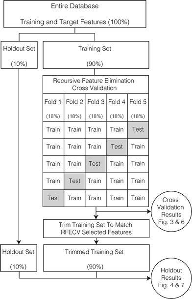
Partitioning the database into training, cross validation, and testing data sets is critical to evaluate the performance of the machine learning effort (n.b., the testing partition is called the ‘holdout’ partition to prevent confusion with cross validation testing). A schematic of the partitioning and model structure is shown in Fig. 2 and supplemented with a textual description.

Fig. 2 Graphical depiction of data partitioning scheme and model structure for the classification and regression problems. The fraction of training and target features employed for each step are shown in parentheses. In the first step, the database is divided into the holdout set (10%) and the training set (90%). No training is performed on the holdout set training features. Instead, the model is trained using the training set and the unimportant features are removed from the database using recursive feature elimination with cross validation (RFECV). The model is retrained on the ‘trimmed’ training set and evaluated using the holdout set.

Overall, 500 model runs were performed. For each model run the following steps were carried out:

1. All usable experiments within the database were randomly assigned to the holdout (10%) or training (90%) data sets. No training was performed on the holdout set.

• The training-holdout split was random for the regression problem.

• The training-holdout split was random for the classification problem, but the ratio of RP shape classes was preserved between datasets. The purpose of this stratified split is to mitigate the influence of class imbalance on the random forest classification,³⁵ which favors hyperexponential RPs (Table 2).

Table 2 Distribution of observations by RP shape within the database. RP shapes that can be modeled using PTMs (HE, EXP) are separated from those that cannot (SIR, IRwD, LD)

Retention profile class	Count
Hyperexponential (HE)	103
Exponential (EXP)	32
Suppressed Inlet Retention (SIR)	30
Increasing retention with Depth (IRwD)	11
Linearly Decreasing (LD)	7

---

2. Recursive feature elimination with 5-fold cross validation (RFECV) was performed using random forests generated from the training set (specifically, from the temporary database formed by four folds in combination). Because there are five cross-validation folds, five RFECV iterations were performed in each model run.

• The cross validation training-testing split was random for the regression problem.

• The cross validation training-testing split was random for the classification problem, but the ratio of RP shape classes was preserved in each cross-validation fold.

• Regression performance was assessed using the MSE; classification performance was assessed using the F1-score;³¹ these metrics are called “cross-validation score” below.

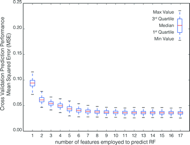
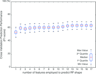
• For each of the five RFECV iterations, the RFECV routine generates 17 random forests (with the feature set size decreasing from 17 to 1) and reports the feature set size corresponding to the highest cross-validation score (i.e., the ‘optimum number of features’).³⁰ If two or more feature set sizes have the same score, the smallest set size is recorded. The optimum number of features indicates the minimum number of features required to maximize the cross-validation score for a particular cross-validation fold.

• Aggregated-cross validation results show model performance as a function of feature set size for all 500 model runs, as shown in Fig. 3 and 6.

Fig. 3 Aggregate model performance in predicting the RF of the cross-validation test fold as a function of the number of features employed to train. Each box plot represents aggregated model scores for five cross-validation iterations for all 500 model runs. This results in 2500 data points for each feature set size.

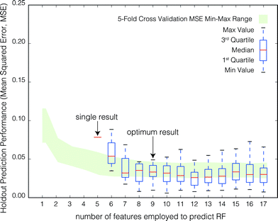Fig. 4 Aggregate model performance in predicting the RF of the holdout set as a function of the number of RFECV-selected features employed to train the model. For each model run, the training database was trimmed to match the feature set selected by RFECV. The model was then re-trained on the trimmed database and the model prediction accuracy (measured by the MSE) was evaluated using the holdout set. For each of the 500 model runs, the prediction MSE and the RFECV-selected feature set size were recorded. Box plots represent the distribution of holdout prediction MSE by feature set size. Note that the trimmed database varies in size and composition due to randomness in the data selection process in RFECV. Feature sets consisting of less than 4 features were never selected by RFECV and only 1 of the 500 RFECV feature sets consisted of only 4 features. The 5-fold cross validation MSE (Fig. 3) min–max range is shown in green to gauge model performance on the holdout set.

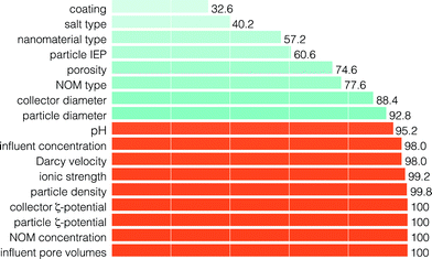Fig. 5 The frequency of features included through RFECV (in percent of number of model runs) for the prediction of the RF. The feature set corresponding to the optimum result, as determined by eqn (1), is presented in orange.

Fig. 6 Aggregate model performance (F1-score) in predicting the RP shape class of the cross-validation test fold as a function of the number of features employed to train. Box plots represent aggregated model scores for five cross-validation iterations for all 500 model runs. This results in 2500 data points for each feature set size.

3. The training set was ‘trimmed’ to the features identified by RFECV (i.e., reduced to the features corresponding to the optimum number of features as it was identified in step 2). A new random forest model was then trained on the trimmed training set and evaluated against the holdout set.

• For each model run, the values of the holdout set training features are used as model inputs and the accuracy of the prediction is evaluated against the holdout set target features.

• Aggregated holdout results, as displayed in Fig. 4 and 7, show the predictive performance as a function of feature set size for all 500 model runs (500 data points in total). From the aggregated results for all model runs, the optimal feature set size (optimum result) was derived by weighting the number of features, the median prediction error, and the variance, i.e., lower model performance with fewer features and lower variance is preferred over a larger feature set with better performance, but higher variance. The optimum feature set size was determined by means of the following performance-variance-feature set trade-off equation:

where n_features is the number of features employed in a given model run, E is the median MSE for the model runs with feature set size n_features, and r_IQ is the interquartile range of the holdout performance for the set of model runs with feature set size n_features.³⁶E is the median MSE for the regression problem and 1 minus the median F1-score for the classification problem.

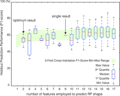Fig. 7 Aggregate model performance to predict the RP shape for the holdout set as a function of the number of RFECV-selected features employed to train the model. For each of 500 model runs, the prediction F1-score and the RFECV-selected feature set size were recorded. Box plots represent the distribution of holdout prediction F1-Scores by feature set size. The 5-fold cross validation F1-Score (Fig. 6) min–max range is shown in green to gauge the performance of holdout set.

It is important to note that all 500 model runs were considered equally important and the random forests trained on the trimmed feature sets given the same weight. Because the training sets from which the random forest models are randomly generated, and thus the optimum feature set identified through RFECV varies between model runs, no “final” model exists.

To identify the most important features, we present a feature ranking in Fig. 5 and 8 that indicates how often a feature occurs in the 500 feature subsets that obtained the optimum score in the RFECV. This allows quantitative assessment of each feature in terms of its influence on the prediction. For example, important features will have an RFECV selection frequency near 100%, as these features are consistently selected. Weaker, but still relevant features will have lower, but non-zero selection frequencies, as these features are selected when stronger features are not present in the currently selected subset. Weak or relatively irrelevant features will have scores close to zero, as they are infrequent among the selected features.³⁰

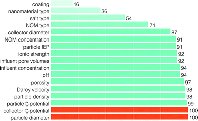Fig. 8 The frequency of features included through RFECV (in percent of number of model runs) for the prediction of RP shape class. The feature set corresponding to the optimum result, as determined by eqn (1), is presented in orange.

3. Results and discussion

3.1. Prediction of the retained fraction (RF)

3.1.1 RF prediction during cross validation. In Fig. 3, the aggregate performance of the model in predicting RF is shown as a function of the number of features employed to train the model during cross validation. Visual inspection indicates that the increase in median cross-validation performance is relatively small (≪0.01 MSE) for greater than 5–6 features.

3.2.1 RF prediction for the holdout set

Fig. 4 shows the aggregate performance of the model in predicting the RF for the holdout set as a function of the number of RFECV-selected features employed to train the model. The best prediction of the RF, or lowest median MSE, was obtained for feature sets consisting of 12 features selected by RFECV (median MSE = 2.61 × 10⁻²; r_IQ = 1.70 × 10⁻²). However, the optimum result, as determined by eqn (1), was obtained for feature sets consisting of 9 features (median MSE = 3.3 × 10⁻²; r_IQ = 1.44 × 10⁻²).

Fig. 5 shows the features according to their frequency of occurrence in all 500 model runs. The nine features corresponding to the optimum result are identified in orange.

In general, RF prediction for the holdout set was better than during cross-validation. This is expected, as the cross validation data sets are smaller than the total training set (72% of the total data set is employed for each cross-validation iteration [4 of 5 folds of the training set]; 90% is employed for each holdout iteration [i.e., the total training set]). Note that there are no holdout scores for 1–4 features. During cross validation the model performance, when the model was trained with less than four features, was always less than that when trained with four or more features. Therefore, the ‘optimum feature set’ determined by RFECV (Section 2.4, Step 2), which is employed as a guide to trim the database to the most suitable set of features, never consists of less than four features.

Several interesting findings are noted. First, our results suggest that the salt type has a relatively low importance in predicting the RF. This seems surprising, particularly as many studies report strong influences of bivalent cations (specifically Ca²⁺) that cannot be accounted for by ionic strength alone (e.g., bridging effects).^4,18,37,38 However, authors often lower the concentration of multivalent cations to be within the same range of influence as monovalent cations (e.g., Chen et al.¹⁸ tests 0.56 mM NaCl against 0.02252 mM CaCl₂). This reduces the ability of the models to ascertain the true influence of salt type on NM transport.

Second, our results suggest that the pH is of greater importance in predicting the RF than the IEP, although both are generally considered relevant for assessing NM stability in suspension.^38,39 This is in line with previous work that qualitatively establishes the importance of pH.^5,17–21 Also, we find that the number of influent pore volumes and the influent concentration are critical to predicting the RF. This is well understood mechanistically, and provides further validation that relevant features are identified.

Third, and most intriguingly, we find that the NM type is relatively unimportant to predict the RF. Several publications indicate that NP fate and behaviour cannot be generalized and that each NP needs to be tested individually.^40,41 However, the machine learning results presented here provide evidence that this may not be the case. The interpretation of this finding is that, within the set of physicochemical features employed here, the behavior of the NMs is nearly entirely captured without needing to consider any NM-specific (i.e., associated with the NM type) interaction.

3.2. Prediction of the retention profile (RP) shape

3.2.1 RP shape prediction during cross validation. The aggregate performance of the model in predicting RP shape as a function of the number of features employed to train the model during cross validation is shown in Fig. 6. Visual inspection indicates that model performance does not strongly improve with increasing number of features.

3.2.2 RP shape prediction for the holdout set. The aggregate performance of the model to predict the RP shape of the experiments in the holdout set as a function of the number of RFECV-selected features employed to train the model is shown in Fig. 7. In general, the prediction of RP shape class is poor. The highest expected F1-score was obtained when 11 features were employed for training (median F1-score = 68%; r_IQ = 0.14%). The optimum result, as determined by eqn (1), was obtained for feature sets consisting of only two features (median F1-Score = 56.3% r_IQ = 0.05%). The highest expected performance of the classifier (F1-score of 68%) only provides an increase of 13% above guessing all RPs are HE (56% of the profiles are HE), and the optimum result (classifiers using two features) provides virtually no predictive improvement. This result was not entirely unexpected, as significant class imbalance is present in the data; that the methodology was tailored to reduce these biases (stratified training-holdout split procedure and RFECV [Section 2.4]) did not really compensate for the limitations of the data set. However, it is also possible that relevant physicochemical features were not included, although we have exhausted the majority of measurable parameters.⁴²

The stability of the feature set selected by RFECV was evaluated by examining feature inclusion frequencies over all 500 model runs (Fig. 8). The poor class prediction, and low improvement in prediction with increasing number of features, make it difficult to extract meaningful results. Some interesting aspects can still be noted. First, similar to predicting the RF, the NM type and salt type were of low importance in predicting the RP shape. Second, the NOM concentration and ionic strength were more important than the NOM type and salt type in predicting the RP shape. The importance of NOM concentration on the RP shape is supported by experimental observations made by Liang et al.²¹ and Chen et al.,⁷ where manipulation of the concentration of surfactant in solution was observed to cause RP shape changes. However, there are too few experiments and too many NOM types to examine to definitively rule out nanomaterial type, salt type, or NOM type as important features. Finally, although the optimum result consists of only two features, 11 features were included in more than 90% of model runs (Fig. 8).

4. Conclusions

In contrast to mechanistic models, which are unable to describe transport (let alone predict it) when non-exponential retention profiles are observed, the applied machine learning regression approach enables prediction of the RF with an MSE < 2.6 × 10⁻². This approach enables quantitative prediction of nanomaterial transport distance independently of a mechanistic understanding of NM behavior. We anticipate that this method could be used to support high-throughput risk screening to identify conditions with high or low vertical mobility of NM in porous media without costly and time-intensive experimental work. Further, we foresee this approach facilitating the development of materials specifically designed to accumulate, or transport, in response to varying physico-chemical conditions.

Mechanistic PTMs are important, but currently not suitable for quantitatively describing and predicting NM transport in porous media. As such, a hybrid mechanistic and machine-learning approach may offer a way to reconcile problems with mechanistic models. As a first step, ranges of physico-chemical conditions may be defined where the current mechanistic models are sufficient. This might be accomplished by a reformulation of the presented multi-class classification problem as a binary problem (exponential vs. non-exponential RPs). For conditions that result in non-exponential RPs, transport equations need to be modified, or alternatively parameterized, using the established method to predict the RF.

Empirical approaches such as the one employed here have limitations, too. For instance, if the data available for the assessment are not representative, the utility of the approach will be low. In particular, we caution extension of the applicability of this work to real soils, as no column transport studies in real soils were employed for this work. Furthermore, for the classification problem serious data limitations currently prevent adequate understanding of how physicochemical conditions influence the shape of the retention profile. The poor performance of the classification predictor is most likely a result of the limited and highly biased data that were available for this work.

In this work we demonstrate that machine learning methods not only add value to the development of mechanistic models through identification of the important features affecting the fate of materials in the environment, but they have the potential to create a new, flexible, and prediction-oriented class of NM transport models. However, for an improved understanding of nanoparticle transport in porous media, several changes in experimental design and data presentation are required. First, and in relation to the physicochemical features identified as important in this work, the existing body of literature must be reviewed to determine what kind of data are already available, what the scope and meaning of these data is, and where exactly the most important data gaps exist. Second, future experimentation must proceed in a manner that fully exploits the information on the physicochemical conditions of column transport experiments, while minimizing cost and time resources.⁴³ On this basis, machine-learning methods can generate more transparent relationships between nanoparticle transport and experimental conditions and, thereby, provide a basis for the development of improved mechanistic models of nanoparticle transport in porous media.

5. Abbreviations

DLVO	Derjaguin, Landau, Verwey and Overbeek
EXP	exponential
HE	hyperexponential
IEP	isoelectric point
IRwD	increasing retention with depth
LD	linearly decreasing
MSE	mean squared error
NM	nanomaterial
NOM/NOL	natural organic matter/natural organic ligands
PTM	particle transport model
SIR	suppressed inlet retention
RF	retained fraction
RFECV	recursive feature elimination with cross validation
RP	retention profile

Acknowledgements

We thank Nicole Sani-Kast for helpful comments.

References

1. J. F. Schijven, S. M. Hassanizadeh and R. H. de Bruin, J. Contam. Hydrol., 2002, 57, 259–279.
2. S. A. Bradford, J. Simunek, M. Bettahar, M. T. van Genuchten and S. R. Yates, Environ. Sci. Technol., 2003, 37, 2242–2250.
3. N. Tufenkji and M. Elimelech, Environ. Sci. Technol., 2005, 39, 3620–3629.
4. I. Chowdhury, Y. Hong, R. J. Honda and S. L. Walker, J. Colloid Interface Sci., 2011, 360, 548–555.
5. L. Cai, M. Tong, H. Ma and H. Kim, Environ. Sci. Technol., 2013, 47, 5703–5710.
6. C. C. Choy, M. Wazne and X. Meng, Chemosphere, 2008, 71, 1794–1801.
7. G. Chen, X. Liu and C. Su, Environ. Sci. Technol., 2012, 46, 7142–7150.
8. E. Goldberg, M. Scheringer, T. D. Bucheli and K. Hungerbühler, Environ. Sci. Technol., 2014, 48, 12732–12741.
9. S. A. Bradford, J. Simunek and S. L. Walker, Water Resour. Res., 2006, 42, 1–12.
10. J. A. Redman, S. L. Walker and M. Elimelech, Environ. Sci. Technol., 2004, 38, 1777–1785.
11. A. R. Petosa, D. P. Jaisi, I. R. Quevedo, M. Elimelech and N. Tufenkji, Environ. Sci. Technol., 2010, 44, 6532–6549.
12. M. Elimelech and C. R. O'Melia, Environ. Sci. Technol., 1990, 24, 1528–1536.
13. M. W. Hahn and C. R. O'Melia, Environ. Sci. Technol., 2004, 38, 210–220.
14. A. Dale, E. A. Casman, G. V. Lowry, J. R. Lead, E. Viparelli and M. A. Baalousha, Environ. Sci. Technol., 2015, 49, 2587–2593.
15. J. M. Gernand and E. A. Casman, IEEE Intelligent Systems, 2014, 29, 84–88.
16. D. Winkler, F. Burden, B. Yan, R. Weissleder, C. Tassa, S. Shaw and V. Epa, SAR QSAR Environ. Res., 2014, 25, 161–172.
17. Y. Wang, Y. Li, J. D. Fortner, J. B. Hughes, L. M. Abriola and K. D. Pennell, Environ. Sci. Technol., 2008, 42, 3588–3594.
18. G. Chen, X. Liu and C. Su, Langmuir, 2011, 27, 5393–5402.
19. X. Liu, G. Chen and C. Su, Environ. Sci. Technol., 2012, 46, 6681–6688.
20. T. Tosco, J. Bosch, R. U. Meckenstock and R. Sethi, Environ. Sci. Technol., 2012, 46, 4008–4015.
21. Y. Liang, S. A. Bradford, J. Šimůnek, H. Vereecken and E. Klumpp, Water Res., 2013, 47, 2572–2582.
22. E. H. Jones and C. Su, Water Res., 2012, 46, 2445–2456.
23. E. Jones and C. Su, J. Hazard. Mater., 2014, 275, 79–88.
24. D. Wang, W. Zhang and D. Zhou, Environ. Sci. Technol., 2013, 47, 5154–5161.
25. D. Wang, S. A. Bradford, R. W. Harvey, X. Hao and D. Zhou, J. Hazard. Mater., 2012, 229, 170–176.
26. D. Kasel, S. A. Bradford, J. Šimůnek, M. Heggen, H. Vereecken and E. Klumpp, Water Res., 2013, 47, 933–944.
27. D. Wang, W. Zhang, X. Hao and D. Zhou, Environ. Sci. Technol., 2013, 47, 821–828.
28. E. Vitorge, S. Szenknect, J. M.-F. Martins, V. Barthès and J.-P. Gaudet, Environ. Pollut., 2014, 184, 613–619.
29. L. Breiman, Mach. Learn., 2001, 45, 5–32.
30. F. Pedregosa, G. Varoquaux, A. Gramfort, V. Michel, B. Thirion, O. Grisel, M. Blondel, P. Prettenhofer, R. Weiss, V. Dubourg, J. Vanderplas, A. Passos, D. Cournapeau, M. Brucher, M. Perrot and E. Duchesnay, J. Mach. Learn. Res., 2011, 12, 2825–2830.
31. C. van Rijsbergen, Information Retrieval, Butterworths, 1979.
32. K. K. Nicodemus, J. D. Malley, C. Strobl and A. Ziegler, BMC Bioinf., 2010, 11, 110.
33. G. Louppe, L. Wehenkel, A. Sutera and P. Geurts, in Advances in Neural Information Processing Systems 26, ed. C. Burges, L. Bottou, M. Welling, Z. Ghahramani and K. Weinberger, Curran Associates, Inc., 2013, pp. 431–439.
34. C. Strobl, A.-L. Boulesteix, A. Zeileis and T. Hothorn, BMC Bioinf., 2007, 8, 25.
35. S. Dudoit and J. Fridlyand, Bioinformatics, 2003, 19, 1090–1099.
36. R. E. Walpole, R. H. Myers, S. L. Myers and K. Ye, Probability and statistics for engineers and scientists, Macmillan New York, 1993, vol. 5.
37. T. Ben-Moshe, I. Dror and B. Berkowitz, Chemosphere, 2010, 81, 387–393.
38. R. A. French, A. R. Jacobson, B. Kim, S. L. Isley, R. L. Penn and P. C. Baveye, Environ. Sci. Technol., 2009, 43, 1354–1359.
39. K. A. Dunphy Guzman, M. P. Finnegan and J. F. Banfield, Environ. Sci. Technol., 2006, 40, 7688–7693.
40. S. J. Klaine, P. J. Alvarez, G. E. Batley, T. F. Fernandes, R. D. Handy, D. Y. Lyon, S. Mahendra, M. J. McLaughlin and J. R. Lead, Environ. Toxicol. Chem., 2008, 27, 1825–1851.
41. J. S. Tsuji, A. D. Maynard, P. C. Howard, J. T. James, C.-W. Lam, D. B. Warheit and A. B. Santamaria, Toxicol. Sci., 2006, 89, 42–50.
42. S. B. Kotsiantis, I. Zaharakis and P. Pintelas, Supervised machine learning: A review of classification techniques, 2007.
43. T. Guest and A. Curtis, J. Geophys. Res.: Solid Earth, 2009, 114, B04307.

---

Footnote

† Electronic supplementary information (ESI) available. See DOI: 10.1039/c5en00050e

---