
 Open Access Article
 This Open Access Article is licensed under a
 Creative Commons Attribution 3.0 Unported Licence
Agricultural livelihoods in coastal Bangladesh under climate and environmental change – a model framework†
Attila N.
Lázár
*a,
Derek
Clarke
a,
Helen
Adams
b,
Abdur Razzaque
Akanda
c,
Sylvia
Szabo
a,
Robert J.
Nicholls
a,
Zoe
Matthews
a,
Dilruba
Begum
d,
Abul Fazal M.
Saleh
e,
Md. Anwarul
Abedin
f,
Andres
Payo
a,
Peter Kim
Streatfield
d,
Craig
Hutton
a,
M. Shahjahan
Mondal
e and
Abu Zofar Md.
Moslehuddin
f
aUniversity of Southampton, University Road, Southampton, Hampshire SO17 1BJ, UK. E-mail: a.lazar@soton.ac.uk
bCollege of Life and Environmental Sciences, University of Exeter, Prince of Wales Road, Exeter, Devon EX4 4SB, UK
cBangladesh Agriculture Research Institute, Joydebpur, Gazipur-1701, Bangladesh
dInternational Centre for Diarrhoeal Disease Research, Bangladesh, Dhaka-1000, Bangladesh
eBangladesh University of Engineering & Technology, Dhaka-1000, Bangladesh
fBangladesh Agriculture University, Mymensingh, Bangladesh
First published on 22nd May 2015
Abstract
Coastal Bangladesh experiences significant poverty and hazards today and is highly vulnerable to climate and environmental change over the coming decades. Coastal stakeholders are demanding information to assist in the decision making processes, including simulation models to explore how different interventions, under different plausible future socio-economic and environmental scenarios, could alleviate environmental risks and promote development. Many existing simulation models neglect the complex interdependencies between the socio-economic and environmental system of coastal Bangladesh. Here an integrated approach has been proposed to develop a simulation model to support agriculture and poverty-based analysis and decision-making in coastal Bangladesh. In particular, we show how a simulation model of farmer's livelihoods at the household level can be achieved. An extended version of the FAO's CROPWAT agriculture model has been integrated with a downscaled regional demography model to simulate net agriculture profit. This is used together with a household income–expenses balance and a loans logical tree to simulate the evolution of food security indicators and poverty levels. Modelling identifies salinity and temperature stress as limiting factors to crop productivity and fertilisation due to atmospheric carbon dioxide concentrations as a reinforcing factor. The crop simulation results compare well with expected outcomes but also reveal some unexpected behaviours. For example, under current model assumptions, temperature is more important than salinity for crop production. The agriculture-based livelihood and poverty simulations highlight the critical significance of debt through informal and formal loans set at such levels as to persistently undermine the well-being of agriculture-dependent households. Simulations also indicate that progressive approaches to agriculture (i.e. diversification) might not provide the clear economic benefit from the perspective of pricing due to greater susceptibility to climate vagaries. The livelihood and poverty results highlight the importance of the holistic consideration of the human–nature system and the careful selection of poverty indicators. Although the simulation model at this stage contains the minimum elements required to simulate the complexity of farmer livelihood interactions in coastal Bangladesh, the crop and socio-economic findings compare well with expected behaviours. The presented integrated model is the first step to develop a holistic, transferable analytic method and tool for coastal Bangladesh.
Environmental impactClimate- and human-induced environmental and livelihood changes are growing concerns around the world's coastlines, especially populous deltas. This paper proposes an integrated model of the human–natural farming system that supports 40 million people in coastal Bangladesh alone. It proposes appropriate methods and scales for crop simulation, demographic projection and livelihood analysis that are meaningful in terms of both scientific and stakeholder needs. This paper provides insights not only into the relative importance of soil salinity and air temperature, but also the relationship between crop yield, livelihood and poverty. This integrated model is the first step towards an operational integrated assessment framework for coastal Bangladesh that is also transferable to other agricultural deltas. |
Introduction
Bangladesh has long been considered to be one of the most vulnerable countries in the world given human-induced climate change and subsequent sea-level rise.1 It is estimated to be the third most vulnerable country in terms of population exposed to sea level rise.2 Coastal Bangladesh is also a hub of hydro-meteorological disasters including cyclones, tidal surges, floods, drought, saline water intrusion, waterlogging, and land subsidence. This has a direct bearing on livelihoods as agriculture provides employment for over 60 percent of the population in Bangladesh3 and it is a key economic activity for the 40 million inhabitants in the coastal zone.4 Rain-fed rice is the dominant crop grown in the monsoon period, and irrigation is necessary in the dry season to grow rice, pulses, oil seeds and vegetables. The agricultural system is heavily dependent on environmental factors such as the timing, intensity and distribution of the monsoon, soil salinity and the availability of freshwater for irrigation. Anticipated climate change effects suggest that total rainfall in the coastal area is unlikely to decrease in the future.5,6 Higher temperatures, changes in monsoon timing and predictability,7 sea-level rise and land subsidence driven by natural and human activities8,9 will make farming less secure as a livelihood unless there is improved farm management.Bangladesh is not only vulnerable to the impacts of climate change. It also has a growing population (139 million in 2011) with one of the highest population densities in the world (950 individual km−2), of which a large proportion live in poverty (∼43%), and has real barriers to overcome in terms of continuing to feed its population. Rural livelihoods in Bangladesh are complex, showing migratory interactions with urban areas10 and livelihood diversification into off-farm incomes. Indeed only around half of the population has access to land, and the land is concentrated in the hands of a small proportion of people. Powerful landlords employ the landless as agriculture labourers. Thus, to understand the effect of the changing agriculture productivity on people, any analysis should investigate not only the impact of environmental change on productivity, but also the access to land, the ability of households to turn different farming practices into income, and the distribution of profits from the land.
Bangladesh's ambition is to become a middle income economy, reducing poverty substantially, and promoting and sustaining health and nutrition for 85 percent of its population by 2021.11 To achieve this ambitious plan, integrated governance is required that considers climatic, environmental and socio-economic changes. This must be underpinned by studies that include macro- and micro-scale processes and the interlinked human–nature system. Numerical models are capable of representing complex systems and calculating uncertainties around the most likely results. Many agricultural, economic and social science models are available in the published literature with varying complexity. The majority of these models focus on a single discipline and only a minority of these numerical models attempt to link natural and social sciences together. These integrative approaches can be classified as GIS-based static models,12,13 system dynamics models,14,15 agent-based models16,17 or Bayesian network models.18,19 However, according to the knowledge of the authors, no model in the published literature attempts to capture both macro- and micro-scale environmental and climate processes and link these to the welfare of households or individuals at the local scale.
The aim of this paper is to develop a medium-complexity model framework and to carry out a preliminary investigation of (i) the effect of climate and environmental change on crop productivity, (ii) the cumulative consequences of crop productivity, demographical changes and market conditions on the well-being and poverty levels of coastal Bangladesh, and (iii) the uncertainties associated with the integrated framework. This approach is accomplished by using an innovative integrated model framework that couples demographic, agriculture and a newly-developed household livelihood model. This paper describes the study area in Section 2, introduces the applied methodologies in Section 3, and shows some preliminary results in Section 4. These results are discussed with reference to the literature, and the advantages and disadvantages of the integrated model are also deliberated in Section 4. Further application and development of the integrated model are outlined in the conclusion.
Study area overview
This study is based on the south-western coastal zone of Bangladesh, where there is a tidal influence. The study area is 18![[thin space (1/6-em)]](https://www.rsc.org/images/entities/char_2009.gif) 850 km2 (Fig. 1), having about 14 million inhabitants with an average population density of 750 people km−2. Administratively the area comprises three districts from the Khulna Division (Satkhira, Khulna and Bagerhat), and all six districts of the Barisal Division of Bangladesh. The nine districts are made up from 70 upazilas (i.e. sub-district administrative units, average size: 264 km2) and 653 unions (i.e. the smallest planning unit in Bangladesh incorporating a few villages, average size: 28 km2, average population: 21800) within the study area.
850 km2 (Fig. 1), having about 14 million inhabitants with an average population density of 750 people km−2. Administratively the area comprises three districts from the Khulna Division (Satkhira, Khulna and Bagerhat), and all six districts of the Barisal Division of Bangladesh. The nine districts are made up from 70 upazilas (i.e. sub-district administrative units, average size: 264 km2) and 653 unions (i.e. the smallest planning unit in Bangladesh incorporating a few villages, average size: 28 km2, average population: 21800) within the study area.
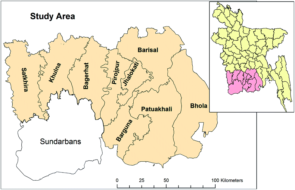 | ||
| Fig. 1 Study area. | ||
This area is extremely low-lying: the land elevation above sea level ranges from one to three metres, but most of the study area is enclosed by embankments to reclaim land (i.e. poldered). The tidal range in this part of Bangladesh varies between 0.5 and 4.5 metres. The land cover in 2010 was dominated by agriculture (45%), followed by natural vegetation (12%), aquaculture (11%), water (8%) and wetland (8%). This deltaic region provides a range of important ecosystem services which make it highly suitable for agriculture which provides livelihoods for the majority of the coastal population. The delta plain of the Ganges–Brahmaputra–Meghna river system supports numerous ecosystem services and livelihoods. About 85 percent of the people of the coastal zone depend on agriculture. As a result of the high population density, over 50 percent of the households are practically landless having less than 0.2 hectares of land. Fishing, crop agriculture, shrimp farming, salt farming, and tourism are the area's main economic activities.20
Bangladesh attained self-sufficiency in food production in 1999–2000 with a gross production of rice and wheat of 24.9 million metric tons which marginally met the country's requirement of 21.4 million metric tons for the population.21 Currently annual rice production alone is 34 million metric tons against a total food grain (rice, wheat and maize) requirement of 30 million metric tons.22 In the case of wheat, the current annual production is sufficient for 33 percent of the population and the rest is imported.
There are three distinct seasons in agriculture: Rabi season (November–March; cool, dry winter), Kharif-1 season (March–June; hot humid summer) and Kharif-2 season (June–November; monsoon). In the 1990s, farms practiced mono cropping (i.e. having only one season crop), but more recently crops have been cultivated in two and three cycles per year. Multi-cropping has become more common because of a higher awareness of alternative crops due to agricultural extension services and non-governmental organisation (NGO) interventions. Additionally, a higher availability of irrigation water, through the installation of diesel-driven tube-wells funded by NGO loans has enabled the capital investment required for high yielding varieties (HYVs).23 The traditional crop is rice (Boro, Aus, Aman), but cash-crop production is increasing and includes crops such as wheat, chilli, potato, mustard, tomato and grass pea. Furthermore, as a result of agricultural research and development projects, the traditional local varieties of crops are almost completely replaced by more resilient hybrid and HYVs.
The highest average maximum temperature in the study area is 33 °C and above during March and May, and the lowest average minimum temperature is about 15 °C in December and January. The south-western region of Bangladesh receives an average rainfall of about 1730 mm per annum, of which about 78 percent falls within the 4 months of monsoon.24 Monsoon rains are important for both providing soil moisture and irrigation water, and flushing the salinity from the soils (Fig. 2). However, soil salinity is more spatially variable due to localised environmental processes and management practices (e.g. irrigation, polderisation, etc.).
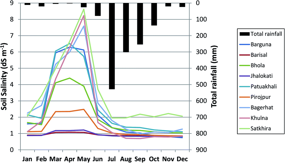 | ||
| Fig. 2 Seasonality of soil salinity (district average) and total rainfall (study area). Data shown for 2009 as an illustration (see Section 3a for more details). | ||
Bangladesh has undergone a considerable demographic change over the last 30 years: rapid fertility decline has been coupled with considerable decrease in mortality. For example, the total fertility rate (TFR) declined (1993–2011) from 3.1 to 1.9 and from 3.5 to 2.3 in the Khulna and Barisal division, respectively.25,26 These changes have been initiated by the comprehensive family planning program and improved access to sexual and reproductive health services. There has also been a considerable increase in out-migration from the study area which has contributed to an overall population decline in some districts. These demographic changes have been coupled by uneven urban growth. While in some districts, including Barisal, the proportion of urban population continues to increase, in other districts, such as Khulna, there is a reverse trend. As a result of the economic improvements and other governance interventions, there has been a significant reduction in the national poverty level (from 70 to 43 percent in between 1992 and 2010, US$1.25 per day poverty indicator).27 However, despite this decreasing trend and fertile land, poverty levels are still high in the coastal region and it is difficult to anticipate that the same poverty reduction trends can be sustained under climate and environmental change.28
Food insecurity closely mirrors the poverty levels: food expenditure is nearly 60 percent of the total expenditure of an average rural household. Rice is the most important staple food, providing 71 percent of the calorific intake.29 Thus, food insecurity forces people to diversify their livelihoods and possibly to migrate internally or internationally.30 Finally, frequent environmental disasters (river flooding and cyclones) with three to five years return periods endanger lives and cause large (crop and asset) losses and can produce degraded land (due to inundation and salinization) that makes the poverty reduction efforts more difficult.
The proposed integrated methodology
A model has been developed to simulate the livelihood and poverty changes of farmers in coastal Bangladesh under climate and environmental change. To do this, crop productivity is linked with demographic changes, market price changes and other socio-economic indicators (e.g. household expenditure) as illustrated in Fig. 3. Elements of this coupled model work at different spatial and temporal scales as shown in Fig. 3 are described in detail below. This was needed to balance out the spatial and temporal scale of observations, meaningful scientific methods, computational requirement and yet useful results for decision making.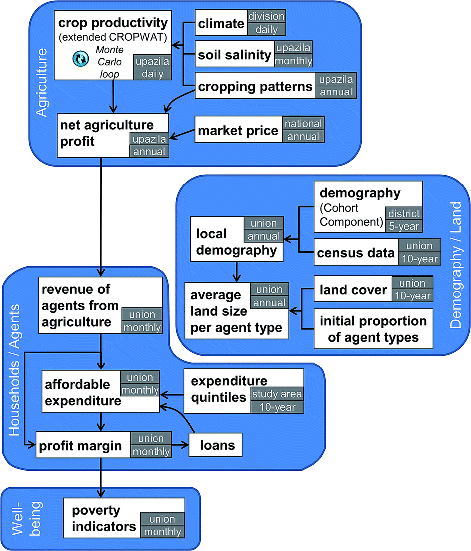 | ||
| Fig. 3 The proposed integrated model structure. The spatial and temporal scales of the model elements are shown in the grey boxes. | ||
Crop productivity is estimated using the extended CROPWAT model calculated separately for all 70 upazilas (sub-districts). This spatial scale is a compromise between data limitation (observed yields, cropping patterns and soil characteristics), computational time and the ability to show spatial variation in results. The net profit of the produce obtained from agriculture is estimated from market price time series. Demographic projections are carried out at the district level and at a five-year calculation time step. The annual population size is obtained from a combination of the annual (linear) interpolation of the district level results and from Census data that describes the population distribution within each district. Population change and the total agricultural land are important determinants of the available land for each household of the simulated farmer agent types (large land owners, small land owners, sharecroppers and landless labourers) within each union, because population increase can lead to land fragmentation through inheritance. The household economy is modelled by comparing the totals of farmers' revenue and savings (cash or assets) with observed monthly expenditure levels and estimates the affordable expenditure level of the simulated agent type for each month. If a household cannot meet its minimum requirement, they are assumed to obtain a loan to cover shortfalls. Household economic calculations are done at the union-level each month and for each farmer type. Total expenditure is an indicator of wealth and here it is also used as indication for the typical diet of the household. This link is used to calculate food security indicators such as the calorie intake and hunger periods. The individual model elements are described in the following sections in more detail.
The union scale (28 km2 on average) was decided to be the most appropriate spatial scale for decision makers and thus for presenting the results, because (i) unions are the smallest planning units in Bangladesh, (ii) unions allow fine spatial variations of environmental factors and land use changes to be captured, and (iii) well-being results are still useful without becoming computationally very expensive. The results are presented at a monthly timestep to capture the seasonality of the environment-based livelihoods.
(a) Climate data and soil salinity data
Long term records of rainfall and potential evapotranspiration were used to determine the timing of the monsoon rains and the volumes of water needed for irrigation. Average climate data were derived for the recent past (1990 to present) and compared with the FAO CLIMWAT database.24 Future climate projections (rainfall, temperature) for 2015–2050 were obtained by downscaling a regional climate model (RCM) developed by the UK Met Office.31 This is an atmosphere-only model, driven by boundary conditions from the HadCM3 model with a resolution of 25 km. The SRES A1B annual atmospheric CO2 concentration32 was used to estimate the atmospheric fertilisation of the crops.Due to the sparse soil salinity observations, homogeneous soil salinity time series were generated for the 1990–2009 period by combining the seasonality of observed river salinity33 with observed peak soil salinity.34 For the 2010–2050 period, the observed historical trend in soil salinity simply continued.
(b) Extended CROPWAT model
This paper uses an extended version of the FAO's CROPWAT 4.3 model.35 The equations were re-coded in Matlab based on the original code of Clarke et al.35 to create a fully-coupled integrated model. In addition, the model was extended to include water and salinity stress36 (pp. 176–177), atmospheric fertilisation by carbon dioxide37 (pp. 86–87) and temperature stress. The temperature stress calculation assumes an optimum temperature range (Topt1–Topt2), where growth is not limited by temperature, and beyond this range, growth limitation linearly increases until growth stops at the absolute limits (Tmin, Tmax) (Fig. 4). The calculation of the actual yield is followed by the FAO56 methodology36 by assuming an equal weight of water, salinity, temperature and atmospheric fertilisation limitations in the actual evaporation calculation. For further details, please read ESI document S1.†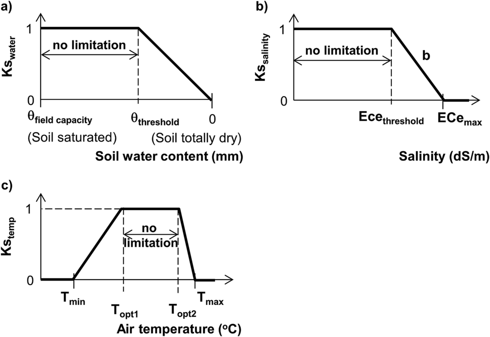 | ||
| Fig. 4 Generic limitation curves: (a) water stress, (b) salinity stress and (c) temperature stress. | ||
A local sensitivity analysis was conducted on the extended CROPWAT model to identify the most important model parameters (ESI document S2†). The aim of the sensitivity analysis was to build an automated uncertainty analysis into the integrated model: varying the most important CROPWAT parameters (±1 std. dev. of the calibrated parameter value) and calculating uncertainty bands of the crop simulations that can be passed on to the subsequent calculations of the integrated model. The calibration of the extended CROPWAT model used a parameter optimisation routine. The optimiser was searching the parameter space to find the local minima of Root Mean Square Error goodness-of-fit coefficient (ESI document S3†).
(c) Cropping patterns
Two important cropping patterns were selected for investigation of the model: a ‘traditional’, and a ‘progressive’ cropping pattern, both of which were observed in the study area in both 1990 and 2010. In the 1990s, mainly local crop varieties were grown, whereas in 2010, the crop production shifted towards high yielding and more resilient varieties as well as an increase in diversity of crop types (Table 1). This is suggested to be due to the dissemination of modern technologies and knowledge through various stakeholders' viz. governmental organization, NGOs and donor agencies. In this study, it is assumed that 50 percent of the farmers continue traditional practice and 50 percent of the farmers adopt a cash-crop cultivation practice. The baseline simulation uses 2010 cropping patterns and the present crop properties.| Type | Time period | Rabi season | Kharif-1 season | Kharif-2 season |
|---|---|---|---|---|
| a Note: HYV – high yielding variety. | ||||
| Traditional cropping pattern | 1990–2000 | Boro rice (HYV) | Fallow | Transplanted Aman rice (local) |
| 2000–2050 | Boro rice (HYV) | Fallow | Transplanted Aman rice (HYV) | |
| Progressive cropping pattern | 1990–2000 | Potato (HYV), grass pea (HYV), chilli (local) | Transplanted Aus rice (local) | Transplanted Aman rice (local) |
| 2000–2050 | Potato (HYV), wheat (HYV), chilli (hybrid) | Transplanted Aus rice (HYV) | Transplanted Aman rice (HYV) | |
(d) Demographic projections and assumptions
The integrated model uses the observed population changes for the historical period, and uses the Cohort Component population projection method to estimate the population changes in the future. This method uses observed data, trends and expert judgments of future changes. A constant scenario for population projections is assumed, where the population change is expected to occur based on a continuation of the current rates of fertility, mortality and migration into the future. Whenever available, district level data are used, primarily from the most recent and historical censuses, Demographic and Health Surveys, the 2010 report on the Sample Vital Registration System38 and statistics developed by the UN Population Division.39In our study area total fertility rates (TFRs) vary between 1.56 and 2.16. For the purpose of the integrated model these district level TFRs are assumed to remain constant over the simulation time period (2011 to 2050). Based on the mortality data from the most recent population census,40 the estimated current life expectancy of males in the study area varies from 71 years for the Khulna division to 68 years in the Barisal division. For females, life expectancy at birth is 73 years in the Khulna division and 70 years in the Barisal division. The model assumes that current levels of life expectancy remain the same until 2050 for both sexes in all districts. Finally, migration, which is often the most difficult population component to model due to its unpredictability, is based on the past trends. Since in 2011 out-migration was considerably higher than in 2001, the future trend is based on the intercensal average.
(e) Household livelihood model
The household livelihood model is based on an income–expenditure balance calculation. It considers (i) the income generated from the crop yield based on the harvest time market prices, (ii) the generalised costs required to run households and (iii) the net profit calculated as the difference between income and costs. Several household-level economic indicators are computed during the model run including revenue, net earnings, loan need and profit margin. For the purposes of this paper, the model only addresses income gained from agriculture. Based on the ESPA Deltas (Summer 2014) Household Survey dataset, only 24 percent of households rely exclusively on agriculture or agriculture labour, and the majority of households have multiple income sources. Therefore, the model does not represent the full household income, but the processes surrounding generating the wellbeing from agriculture.Market prices (harvest time crop and agriculture input prices) were collated from the Bangladesh Bureau of Statistics yearbooks.3,41 Market prices were kept constant in the future at the 2013 level because of the extreme difficulty to predict how Bangladeshi market conditions would change under climate change, macro-economic changes, changes in demand triggered by population growth and technological advancement. This permits us to keep the model assumptions simple, and permits the examination of future livelihood changes against the present economic situation.42
The total household costs (excluding agriculture expenses) in Bangladeshi Taka (BDT) and calorie intake used in this paper are calculated for the study area from the Household Income and Expenditure Survey datasets (Table 2). It is assumed that wealthier households have a different expenditure-level and diet from poorer households. These ‘wealth’ quintiles were approximated by normalising the total household expenditure by the household size. When the wealth-quintiles were assigned to each household, the mean of the quintiles was calculated for total household expenditure and calorie intake per capita per day. These values were inter- and extrapolated to populate the model with monthly cost estimates for the 1981–2013 period. As with the other economic input variables, the 2013 total expenditure and calorie intake levels are used in consecutive years (2014–2050). During the model run, for each month and for each agent-type, the most appropriate (i.e. affordable) household expenditure level is selected by comparing their actual revenue, assumed savings (i.e. cash savings or assets) and expected costs.
| ‘Wealth-level’ | 1991 | 1995 | 2010 | |
|---|---|---|---|---|
| Total expenditure (BDT per household per month) | 1 (poorest) | 1617 | 2021 | 4315 |
| 2 (poor) | 2176 | 2592 | 6240 | |
| 3 (medium) | 2519 | 3447 | 7654 | |
| 4 (rich) | 3290 | 4558 | 9860 | |
| 5 (richest) | 5359 | 8194 | 17281 |
|
| Calorie intake (kcal per capita per day) | 1 (poorest) | 1588 | 1621 | 1599 |
| 2 (poor) | 2008 | 2028 | 2035 | |
| 3 (medium) | 2369 | 2323 | 2313 | |
| 4 (rich) | 2712 | 2523 | 2643 | |
| 5 (richest) | 3031 | 2935 | 3205 |
There are numerous (official and informal) loan types in Bangladesh. This paper considers two types of loan. One is an official loan from the Bangladesh Rural Development Board (BRDB). This loan type is available for agriculture production and to diversify agriculture. The amount of loan is generally 10–35 thousand BDT (22500 BDT in the model, or approximately US$300) with an annual service charge of 11 percent. The return period is 12 months with a weekly re-payment. The annual interest rate of the BRDB loan (i.e. service charge) is one of the lowest currently available on the market, thus providing a ‘best-world’ scenario in the business as usual model runs. The other loan type is an informal (high interest) loan from a private money lender with a 120 percent annual interest rate and a 12 month return period.
The model assumes that if the household expenditure is higher than the revenues plus savings in a particular month, the household automatically applies for the BRDB loan. If this is still not sufficient, the household also gets the informal loan from the private money lender. The number of loans is continuously updated in the model for each union and agent type. The model simplifies reality by assuming that the household meets all requirements (certain amount of collateral, a certain level of income, etc.) and the loan for agriculture is granted instantly (i.e. no waiting time). Conditions for loans can be easily incorporated into future versions of the model, when the details become available. In reality, the BRDB loan can only be used for agriculture, but the model assumes that similar loans exist for other non-production purposes in Bangladesh (wedding, medical treatment) and considers the BRDB loan to be available for any purposes.
This paper focuses on agriculture related livelihoods and more specifically on four different actors: Large Land Owners (LLO, >2 ha land), Small Land Owners (SLO, ∼1 ha land), Sharecroppers (SC – who rent ∼1 ha land to cultivate) and Landless Labourers (LL, ∼0.01 ha land). The proportion of these simulated agents was kept constant in the current version of the model and their ratios were calculated from the ESPA Deltas (Summer 2014) Household Survey dataset (LLO: 3.7%, SLO: 20%, SC: 12.7%, LL: 16.1% of all households). Although the proportion of these agents is fixed during all the simulation years, the associated land size of these agents changes in accordance with the population change. This is because as population increases, the land ownership of the land is split and thus land fragmentation occurs and vice versa. An increase in population also means that the labour force increases thus the surplus labour force has to do off-farm work in the locality or outside the area. An increase in labour force would mean that the wages of the labourers drop, but this socio-economic effect is not simulated in this integrated model. However, the model does include intra-household dynamics, where households send more members out to work, as income falls and their daily expenses are needed to be met. Thus, the integrated model allows the simulated SLO, LL and SC agents to decide how many of their household members have to do labour work to support their living. The number of household members in the simulation doing labour work cannot be larger than the dependency ratio of the household (i.e. young children and elderly cannot work, but others might if necessary to meet the household expenses). Large Land Owners are assumed that they do not do labour work. Rather, they hire labourers to cultivate their fields. Although the model may not represent the rural dynamics in its full complexity, the basic household dynamics are aimed to be captured with this relatively simple livelihood model.
(f) Poverty indicators
Poverty can be measured in different ways. The most widely used indicators relate to the monetary dimensions of well-being (i.e. income and consumption), but other indicators also exist covering the non-monetary dimensions of poverty (health, education, assets, etc.). This paper uses two indicators, one measuring monetary poverty, and the other is a health related, food security indicator. The US$1.25 per person per day poverty indicator is a widely used measure of poverty based on incomes or consumption levels. It compares the per capita per day income or consumption with the country-specific, purchase power parity adjusted US$1.25 threshold value. If the value is below the threshold, the person in question is in monetary poverty. In our paper, income-based poverty is calculated by only considering the farm-related incomes. As a result, the model provides a functional indicator of whether farming by itself is a viable livelihood in coastal Bangladesh.The food insecurity indicator is the calorie intake-based (kcal per capita per day) hunger period length (i.e. the number of months in a year, when the calorie intake is less than 1805 kcal per capita per day). The 2122 kcal per capita per day had been used as a food poverty threshold for Bangladesh.43 The average calorie intake for each wealth quintile was calculated from the HIES datasets (Table 2). By using the affordable expenditure as a proxy, the model is capable of approximating an assumed monthly average calorie intake for each household type (spatially, temporally and for each agent-type separately). If the calorie intake is known, the hunger periods of the households can be easily calculated.
Results and discussion
(a) Crop model sensitivity and uncertainty
Crop simulations are most sensitive to 5 out of 23 parameters. Fig. 5 shows a tornado plot with the sensitivity of the most important parameters. The sensitivity of the parameters changes with crops and season. Overall, the model outputs are the most sensitive to five crop parameters: Ky (yield response factor), the optimum temperatures (Topt1 and Topt2), Kc,mid (crop coefficient – middle growth period) and Ece,b (yield reduction per increase of salinity). During the integrated model runs, these five crop parameters are varied automatically 21 times to estimate the parameter uncertainties of calculated crop yield results. The yield results of these multiple model runs are summarised by calculating the mean, minimum and maximum values, and these are passed on to the livelihood calculation sub-routine.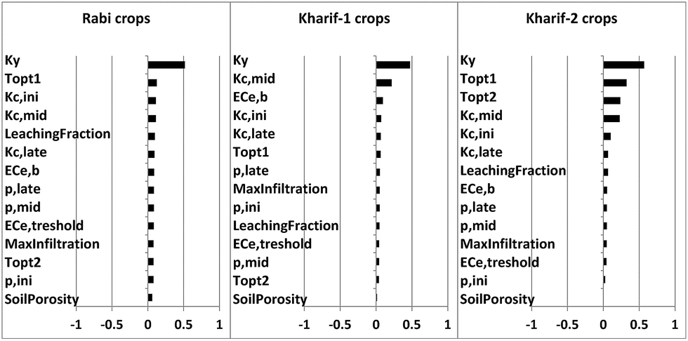 | ||
| Fig. 5 Seasonal sensitivity of CROPWAT parameters. | ||
Two examples for the 21 ensemble members of the CROPWAT uncertainty analysis are shown in Fig. 6. All crops have similar results to Fig. 6a. As a result of the uncertainty calculation method (±1 std. dev.), the ensemble members are clustered around the calibrated value and upper and lower lines, primarily defined by the Ky (yield response factor) value. The distance between the three clusters is different for each crop, and in each time period (1990s, 2000s, future). However, this is not always the case. In the case of Boro rice, the ensemble member clusters lose their coherence and spread out to show a more homogenous pattern in the case of 26 percent of the upazilas indicating that other crop parameters gained greater importance. The mean value of the 21 ensemble members is always very close to the calibrated parameter set. The width of the uncertainty band roughly remains the same over time, because only the soil moisture deficit model variable is dependent on previous years, and it does not accumulate over time. The soil dries up during each Rabi season, and thus the annual model runs are almost independent from each other. However, due to climatic changes, this is not a uniform behaviour: uncertainty of Boro rice increases with time in some upazilas, potato has larger uncertainties in certain years, uncertainty continuously decreases with time for wheat, and uncertainty slightly decreases for Aus and Aman rice. Based on these plots, the future suitability and associated risks of each crop can be assessed, if needed.
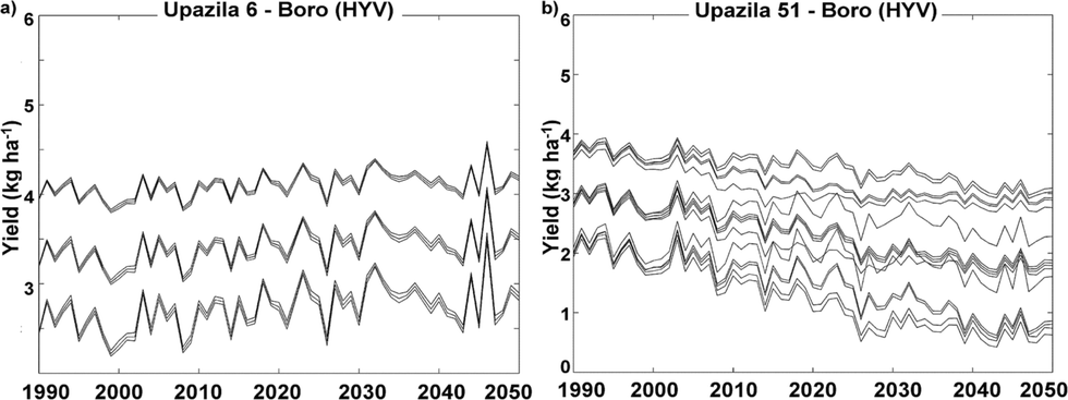 | ||
| Fig. 6 An example for the CROPWAT yield result ensemble members. | ||
(b) Causes of and changes in crop productivity
The integrated model considers the factors affecting crop yield: climate (rainfall, temperature, potential evaporation), environmental (salinity, water availability) and management (irrigation). Crop productivity (i.e. simulated farmers' yield) is found to gently increase over time in the simulations. This is partially due to the fact that local crop varieties have been replaced by hybrid and high yielding varieties, partially due to climatic changes. The relative importance of the climatic factors (i.e. the ‘Ks’ CROPWAT coefficients) is shown in Table 3. Water availability does not significantly affect crop productivity; it only reduces the potential yield by only about 10%. The high water availability coefficient (Kswater) is not surprising, because the Rabi crops are irrigated and the Kharif-2 crops are supported by monsoon.| Traditional farming | Progressive farming | |||||
|---|---|---|---|---|---|---|
| 1990s | 2000s | Future | 1990s | 2000s | Future | |
| KsWater | 0.86 | 0.89 | 0.86 | 0.88 | 0.89 | 0.89 |
| KsSalinity | 0.91 | 0.91 | 0.90 | 0.93 | 0.93 | 0.93 |
| KsTemperature | 0.59 | 0.48 | 0.50 | 0.52 | 0.51 | 0.51 |
| KsCO2 | 0.92 | 0.98 | 1.11 | 0.92 | 0.98 | 1.11 |
Soil salinity, for the assumed cropping patterns, has only a minor influence on the simulated crop yields (10 percent reductions on average). This unexpected low influence of salinity on crop productivity can be explained by overlaying a schematic of the crop calendar with the average annual soil salinity pattern (Fig. 7). It is clear that the highest salinity levels mainly affect the Boro rice development, and only affect the last few weeks of the vegetable growing period. The initial stage of the Aus rice is also affected by salinity. Mondal et al.,44 found that rice is more susceptible to high salinity levels during its initial stages and if salinity increases gradually over its growth period, the yield can be similar to non-saline conditions. Thus, salinity, especially when good quality irrigation water is applied during the dry season, only affects a limited number of crops.
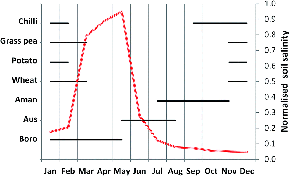 | ||
| Fig. 7 Salinity (red line) only affects the growth period (black horizontal lines) of a few crops. | ||
Temperature has an important effect on the simulated crop yield (KsTemperature), by reducing the simulated yield by about 50 percent on average. Temperature limitation is not observed at present on these crops, but it might occur under future climate change, especially for potato and chilli that have narrower ranges of temperature tolerance. It was concluded that the model parameter optimisation may have compensated for the known uncertainties (e.g. the observed farmers' yield, soil salinity timeseries, etc. – see ESI document S3†) by increasing the temperature limitation of certain crops. This is clearly a limitation of the current version of the integrated model, but this will be amended when both a river and a groundwater salinity model will be fully coupled with a soil salinity model and with the CROPWAT model.
Finally, the atmospheric carbon dioxide (KsCO2) has an important effect on the simulated crop productivities. In the near future, the atmospheric CO2 concentration will reach a level, when the productivity will be enhanced by more than 10 percent. Therefore, if nothing else changes, the same crop can produce more. However, this does not mean that food security can be provided by higher yields. A reanalysis study of existing literature data45 shows that elevated CO2 concentrations boost crop productivity, but the nutrition content of the same crop might be decreased by 10–20 percent. Thus, poorer households might experience negative health effects even though the amount of consumed food is satisfactory.
(c) Environmental and ecological implications of farming
This paper does not aim to assess the environmental consequences of agriculture management, but it is worth briefly mentioning two issues. Increasing atmospheric CO2 concentrations have a positive impact on crop productivity through enhanced atmospheric fertilisation. At the same time, agriculture (mainly fertiliser use and livestock production) is the third largest emission source of greenhouse gases in the world after power/heat generation and transport, and Bangladesh is the 14th largest agriculture-related CO2 emitter (CO2 equivalent of total agriculture emission, 1990–2012 average).46 Based on the current practice in coastal Bangladesh, grass pea requires the least amount of various fertilisers (37 kg ha−1), followed by rice (550 kg ha−1 on average), wheat (726 kg ha−1), chilli (934 kg ha−1) and potato (1925 kg ha−1). Thus, roots, spices and vegetables of the progressive farming contribute more to global CO2 emissions than rice in the traditional farming practice.Crop management has an important effect on soil salinity in coastal Bangladesh. Clarke et al.,47 demonstrated that irrigation water can enhance environmental degradation through the build-up of salinity in soil if the monsoon leaching capacity is exceeded. Only the Rabi crops are irrigated in Bangladesh. Rice clearly the most demanding from irrigation point of view, requires 9 irrigation occasions on average during its development phases that includes ponding at the beginning of its growth period. This is in contrast to grass pea, wheat, potato and chilli that require 1, 2, 3 and 6 irrigation occurrences, respectively. Thus, rice production in the Rabi season can have clearly a significant impact on the salinity build-up in soil, if the quality of irrigation water is low. This provides a negative feedback loop on crop yield that can be detrimental to farming48,49 and to its associated livelihoods. Furthermore, salinity build-up can also be detrimental to biodiversity. In summary, agriculture in Bangladesh can play an important role in both local (i.e. soil degradation, ecology) and global (CO2 emissions) environmental changes, but quantifying its impact on the environment is not the scope of this paper.
(d) Spatial variability of simulated crop yields
The extended CROPWAT model is capable of calculating crop yields at the upazila level. Fig. 8 shows the spatial and temporal change of simulated crop yield for three typical crops. The results indicate a general increase in crop yield over time. Hybrid and high yielding crop varieties always provide significantly better yields compared to local crop varieties (see Chilli T. Aus as an example in Fig. 8).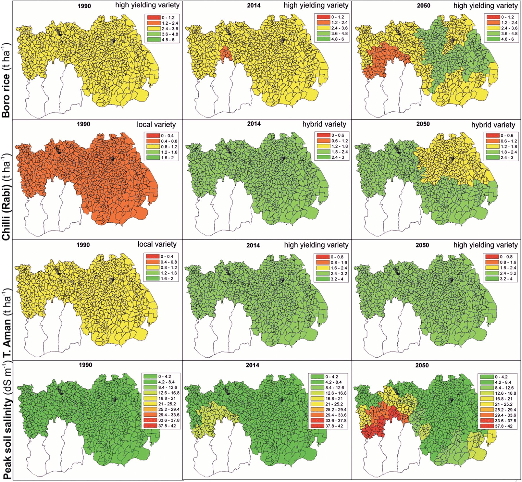 | ||
| Fig. 8 Spatial variation of simulated yield (tons ha−1) only partially influenced by peak soil salinity (dS m−1). | ||
Three crop behaviours were observed in the results. The first type of crop behaviour is illustrated with the Boro rice. The Boro rice is sensitive to salinization because the growth period is under the highest soil salinity period. This is reflected on the productivity maps: higher yields in low salinity areas and lower yields at high salinity areas (see 2050 in Fig. 8). The second crop response type is illustrated with chilli, but also true for grass pea, potato and wheat. The spatial variation of yield depends on the used climate timeseries. The three blocks on the 2050 maps actually refer to the spatial coverage of the input climate time series (North-West, North-East, South-East). This is an artefact of the model setup and can be resolved if climate data are inputted with a finer spatial scale. Nevertheless, this indicates that these crops are sensitive to the temperature variations (i.e. they are irrigated, thus rainfall and evaporation has little effect on them). The third crop response type includes transplanted Aman rice. This is a well-suited crop in the study area, having uniform yield values that are quite close to potential. It is grown in the low salinity period and is not sensitive to temperature changes, thus potentially having present and future significance in coastal Bangladesh. Beside these three basic crop types, Aus rice sits somewhere in between Boro and T. Aman: it has generally high yields everywhere in the study area, where the salinity levels are low. However, when the salinity levels become too high, Aus yields immediately become lower.
(e) Changing demography and agriculture livelihoods
The observed 1991–2011 population numbers and the projected population change (2012–2050) of the coastal zone are shown in Fig. 9. While the population is still large, the population is relatively stable and expected to fall. The rapid increase in population during the 1990–2001 period is followed by a gentle population increase until 2011. Generally a low fertility rate in the study area contributes to the population decrease in most districts through a fall in the number of children. This decreased population is further intensified by outmigration from the North-East part of the study area. Therefore, the population projections show Bangladesh continuing on the demographic transition from a rural economy towards a more urban and service-based economy over the next 50 years.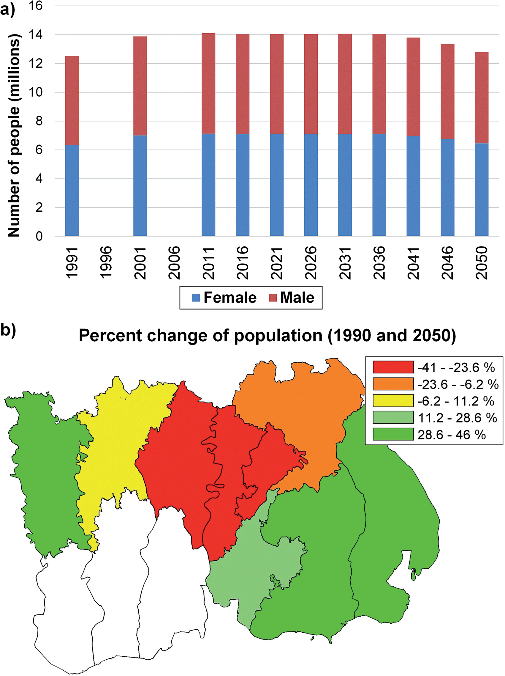 | ||
| Fig. 9 Overall population is stable (a), but internal migration does occur (b). Note, the Sunderbans is assumed to have no population. | ||
A decreasing population has various implications in agriculture. There will be less pressure on the land available, although the ability of the poor to purchase land, even if it does become available, is low. If there is a higher urban population, this means that more food will have to be produced for transport and trade, rather than for subsistence or local consumption. A lower population, however, may also mean a shortage of labour for agricultural production, but in reality there are more unemployed people than agricultural labour available, so it may just mean an increase in the wage of those employed in agriculture. Finally, the low number of children and high outmigration rates will mean that less support is available for the elderly, thus a structural change can be expected for the whole society.
The model aims to incorporate future population projection methods and a simplified representation of land availability for farming agents. Modelling societal changes are extremely difficult and are outside the aims of the paper. Although the population projection method is not linked to the livelihood changes in the current version, it allows the testing of different scenario assumptions, and thus facilitates mapping the uncertainties of the simulations.
(f) Livelihoods from traditional and progressive farming
Crop productivity defines the revenue of farmers, but farmers' livelihoods are also affected by the associated costs. Depending on the cropping pattern chosen by the farmer, their income level and thus their quality of life are affected. The progressive farming uses short duration vegetables instead of Boro rice, thus these vegetables are less affected by salinity (Fig. 7) and they also have a higher market price (in 2013, rice: 17 BDT per kg, chilli: 33 BDT per kg). Thus they can be lucrative if the climate conditions are favourable and sufficient and good quality irrigation water is available. Furthermore, vegetables generally require fewer seeds and have a higher potential yield. Thus, they have the potential to significantly increase the revenues of the both land owners and labourers (through higher labour demand). The simulations show that although progressive farming can be very lucrative, traditional farming provides a more predictable livelihood (Fig. 10). The year-to-year variability of the net earnings from the progressive farming is striking. The variation shown in Fig. 10 is not caused by model instability but indicates higher risks for the land owner in some years. The Aus and Aman rice mitigate the net earning losses in the simulations, but the higher associated costs of vegetables quickly eliminate the profit in a bad year. The model results indicate the sensitivity of vegetables to climatic changes, predominantly to air temperature (see Table 3). This might not be the case in the study area and could be caused by the sensitivity of the CROPWAT model to temperature changes. This requires further validation by field data, but currently no other data are available for additional tests. The traditional, rice-based farming demonstrates less inter-annual variability in the simulations, and thus can be considered more risk tolerant. This might be another reason why the poorest households practice staple-food-based farming: lower net profit, but less upfront costs and lower risk. The poorest populations are often risk averse, choosing survival over the opportunity to increase income.50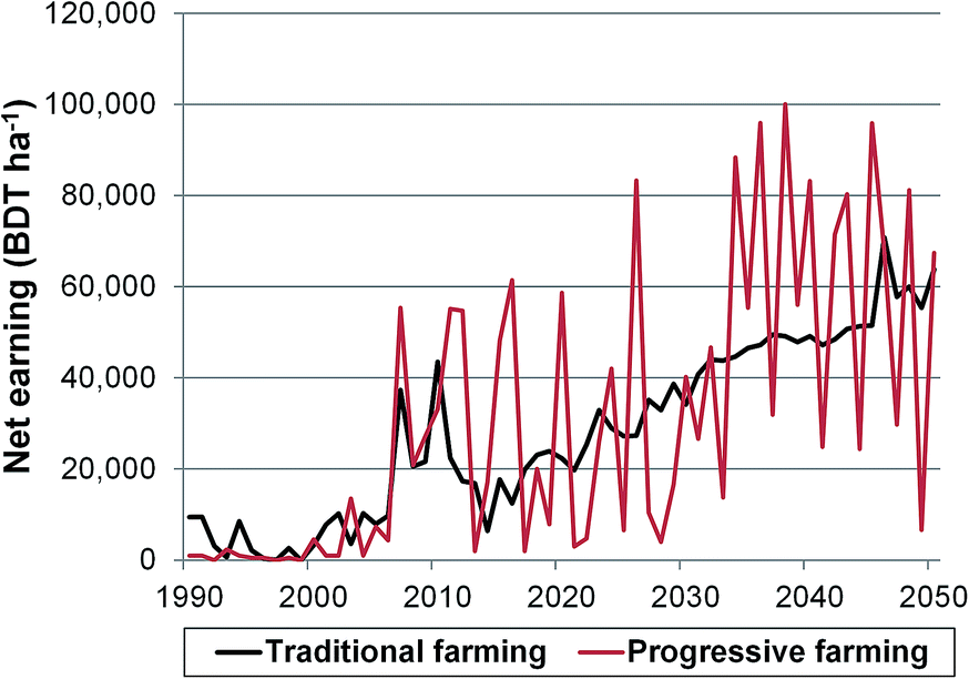 | ||
| Fig. 10 Progressive farming is often more profitable, but traditional farming is more predictable. | ||
(g) Agriculture and informal loans
Fig. 10 shows that the market conditions were not ideal for the land owners during the 1990–2005 period (i.e. negligible profit). In this period, agriculture costs were higher than farm-related income, thus all simulated agents required both official and informal loans during the simulation period. The profit from agriculture was not sufficient during the 60 year-long simulation to pay back the loans completely, thus all agents were caught in the cycle of debt. However, while loan related expenses were around 70 percent of the total household expenses for large land owners, the loan expense was roughly 95 percent for the other agents (small land owners, sharecroppers, landless labourers) on average.The household livelihood model used is simple, yet it is capable of showing the impact of economic, climate and environmental changes on people's livelihoods. The model uses a number of assumptions such as the unconditional availability of loans. This does not represent reality and yet, the simulated agents do end in a poverty trap. Such simulations can inform decision makers about the importance of sensible economic (e.g. better loan availability/conditions and subsidies), research (e.g. new resilient crop varieties) and educational incentives (e.g. new cropping patterns) that can support the rural poor in the face of climate and environmental changes.
(h) Farming and poverty
The current integrated model only considers farm-related revenues. Fig. 11 shows that only doing farming does not make people richer even if climate change naturally improves crop productivity through CO2 fertilisation. Rather, farmers are forced to do other, off-farm jobs to support their families. Fig. 11a indicates a counter-intuitive relative wealth (i.e. smaller number of months with sub-optimal food consumption) for the initial 10–15 years of the low profitability period. During this period, the agents quickly consumed any savings and took official and informal loans and their simulated diet changed from normal to suboptimal as indicated by the increasing number of months per year when the calorie intake was lower than 2122 kcal per capita per day. Traditional farming mitigated the situation to some extent for the large land owners, but eventually, all simulated agents became poor due to the cycle of debt. The model shows that if economic conditions do not change (including loan types), all simulated farmers are expected to be squeezed by falling prices for their produce (compared to total household expenses), and a lack of flexibility to take up alternative income sources because they have to look after their own land. Interestingly, the progressive cropping pattern scenario offers a way out of the situation by slowly reducing the length of the hunger period after 2035. Landless agents are better-off than small land owners and sharecroppers in this simulation, because they do not have to make an investment and their labour wage is ‘guaranteed’. Therefore, while land ownership provides income security to rural populations, especially by meeting subsistence needs and providing some food security, its impact is limited in the face of increasing variability in crop productivity under climate and market changes. | ||
| Fig. 11 Although income-based poverty indicator (b) shows reduced poverty levels, the food-security indicator (a) highlights hardship. | ||
When the monetary poverty is calculated (US$1.25, PPP adjusted, poverty threshold that only considers farm-related incomes), the picture is very different (Fig. 11b). On average, simulated poverty levels are reduced from 90 percent to 60 percent but the reduction trend stopped around 2003. The uncertainty band is relatively narrow due to the fact that only the CROPWAT model parameter uncertainties are considered on this figure. Economic data and the uncertainties of the household livelihood model are currently not included in the model. The narrow band of uncertainty indicates that even though the large variability can be expected in future crop productivities and farm related profits; it is probable that the coastal population will be poor if only faming is practiced. The uncertainties do not increase over time because the annual crop calculations can be considered independent (see Section 4a).
Rural poverty levels are often higher than the national average. By considering that the simulations only use farm-related revenues and the fact that the study site is primarily a remote rural area, the simulation results are comparable with the World Bank data (Fig. 11b). The observed national level poverty levels were 70 percent and 43 percent in 1992 and 2010, respectively, whereas the corresponding poverty levels obtained from our model were 90 percent and 64 percent. However, this monetary indicator only uses the household incomes and does not consider the total expenses, thus painting a too rosy picture about the well-being of the population. Therefore, such monetary poverty indicators are only recommended for policy decision making, if they are accompanied by poverty indicators that capture other sides of well-being (nutrition, health, education, etc.).
Conclusions
An integrated framework and model is being developed within the ESPA Deltas (Assessing Health, Livelihoods, Ecosystem Services and Poverty Alleviation in Populous Deltas) project to investigate the effect of climatic and environmental change on poverty and health of the rural population of coastal Bangladesh. Four essential modelling blocks were identified to capture farm-related livelihood dynamics: (1) crop simulation, (2) demographic projections at the local scale, (3) household livelihood model and (4) carefully selected poverty indicators. Scale is a critical element in the integration. Different elements of the system require the simulation at different spatial (from union to division) and temporal (from daily to 10-yearly) scales, but these are harmonised to enable the communication of model elements. The final outputs of the model are represented at union (28 km2 on average) and monthly scales. These are the most appropriate scales for decision makers, because (i) unions are the smallest planning units in Bangladesh, (ii) unions capture the fine spatial variations of environmental factors and land use changes, (iii) monthly analysis highlights seasonality issues, and (iii) the well-being results are meaningful without becoming computationally very expensive.This paper focused on agriculture and agriculture-related livelihoods using a novel setup for the extended CROPWAT model. A thorough sensitivity analysis was carried out that highlighted the importance of the seasonality in parameter sensitivity. Furthermore, the integrated model was developed to automatically carry out the uncertainty analysis during the normal model runs, based on the most sensitive crop parameters, and their statistical summary was propagated through the livelihood and poverty calculations. The ensemble members of this uncertainty analysis were also analysed to learn about the behaviour of the extended CROPWAT model. Such an integrated assessment across bio-physical and social science domains is uncommon, but makes the scenario results relevant to stakeholders.
The model presented here is capable of providing important insights into the complex relationship of nature, livelihood, poverty and health. It was demonstrated that the relationship between increases in productivity and increases in rural wellbeing is complex and non-linear. However, some key preliminary outcomes should be highlighted. Firstly, an increase in productivity translates into only a slight increase in income for farmers and even a large increase in income cannot guarantee reduced poverty levels due to accrued debt. This highlights a potential issue of rural economics that needs to be addressed in Bangladesh relating to access to affordable and official credit and demonstrates that credit itself, often cited as a way to help the rural poverty, can actually drive households further into poverty. Secondly, the majority of rural households are landless, and based on the simulations, the number of landless is expected to increase. These households are involved in agricultural labour, but may receive the majority of their income from off farm sources. Thirdly, crop diversification does not guarantee a solution to a changing climate unless it is guided with research and development activities and knowledge transfer. Finally, to assess this complex behaviour of people and to understand the lives of rural households, integrated models are necessary that look beyond national economic indicators. Traditional economy-based indicators are useful to measure national progress, but to understand the well-being of people a more disaggregated approach is needed together with targeted indicators measuring important non-monetary aspects of life such as health and education.
This paper has provided insights into the livelihood changes of farmers that may occur as a result of climate and environmental change using an innovative prototype model. In addition, by exploring plausible scenarios, the model development and the analysis of results promote multi-disciplinary co-operation and discussions within the research community and stakeholders. Even though the model elements presented in this paper are simplified representations of both agricultural and population changes, the model produces realistic portrayals and provides a unique platform to explore the links between demographical, climate and environmental changes and their cumulative effect on farming livelihoods and poverty levels in coastal Bangladesh. The model is going to be further developed and extended as more modelled and field data become available from the ESPA Deltas project. This will include incorporating a soil salinity model (based on river and groundwater salinity and farm management), including fishing, livestock and resource collection livelihoods, and further development of the household livelihood model with feedback on land cover/land use and migration. Despite its limitations, the model provides a unique platform to explore the links between demographical and climate changes on agriculture and their cumulative effect on farming livelihoods and poverty levels in not only coastal Bangladesh, but also in other coastal deltas.
Acknowledgements
The authors are grateful to Dr Md. Abdur Rashid (Bangladesh Agricultural Research Institute) for providing agro-economic data. This work ‘Assessing Health, Livelihoods, Ecosystem Services and Poverty Alleviation in Populous Deltas’ (NE-J002755-1)’ was funded with support from the Ecosystem Services for Poverty Alleviation (ESPA) programme. The ESPA programme is funded by the Department for International Development (DFID), the Economic and Social Research Council (ESRC) and the Natural Environment Research Council (NERC). The authors also acknowledge the use of the IRIDIS High Performance Computing Facility, and associated support services at the University of Southampton, in the completion of this work.Notes and references
- J. D. Milliman, J. M. Broadus and F. Gable, Ambio, 1989, 18, 340–345 Search PubMed.
- J. Pender, in Forced Migration Review, 2008, pp. 54–55 Search PubMed.
- BBS, Yearbook of Agricultural Statistics of Bangladesh, Statistics and Informatics Division, Ministry of Planning, Government of the People’s Republic of Bangladesh, Bangladesh Bureau of Statistics, 2011 Search PubMed.
- D. C. Roy, in Climate Change and Migration: Rethinking Policies for Adaptation and Disaster Risk Reduction, ed. M. Leighton, X. Shen and K. Warner, United Nations University Institute for Environment and Human Security, SOURCE ‘Studies of the University: Research, Counsel, Education’ Publication Series of UNU-EHS No. 15/2011, 2011 Search PubMed.
- Z. Islam, Bangladesh Environment, 2000, 596–606.
- S. B. Murshed, A. S. Islam and M. S. A. Khan, in 3rd International Conference on Water & Flood Management (ICWFM 2011), 2011 Search PubMed.
- M. Walsham, Assessing the Evidence: Environment, Climate Change and Migration in Bangladesh (ENG0111), International Organization for Migration (IOM), 2010 Search PubMed.
- H. Brammer, Climate Risk Management, 2014, 1, 51–62 CrossRef PubMed.
- J. Pethick and J. D. Orford, Global Planet. Change, 2013, 111, 237–245 CrossRef PubMed.
- NIPORT, MEASURE, UNC and ICDDRb, Bangladesh Urban Health Survey 2013-Preliminary Results, National Institute of Population Research and Training (NIPORT); MEASURE Evaluation; UNC-Chapel Hill; International Centre for Diarrhoeal Disease Research, Bangladesh, 2014.
- GED, Perspective Plan of Bangladesh: Making Vision 2021 a Reality, General Economics Division, Planning Commission, Government of the People’s Republic of Bangladesh, 2012 Search PubMed.
- G. B. Hall, N. W. Malcolm and J. M. Piwowar, Trans. GIS, 2001, 5, 235–253 Search PubMed.
- A. Li, A. Wang, S. Liang and W. Zhou, Ecol. Modell., 2006, 192, 175–187 CrossRef PubMed.
- T. E. S. Bontkes, Syst. Dynam. Rev., 1993, 9, 1–21 CrossRef PubMed.
- Q. J. Zhao and Z. M. Wen, Procedia Environ. Sci., 2012, 13, 1383–1394 CrossRef PubMed.
- J. Forrester, R. Greaves, H. Noble and R. Taylor, Complexity, 2014, 19, 73–82 CrossRef PubMed.
- P. H. Verburg, A. Veldkamp, L. Willemen, K. P. Overmars and J.-C. Castella, in Ecosystems and Land Use Change, American Geophysical Union, 2013, pp. 217–230 Search PubMed.
- A. Castelletti and R. Soncini-Sessa, Environ. Model. Software, 2007, 22, 1075–1088 CrossRef PubMed.
- O. Varis and M. Keskinen, Int. J. Water Resour. Dev., 2006, 22, 417–431 CrossRef PubMed.
- M. A. Abedin, U. Habiba and R. Shaw, in Environment Disaster Linkages, ed. R. Shaw and T. Phong, Emerald Publishers, UK, 2012, vol. 9, pp. 165–193 Search PubMed.
- BIDS, Financial Implications for Food Security Interventions in the Context of Climate Change in Bangladesh, Bangladesh Institute of Development Studies, E-17 Agargaon, Sher-e Bangla Nagar, Dhaka-1207, 2013 Search PubMed.
- R. Rahman and M. S. Mondal, in Food Security and Risk Reduction in Bangladesh, ed. U. Habiba, A. W. R. Hassan, M. A. Abedin and R. Shaw, Springer, Japan, 2015, pp. 213–234 Search PubMed.
- FAO, Bridging the Rice Yield Gap in Bangladesh, Food and Agriculture Organization of the United Nations, Regional Office for Asia and the Pacific, Bangkok, Thailand, 2000 Search PubMed.
- FAO, CLIMWAT 2.0 for CROPWAT, 2014, http://www.fao.org/nr/water/infores_databases_climwat.html, accessed 15 May 2014 Search PubMed.
- S. N. Mitra, M. Nawab Ali, S. Islam, A. R. Cross and T. Saha, Bangladesh Demographic and Health Survey, 1993-1994, National Institute of Population Research and Training (NIPORT), Mitra and Associates and Macro International Inc., Calverton, Maryland, 1994 Search PubMed.
- NIPORT, Mitra and ICF, Bangladesh Demographic and Health Survey 2011, National Institute of Population Research and Training (NIPORT), Mitra and Associates and ICF International, Dhaka, Bangladesh and Calverton, Maryland, USA, 2013 Search PubMed.
- WRI, World Resources 2005: The Wealth of the Poor—Managing Ecosystems to Fight Poverty, World Resources Institute in collaboration with United Nations Development Programme, United Nations Environment Programme, and World Bank 2005, WRI, Washington, DC, 2005 Search PubMed.
- A. Rahman, A. Mozaharul, K. Mainuddin, M. L. Ali, S. M. Alauddin, M. G. Rabbani, M. M. U. Miah, M. R. Uzzaman and S. M. A. Amin, Policy Study on the Probable Impacts of Climate Change on Poverty and Economic Growth and the Options of Coping with Adverse Effect of Climate Change in Bangladesh, General Economics Division, Planning Commission, Government of the People’s Republic of Bangladesh & UNDP Bangladesh, 2009 Search PubMed.
- H. Wright, P. Kristjanson and G. Bhatta, Understanding Adaptive Capacity: Sustainable Livelihoods and Food Security in Coastal Bangladesh, Working Paper No 32, CGIAR Research Program on Climate Change, Agriculture and Food Security, 2012 Search PubMed.
- K. A. Toufique and C. Turton, Hands Not Land: How Livelihoods Are Changing in Rural Bangladesh, Bangladesh Institute of Development Studies, 2002 Search PubMed.
- J. Caesar, T. Janes, A. Lindsay and B. Bhaskaran, Environ. Sci.: Processes Impacts, 2015 10.1039/C4EM00650J.
- KNMI, KNMI CLimate Explorer: SRES A1B CO2 concentrations (1985-2100), 2014, http://climexp.knmi.nl/data/iA1B.dat, accessed 15 May 2014 Search PubMed.
- M. S. N. Islam and A. Gnauck, in Proceeding of WWW-yes Workshop in University of Paris Est from 29th May–5th June 2010, Paris, France, 2010, pp. 153–163 Search PubMed.
- M. Ahsan, Saline Soils of Bangladesh, Soil Resource Development Institute, Ministry of Agriculture, Farmgate, Dhaka, Bangladesh, 2012 Search PubMed.
- D. Clarke, M. Smith and K. El-Askari, Irrig. Drain., 1998, 47, 45–58 Search PubMed.
- R. G. Allen, L. S. Pereira, D. Raes and M. Smith, FAO Irrigation and Drainage Paper – no. 56: Crop Evapotranspiration (Guidelines for Computing Crop Water Requirements), FAO, Water Resources, Development and Management Service, Rome, Italy, 1998 Search PubMed.
- D. Raes, P. Steduto, T. C. Hsiao and E. Fereres, AquaCrop Version 4.0: Chapter 3 Calculation Procedures, FAO, Land and Water Division, Rome, Italy, 2012 Search PubMed.
- BBS, Report on Sample Vital Registration System – 2010, Statistics Division, Ministry of Planning, Government of the People’s Republic of Bangladesh, Bangladesh Bureau of Statistics, 2011 Search PubMed.
- UN, World Population Prospects, the 2012 Revision, 2012, http://esa.un.org/wpp/unpp/panel_indicators.htm, accessed 18 November 2012 Search PubMed.
- BBS, SID and MP, Population and Housing Census 2011. Socio-economic and Demographic Report, Bangladesh Bureau of Statistics, Statistics and Informatics Division, Ministry of Planning, 2012 Search PubMed.
- BBS, Statistical Yearbook of Bangladesh – 2010, Statistics Division, Ministry of Planning, Government of the People’s Republic of Bangladesh, Bangladesh Bureau of Statistics, 2011 Search PubMed.
- I. J. Bateman, A. R. Harwood, G. M. Mace, R. T. Watson, D. J. Abson, B. Andrews, A. Binner, A. Crowe, B. H. Day, S. Dugdale, C. Fezzi, J. Foden, D. Hadley, R. Haines-Young, M. Hulme, A. Kontoleon, A. A. Lovett, P. Munday, U. Pascual, J. Paterson, G. Perino, A. Sen, G. Siriwardena, D. van Soest and M. Termansen, Science, 2013, 341, 45–50 CrossRef CAS PubMed.
- BBS, Report of the Household Income & Expenditure Survey 2010, Bangladesh Bureau of Statistics, Statistical Division, Ministry of Planning, 2011 Search PubMed.
- M. S. Mondal, A. F. M. Saleh, M. A. Razzaque Akanda, S. K. Biswas, A. Z. M. Moslehuddin, S. Zaman, A. N. Lazar and D. Clarke, Environ. Sci.: Processes Impacts, 2015 10.1039/C5EM00095E.
- S. S. Myers, A. Zanobetti, I. Kloog, P. Huybers, A. D. B. Leakey, A. J. Bloom, E. Carlisle, L. H. Dietterich, G. Fitzgerald, T. Hasegawa, N. M. Holbrook, R. L. Nelson, M. J. Ottman, V. Raboy, H. Sakai, K. A. Sartor, J. Schwartz, S. Seneweera, M. Tausz and Y. Usui, Nature, 2014, 510, 139–142 CrossRef CAS PubMed.
- FAO, FAOSTAT Dataset: Emissions – Agriculture, http://faostat3.fao.org/browse/G1/*/E Search PubMed.
- D. Clarke, S. Williams, M. Jahiruddin, K. Parks and M. Salehin, Environ. Sci.: Processes Impacts, 2015 10.1039/C4EM00682H.
- A. M. S. Ali, Land Use Pol., 2006, 23, 421–435 CrossRef PubMed.
- M. H. Rahman, T. Lund and I. Bryceson, Ocean Coast Manag., 2011, 54, 455–468 CrossRef PubMed.
- J. C. Scott, The Moral Economy of the Peasant: Rebellion and Subsistence in Southeast Asia, Yale University Press, 1977 Search PubMed.
Footnote |
| † Electronic supplementary information (ESI) available: Description about the extended CROPWAT model and its application within this research. See DOI: 10.1039/c4em00600c |
| This journal is © The Royal Society of Chemistry 2015 |