Important issues facing model-based approaches to tunneling transport in molecular junctions†
Received
5th May 2015
, Accepted 8th July 2015
First published on 8th July 2015
Abstract
Extensive studies on thin films indicated a generic cubic current–voltage I–V dependence as a salient feature of charge transport by tunneling. A quick glance at I–V data for molecular junctions suggests a qualitatively similar behavior. This would render model-based studies almost irrelevant, since, whatever the model, its parameters can always be adjusted to fit symmetric (asymmetric) I–V curves characterized by two (three) expansion coefficients. Here, we systematically examine popular models based on tunneling barriers or tight-binding pictures and demonstrate that, for a quantitative description at biases of interest (V slightly higher than the transition voltage Vt), cubic expansions do not suffice. A detailed collection of analytical formulae as well as their conditions of applicability is presented to facilitate experimentalist colleagues to process and interpret their experimental data obtained by measuring currents in molecular junctions. We discuss in detail the limits of applicability of the various models and emphasize that uncritically adjusting the model parameters to experiment may be unjustified because the values deduced in this way may fall in ranges rendering a specific model invalid or incompatible to ab initio estimates. We exemplify with the benchmark case of oligophenylene-based junctions, for which the results of ab initio quantum chemical calculations are also reported. As a specific issue, we address the impact of the spatial potential profile and show that it is not notable up to biases V ≳ Vt, unlike at higher biases, where it may be responsible for negative differential resistance effects.
1 Introduction and background
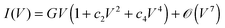
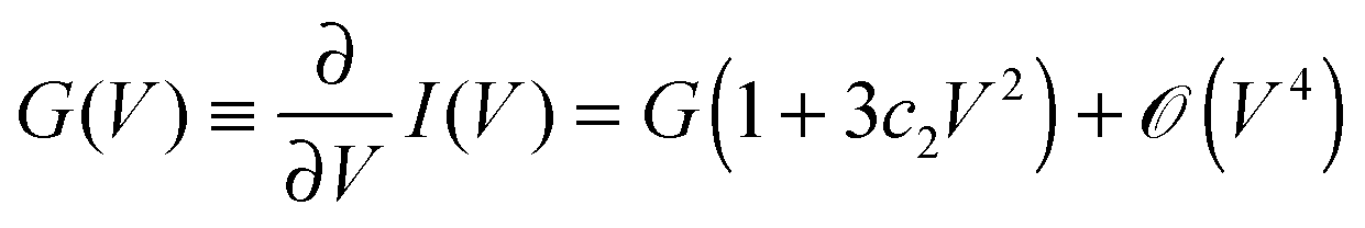
The roughly parabolic shape of the conductance G(V) ≡ ∂I/∂V, or the related cubic dependence of the current (I) on bias (V), was considered a prominent characteristic of transport via tunneling. This conclusion emerged from extensive studies on a variety of macroscopic thin film junctions of oxides, insulators, superconductors up to relatively large biases.1–6 A quick glance at I–V measurements in a variety of molecular junctions may convey the impression that this cubic dependence is satisfactory also for such systems.7 As an illustration, we have chosen in Fig. 1a a measured I–V curve,8 for which fitting with a cubic polynomial looks particularly accurate. The view based on such third-order Taylor expansions (cf.eqn (1)) was able to qualitatively describe a series of interesting aspects related to charge transport in molecular junctions.9
| |  | (1) |
 |
| | Fig. 1 (a) Fitting the red I–V curve measured for a CP-AFM Ag/OPD1/Ag molecular junction8 with a cubic polynomial, eqn (1), depicted by the blue line may appear to be quite satisfactory. (b) Nevertheless, for the same curves, the difference in the positions of the minimum of the Fowler–Nordheim (FN) quantity log(I/V2) defining the transition voltage Vt is substantially larger than experimental uncertainties (δVt < 0.1 V![[thin space (1/6-em)]](https://www.rsc.org/images/entities/char_2009.gif) 8). In the case illustrated here, the transition voltage obtained viaeqn (1) is even beyond the bias range accessed experimentally. (c) As an alternative to the FN plot, one can inspect a “peak voltage spectrum”, namely the quantity V2/I plotted vs. V,14 which exhibits a maximum located at V = Vt. (We show only the range V > 0 because the measured I–V curve is symmetric to a very good approximation.). 8). In the case illustrated here, the transition voltage obtained viaeqn (1) is even beyond the bias range accessed experimentally. (c) As an alternative to the FN plot, one can inspect a “peak voltage spectrum”, namely the quantity V2/I plotted vs. V,14 which exhibits a maximum located at V = Vt. (We show only the range V > 0 because the measured I–V curve is symmetric to a very good approximation.). | |
Above,  is the low bias conductance.10
However, if the approximation of eqn (1) were quantitatively adequate, it would be deceptive for a model-based description of transport in molecular junctions. Resorting to simple phenomenological models enabling expedient data processing and interpretation of charge transport through nanoscale devices represents common practice in molecular electronics. The validity of a certain model/mechanism for transport in a given system/device is often assessed by considering its ability to fit the measured current–voltage I–V curves. Adopting this “pragmatic” standpoint, the problem encountered is that an approximate generic parabolic shape of the conductance could be inferred at not too high biases regardless of the tunneling model.7,9 Whether the electron wave function tunnels across a structureless average medium modeled as a tunneling barrier or through tails of densities of states of one (frontier) or a few off-resonant molecular orbital levels, one could “appropriately” adjust a few parameters, and the third-order expansion of the current formula, I = I(V), often available in closed analytical forms from literature,1,3,4,6,11,12 could relatively easily be “made” to fit the usually featureless I–V curves measured. Then the quality of the fitting alone cannot be invoked in favor of one tunneling mechanism out of other possible mechanisms underlying the various phenomenological models.
The inspection of Fig. 1a may indeed convey the impression of an overall very good agreement between experiment and eqn (1). However, a more careful analysis reveals that the range of the highest biases that can be sampled experimentally is quantitatively not so satisfactorily described. Typically, these V-values are only slightly larger than the transition voltage Vt.13 The difference in Vt-values extracted from the experimental and fitting curves of Fig. 1b exceeds typical Vt-experimental errors.
The range V ∼ Vt is of special interest. As discussed in Section 2, Vt represents an intrinsic property of a junction out of equilibrium; it characterizes the (high) bias range exhibiting significant nonlinearity. Therefore, even more than an overall fitting of I–V transport data, it is important for theory to correctly understand/reproduce Vt. And, as illustrated in Fig. 1b and c, to this aim, the theoretical description should go beyond the cubic expansion framework provided by eqn (1). Emphasizing this aspect in the analysis of the various transport models considered below, which are among the most popular in the molecular electronics community,1–3,5,6,11,15–17 represents one main aim of the present study.
Emerging from the idealized description of reality, the models utilized in transport studies, like those used elsewhere, inherently have a limited validity. The various model parameter values are subject to specific restrictions, which represent intrinsic limitations for the model in question; merely succeeding to provide good quality data fitting is meaningless if the parameter values deduced in this way fall outside the range of model's validity. In some cases, these conditions of validity simply reflect restrictions on parameter values justifying certain mathematical approximations made to express a certain result in closed analytical form. Checking whether the various parameters deduced from data fitting do indeed satisfy the corresponding (mathematical) restrictions or are consistent with ab initio estimated values is absolutely necessary. Nevertheless, not rarely current data analysis misses this important consistency step, which may be related to an insufficient discussion in the literature of the physical background of the various phenomenological models and the limited validity of the pertaining analytical formulae. Exposing the limits of applicability of such models frequently used in molecular electronics represents another aim of the present paper. In doing that, this paper is intended as an effort to make the community more aware of these limitations. It should by no means be understood as challenging the utility of model-based studies in gaining valuable conceptual physical insights into charge transport.
Throughout, we will consider the case of zero temperature, as appropriate for off-resonant tunneling and symmetric coupling to electrodes (equal width parameters ΓL = ΓR = Γ due to “left” and “right” electrodes). In agreement with the fact that conductances of typical molecular junctions are much smaller than the quantum conductance G ≪ G0 = 2e2/h = 77.48 μS, we will assume throughout Γs much smaller than relevant (molecular orbital) energy offsets relative electrodes' Fermi energy εB ≡ EB − EF (EF ≡ 0). We will further assume εB > 0, because, for tunneling barriers, the corresponding formulae are simpler to write for electrons (n-type conduction); in all formulae presented below, εB should be understood as |εB| in cases of holes (p-type conduction) tunneling across negative barriers, as easily obtained by performing the charge conjugation transformation (εB = EB − EF → EF − EB = −εB, e → −e, m → −m, see, e.g., ref. 18). Likewise, since the tight-binding Hamiltonians of eqn (S1) and (S3) (ESI†) are invariant under particle-hole conjugation (e.g.ref. 19 and citations therein), the results for +εB and −εB coincide.
While discussing in general the aspects delineated above, we will examine the benchmark case of conducting probe atomic force microscope (CP-AFM) molecular junctions based on oligophenylene dithiols (OPDs)8 as a specific example.
2 Physical properties envisaged
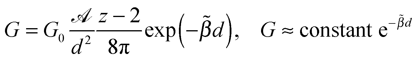
In this paper, we will mainly consider two physical properties (zero-bias conductance G and transition voltage Vt13) and focus our attention on how these properties vary with the molecular length d or size N across homologous series of molecules described within schematic models. Typical for nonresonant tunneling transport is a dependence| | G ∝ exp(−βN) = exp(−![[small beta, Greek, tilde]](https://www.rsc.org/images/entities/i_char_e10e.gif) d) d) | (2) |
where β () characterizes the exponential decay of the zero-bias conductance G with the molecular size (length).
“Historically”,13 the transition voltage Vt was introduced as the bias at the minimum of the Fowler–Nordheim quantity log(I/V2); the initial claim was that of a mechanistic transition from direct tunneling across a trapezoidal energy barrier (V < Vt) to Fowler–Nordheim (field-emission) tunneling across a triangular barrier (V > Vt).13 As already noted in previous studies,17,20,21 such a Fowler–Nordheim transition does not occur in molecular junctions. Physically, Vt has nothing to do with the Fowler–Nordheim tunneling theory.22–24 In particular, in molecular junctions the quantity log(I/V2) does not linearly decrease with 1/V at higher biases; this was a result deduced for the extraction of electrons from cold metals by intense electric fields.23
Still, transport measurements in molecular junctions do yield curves for log(I/V2) exhibiting a minimum. Mathematically, the bias V = Vt at the minimum of log(I/V2) coincides with the bias where the differential conductance is two times larger than the nominal conductance25
| |  | (3) |
Eqn (3) can be taken as an alternative mathematical definition of
Vt revealing at the same time its physical meaning. Using the minimum of log(
I/
V2) plotted as a function of
V (or 1/
V)
13 merely represents a mathematical trick to extract the
Vt-value of
eqn (3). To eliminate the confusion that continues to exist in the literature on a mechanistic (Fowler–Nordheim) transition occurring at
V =
Vt, instead of Fowler–Nordheim diagrams log(
I/
V2)
vs. V, it might be more appropriate to use diagrams
V2/
I vs. V, which have maxima exactly at the same
V =
Vt given by
eqn (3);
14 so, instead of “transition voltage spectra” (“TVS”,
Fig. 1b), one can speak of a “peak voltage spectra” (“PVS”,
Fig. 1c).
As expressed by eqn (3), Vt represents a genuine nonequilibrium property characterizing the charge transport through a molecular junction out of equilibrium. So, Vt is qualitatively different from the zero-bias conductance G; in fact, the latter (as well as other properties commonly targeted in measurements, e.g., the thermopower Seebeck coefficient) can be expressed by properties of a device (let it be molecular junctions or else) at equilibrium via a fluctuation-dissipation theorem.26 Interestingly, as revealed by recent studies27–29 and supported by measurements comprising thousands of molecular junctions,30,31 it is even more justified to consider Vt (rather than G) as a junction's characteristic property; in a given class of molecular junctions, Vt is much less affected by inherent stochastic fluctuations than individual I–V traces or low bias conductances G.30 The aforementioned should be taken as motivation why Vt represents a quantity on which the present transport study focuses.
3 Models and relevant analytical formulae for symmetric I–V curves
In this section we will examine a series of models widely employed in studies on charge transport through molecular devices. For some of these models, the dependence I = I(V) or other useful formulae can be given in closed analytical form. It is worth remembering that for describing idealized situations, these analytical results hold only if certain conditions are satisfied. Whatever the case, the conditions of validity will also be given below. Other models examined in this paper rely on tight-binding Hamiltonians, for which the exact dependence I = I(V) can be obtained without substantial numerical effort.
For reasons presented later, the expansion coefficients c2 and c4 of the current up to the fifth order, eqn (4), will also be provided for each case
| |  | (4) |
They can be directly inserted into
eqn (5) and (6) to compute the transition voltages
Vt3 and
Vt5 within the third and the fifth order expansion, respectively
| |  | (5) |
| |  | (6) |
Note that the expansion coefficients can be expressed as
where
V2 and
V4 have dimensions of voltages and allow one to express the expansion in terms of dimensionless voltages
Next we briefly describe the models considered here and, whenever possible, give the relevant analytical formulae for the low bias conductance G (G0 ≡ 2e2/h = 77.48 μS is the conductance quantum), the expansion coefficients c2 and c4 entering eqn (4) as well as the transition voltage Vt along with the conditions for their validity.
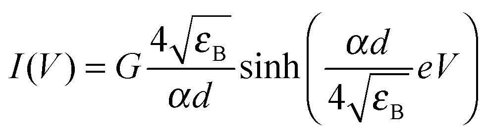
(i) For biases e|V| < εB, within the Simmons WKB-based approximation for electron tunneling across a tunneling barrier of effective height εB without lateral constriction (Simmons's model), the current I is given by eqn (7).1,5 The Taylor expansion of the RHS of eqn (7) allows one to deduce formulae for the zero-bias conductance G and the coefficients c2 and c4 entering eqn (4). They are expressed by eqn (8), (10) and (11), respectively
| |  | (7) |
| |  | (8) |
| |  | (9) |
| |  | (10) |
| |  | (11) |
| |  | (12) |
Above,

stands for the junction's transverse area and
| |  | (13) |

,
m0 and
m* are Sommerfeld's constant,
32 free and effective electron mass, respectively.
Eqn (12) (like
eqn (18) below) defines a dimensionless junction width
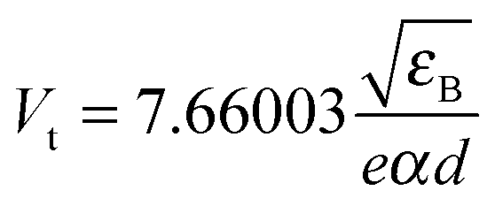
z. The transition voltage for the Simmons and Simmons-based models has been investigated in a series of recent studies.
18,20,25,33–35
Eqn (7) and (8) represent mathematical approximation results; in addition to the restriction on the bias range specified, they only hold for barriers satisfying eqn (12), requiring tunneling barriers sufficiently high and wide.15 In fact, the applicability of Simmons' approximation is more restrictive than required by eqn (12), as revealed by a more detailed analysis.5,36,37
(ii) For electron tunneling across a tunneling barrier with lateral constriction at biases e|V| ≲ εB, the current I can be expressed by eqn (14),18 which applies provided that eqn (18) is satisfied. In addition to the quantities G, c2 and c4 obtained by expanding the RHS of eqn (14), the transition voltage Vt can also be expressed in closed analytical form; see eqn (15), (16) and (17)
| |  | (14) |
| | | G ∝ exp(−d) | (15) |
| |  | (16) |
| |  | (17) |
| |  | (18) |
Noteworthy, the restriction imposed by
eqn (18) to the results of
eqn (14) and (15) is more severe than that expressed by
eqn (12), which refers to a situation less appropriate for molecular electronic devices. Like
eqn (12),
eqn (18) expresses the fact that the above results for model (ii) hold for physical situations where tunneling barriers are sufficiently high and wide.
(iii) The highly off-resonant sequential tunneling11 (the superexchange limit38) across a molecular bridge consisting of a wire with N sites and one energy level (εB) per site represents a limiting case of the situation depicted in Fig. 2a. Provided that eqn (22) is satisfied, the current is expressed by eqn (19), (20) and (21) follow via straightforward series expansion.
| |  | (19) |
| |  | (20) |
| |  | (21) |
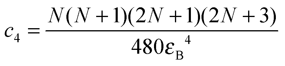
| |  | (22) |
 |
| | Fig. 2 Panels (a) and (b) represent schematically the tight binding models described by eqn (S1) and (S3) (ESI†). Panels (c) and (d) depict the cases of a constant potential and a linear potential drop, respectively, as limiting cases of spatial potential profiles between electrodes under a bias V. | |
Here, th is the hopping integral between the nearest neighboring sites. Eqn (19) and (20) emerge from the Landauer formula, eqn (25), using the transmission given in the RHS of eqn (S2) (ESI†) for arbitrary N. Note that the power dependent transmission expressed by the latter yields a strict proportionality
where the dimensionless quantity
ut is the solution of the parameter-free algebraic
eqn (24), which results by inserting
eqn (19) into
eqn (3)| | | (N − 1/2)ut[(1 + ut)2N + (1 − ut)2N] = (1 − ut)(1 + ut)2N − (1 + ut)(1 − ut)2N | (24) |
Eqn (22) expresses the physical fact that the above results for model (iii) hold for situations corresponding to strongly off-resonant tunneling.
(iv) A molecular chain consisting of N monomers, each monomer being characterized by a single orbital, is schematically depicted in Fig. 2a. Model (iii) presented above represents a limiting case (cf.eqn (22)) of this model. To illustrate this, we give in eqn (S2) of the ESI† the transmission function computed exactly and within the sequential tunneling approximation for the case N = 2. Adapted to oligophenylene chains, εB should be taken as a model for the HOMO energy of an isolated phenylene unit, and th as the coupling between HOMO levels of adjacent rings. (This is the motivation for choosing the subscript h.)
Under applied bias V, two limiting cases can be considered. One limit is that of an applied field completely screened out by delocalized electrons (the “metallic” molecule, Fig. 2c); the potential is constant across the molecule (Vr = 0), and the site energies εrB are the same εrB ≡ εB. Another limit (no screening, the “insulating” molecule) is that of a potential Vr varying linearly from site to site between the values +V/2 and −V/2 at the two electrodes (Fig. 2d), yielding r-dependent on-site energies εrB = εB − eVr.
(v) Molecular wires consisting of six-site rings with a single (π-electron) energy level per site (CH-unit) depicted in Fig. 2b represent a tight-binding description of oligophenylene molecules. The corresponding second-quantized Hamiltonian is given in the ESI.† As illustrated in Fig. 2b, ti and t stand for intra- and inter-ring hopping integrals, respectively.
Although for models (iv) and (v) the dependence I = I(V) cannot be expressed in closed analytical form, it can be easily obtained numerically within the Landauer framework39
| |  | (25) |
Analytical formulae for the transmission function
T(
E) are lengthy even for
Γ much smaller than
εB and
th's,
40,41 so they are of little interest in the present context. The numerical effort to compute
T(
E)
via the Landauer trace formula is insignificant: it consists of a numerical integration and a matrix inversion, which is needed to compute the retarded Green's function.
39
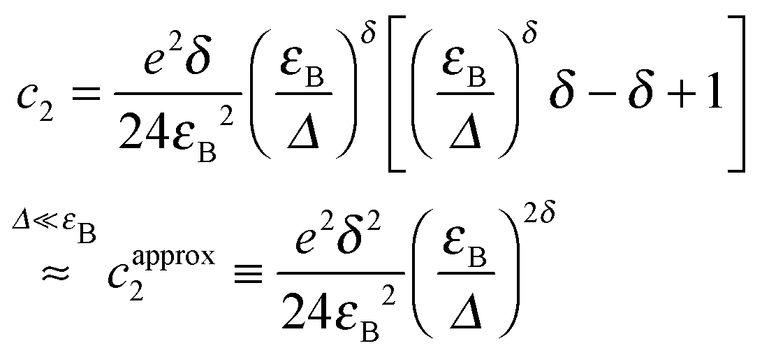
(vi) We will also examine the case of a generalized exponential transmission
| |  | (26) |
The results for this case, including an approximate analytical formula for the current valid for biases not considerably exceeding
Vt and
εB ≫
Δ that can be deduced resorting to a Stratton-like approximation
25,42 for transmission are presented below. The conductance
G in
eqn (29) and the coefficients
c2,4 in
eqn (31) and (32) can be straightforwardly obtained from the fifth-order expansion of the RHS of
eqn (27)| |  | (27) |
| |  | (28) |
| |  | (29) |
| |  | (30) |
| | 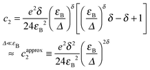 | (31) |
| |  | (32) |
| |  | (33) |
The particular case
δ = 2, which corresponds to a Gaussian transmission, has occasionally been studied in the literature;
9,17 the results for this case are presented in the ESI.
†
The relation given below holds in general (not only for the Gaussian transmission δ ≡ 2)
| | | Vapproxt,5 = 0.797483Vapproxt,3 = 1.02006Vapproxt | (34) |
Here,
Vapproxt,3 and
Vapproxt,5 represent estimates obtained from
eqn (5) and (6) using the approximate coefficients
capprox2 and
capprox4 given above instead of
c2 and
c4, respectively. An expression similar to
Vapproxt,3 has been given previously.
9 Note that the above superscript
approx refers to physical situations of strongly off-resonant tunneling, mathematically expressed by the inequality
Δ ≪
εB.
4 Results for symmetric I–V curves using generic model parameter values
The detailed results for current (I) and transition voltages computed exactly and within the third- and fifth-order expansions (Vt,exact ≡ Vt, Vt,3, and Vt,5, respectively) are collected in Fig. 3–8, Fig. S1–S8 (ESI†). Below we will emphasize some main aspects of the results obtained for the corresponding numerical simulations done using generic parameter values.
 |
| | Fig. 3 The transition voltage Vt,exact computed by using the “exact” current for the Simmons model [termed model (i) in the main text], eqn (7) (panel (a)), along with the approximate estimates Vt,3 and Vt,5 obtained by inserting the expansion coefficients c2 and c4 of eqn (10) and (11) into eqn (5) and (6). Panel (b) shows that, while Vt,3 significantly deviates from Vt,exact (typical experimental uncertainties in Vt do not exceed ∼10%8,31), Vt,5 agrees with Vt,exact within a few percents (z ≡ d is a dimensionless barrier width). | |
 |
| | Fig. 4 (a) The transition voltage Vt,exact computed from the current of eqn (19) corresponding to the superexchange mechanism across a molecular wire modeled as a chain of sites having a single orbital of energy εB [termed model (iii) above], along with the approximate estimates Vt,3 and Vt,5 obtained by inserting the expansion coefficients c2 and c4 of eqn (21) into eqn (5) and (6) (panel (a)). Panel (b) shows that Vt,3 deviates from Vt,exact by up to 73% (much larger than typical experimental uncertainties in Vt of ∼10%8,31), while Vt,5 agrees with Vt,exact within at most 14%. Note that, within the sequential tunneling approximation, Vt,exact, Vt,3, and Vt,5 do not depend on the inter-site hopping integral th. | |
 |
| | Fig. 5 Transition voltage Vt computed exactly for a molecular wire whose monomers are modeled as single sites characterized by a single orbital of energy εB. For arbitrary nearest-neighbor hopping integral values th, this is termed model (iv) in the main text, which becomes model (iii) in the limit th ≪ εB. Note the almost insignificant change Vt → Vt + δVt when the spatial potential profile across the chain changes from constant (Fig. 2c) to a linear drop (Fig. 2d). The differences between the dashed and solid lines in panel (a) represent the absolute changes δVt. The relative changes δVt/Vt are shown in panel (b). | |
 |
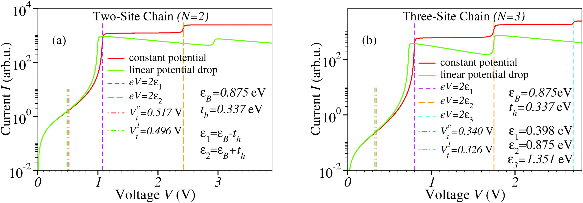
| | Fig. 6 Tunneling current computed for molecular wires [model (iv), eqn (S1), ESI†] for a constant (Fig. 2c) and linearly varying (Fig. 2d) potential. Panels (a) and (b) refer to the cases of two and three sites (N = 2 and N = 3), respectively. The linear potential drop has an impact at higher biases more pronounced than that shown in Fig. S2, S3 and S4 (ESI†); displacements of the current step positions (which are located at on-resonance situations, eV = 2εj, in the case of a constant potential) and negative differential effects. εj's (j ≥ 1) represent the absolute values of the highest occupied orbital energies measured from the electrodes' Fermi energy. For a two-site chain, these values are ε1,2 = εB ∓ th (cf. the inset of panel (a)). Note the logarithmic scale on the y-axis. | |
 |
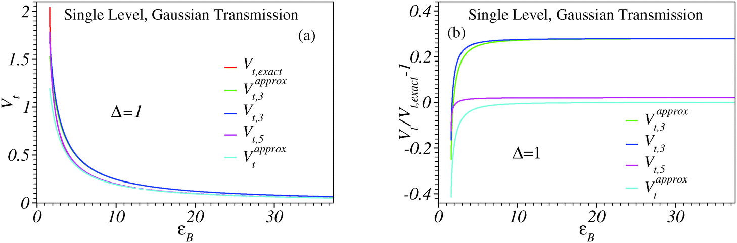
| | Fig. 7 Results obtained using the Gaussian transmission of eqn (S4) (ESI†) showing the dependence on εB of the transition voltage computed exactly (Vt), and using its approximate estimates: Vt,approx of eqn (S7) (ESI†) and Vapproxt,3, Vt,3 and Vt,5 obtained from eqn (5) and (6), (S8) and (S9) (ESI†). Note that both Vapproxt and Vt,5 represent good approximations for large values of the ratio εB/Δ. | |
 |
| | Fig. 8 Results obtained for a Gaussian transmission showing that, while the voltages where the I–V curves (panel (a)) exhibit an inflection point (or maximum of the differential conductance ∂I/∂V of width proportional to Δ, panel (b)) have a dependence similar to the case of a Lorentzian transmission (namely e|V| = 2εB corresponding to the alignment of the energy level εB with the Fermi level of the biased electrodes), the transition voltage decreases with increasing εB, in contrast to the case of Lorentzian transmission, where it increases with εB (eVt = 1.154εB).12 | |
4.1 The need to go beyond the parabolic conductance approximation
As shown in the aforementioned figures, the estimate Vt,5, based on the fifth-order expansion in eqn (4), represents a good approximation for the transition voltage Vt,exact ≡ Vt computed exactly for each model considered. For reasonably broad ranges of the model parameter values, the relative deviations |Vt,5 − Vt|/Vt usually fall within typical experimental errors (≲10%).8,31 This does not apply to the (over)estimate Vt,3, whose deviations from the exact values are considerably larger than experimental errors. As shown in Fig. 4 and Fig. S8 (ESI†), Vt,3 could be almost two times larger than Vt,exact. This demonstrates that the cubic approximation for current (or parabolic approximation for conductance), eqn (1), can only be used for qualitative purposes.
4.2 The spatial potential profile as a possible source of negative differential resistance
The impact of the spatial potential profile across a molecular junction is another issue worthy to be mentioned. Presumably, realistic potential profiles fall between the two situations depicted in panels (c) and (d) of Fig. 2 (a constant potential and a linearly varying potential, respectively); so examining the differences in the results obtained in these two cases may be taken to assess how important is to exactly know the actual potential profile in a real case. The results presented in Fig. S2, S3 and S4 (ESI†) indicate a weak effect at biases not much larger than Vt. Obviously, this is a further plus of transition voltage spectroscopy.
The manner in which the potential varies across a molecular junction is important only at biases substantially higher than Vt. This is shown in Fig. S2, S3 and S4 (ESI†) and especially in Fig. 6, which, to the best of our knowledge, demonstrates a qualitatively new effect. As shown there, instead of a current plateau occurring for a potential flat across the molecule beyond bias values at which molecular orbital energies (ε1,2,…) become resonant to the Fermi level of one electrode (eVres = 2ε1,2,…),39 the current decreases for a linearly varying potential. We are not aware of a previous indication on such a negative differential resistance (NDR) effect related to a specific potential variation across a molecular junction. Noteworthy, this is an NDR effect for uncorrelated transport computed within the limit of wide-band electrodes. Previous work on uncorrelated transport indicated finite electrode bandwidths and energy-dependent electrode density of states as possible sources of NDR.43
4.3 Gaussian transmission versus Lorentzian transmission
The comparison between the cases of Lorentzian (obtained as a particular case of model (iv) for N = 1, discussed in detail previously, e.g., ref. 12) and Gaussian transmission (a particular case of eqn (26)) reveals that even systems wherein the transport is dominated by a single energy level may have qualitatively different physical properties.
As shown in Fig. 7 and Fig. S5 and eqn (S7) (ESI†), Vt strongly depends on the width parameter Δ and is inversely proportional to εB. By contrast, in the case of Lorentzian transmission, Vt linearly increases with εB and is nearly independent of the width parameter Γ as long as  .12,21,29 In fact, both the proportionality to εB and the insensitivity to Γ-variations for Γ ≪ εB are common features shared by the above models (iii–v), while a Vt nearly proportional to εB1/2 at large εB for models (i) and (ii) is the consequence of the fact that the corresponding transmissions are similar to that of eqn (26) with δ = 1/2 (cf.eqn (17) and (30)). Common features for these two types of transmissions are the inflection point of the I–V curves (“current steps”, Fig. 8a) located at biases Vres = 2εB/e where the level becomes resonant to electrodes' Fermi energy, and the fact that the associated maximum in the differential conductance has a width proportional to the transmission widths; δVres ∝ Δ (Fig. 8b), similar to δVres ∝ Γ for Lorentzian transmission. The opposite dependence of Vt on εB for Lorentzian (Vt ∝ εB) and Gaussian (Vt ∝ 1/εB) transmission is relevant for the correctly interpreting gating effects44–46 or the impact of electrodes' work function.27
Concerning the approximate estimates for Vt,exact, Fig. 7b and Fig. S5b (ESI†) indicate a behavior similar to that found in the above cases: Vt,5 represents an accurate estimate for the exact Vt,exact, while Vt,3 is quantitatively unsatisfactory.
5 Asymmetric I–V curves described within the Newns–Anderson model
Let us briefly examine the case where, unlike those assumed throughout above, the I–V curves are not symmetric under bias reversal, i.e., I(−V) ≠ −I(V). It is clear that the asymmetry with respect to bias polarity reversal cannot be satisfied within the framework provided by eqn (1) and (4); even powers in V should also be added| |  | (35) |
| |  | (36) |
By including only the lowest even power (i.e. c1 ≠ 0 and c3 = 0),9 it is possible to account for an asymmetry I(V) ≠ −I(−V). However, doing this, i.e. using eqn (35), has an important drawback. By inserting eqn (35) into eqn (3) one easily obtains| |  | (37) |
i.e., transition voltages of equal magnitudes for positive and negative bias polarities, and this holds no matter how large c1 is. Noteworthily, the asymmetry I(V) ≠ −I(−V) of an I–V curve does not automatically imply Vt− ≠ −Vt+. Experimental13,30,47 and theoretical12 results show that situations wherein Vt− ≠ −Vt+ are physically relevant; this clearly demonstrates that the “generic parabolic” dependence of the conductance in eqn (35) is an unsatisfactory approximation.
To find the counterpart of eqn (6) for the asymmetric case one has to solve an algebraic fourth order equation obtained by inserting eqn (36) into eqn (3)
| | | 3c43Vt,54 + 2c3Vt,53 + c2Vt,52 = 1 | (38) |
This yields asymmetric transition voltages
Vt,5+ ≠ −
Vt,5−. Their analytical expressions are too long and will be omitted here.
Starting from the models discussed above, asymmetric I–V curves and Vt,+ ≠ −Vt,− can be obtained by allowing a bias-induced energy shift
where −1/2 <
γ < 1/2 is a voltage division factor (see,
e.g.,
ref. 12 and citations therein).
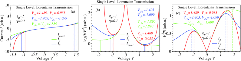 |
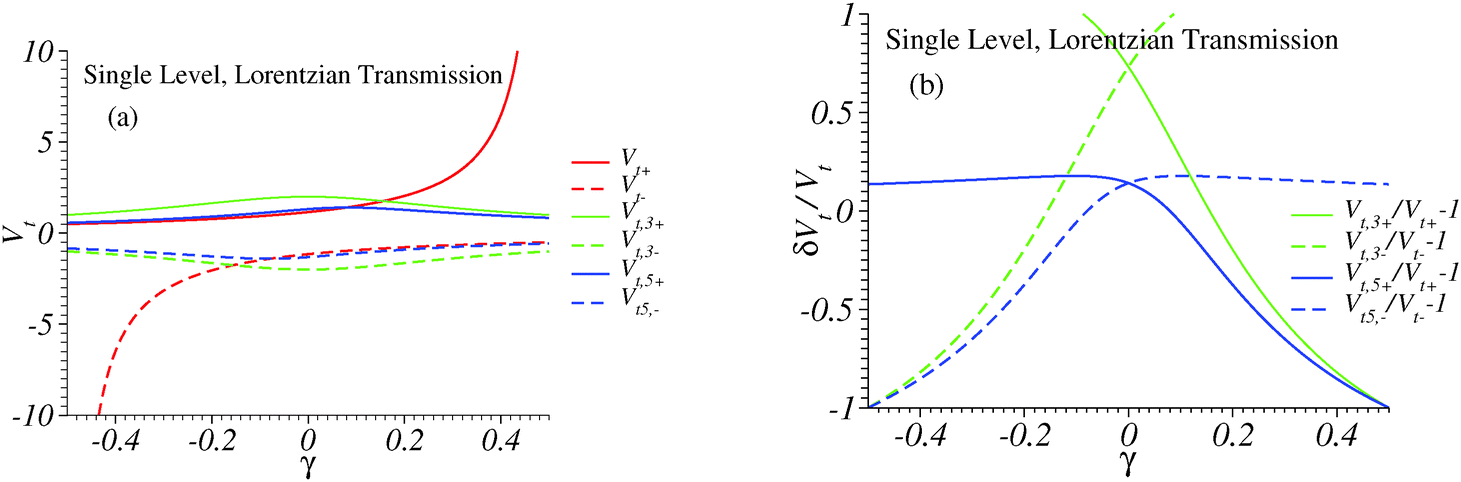
| | Fig. 9 Results for a single level and Lorentzian transmission. Whether computed exactly, using the third- or fifth-order expansions eqn (S10) (ESI†), (35) and (36), respectively I–V curves are asymmetric with respect to the origin for a nonvanishing voltage division factor γ (panel (a)). The transition voltages (minima of the Fowler–Nordheim quantity in panel (b)) computed exactly from eqn (S11) (ESI†) for opposite polarities are of different magnitudes (Vt+ ≠ |Vt−|). The fifth-order expansion correctly describes this inequality (Vt,5+ ≠ |Vt,5−|), while the third-order expansion incorrectly predicts Vt,3+ = |Vt,3−|. | |
Although calculations are straightforward, being too lengthy, the counterpart of the formulae given for symmetric I–V curves in the preceding section will not be given here. Instead, we will restrict ourselves to the Newns–Anderson (NA) model48–52 within the wide-band limit, which assumes a single level of energy εB(V) and Lorentzian transmission. For (off-resonant) situations of practical interest (Γ ≪ εB, biases up to ∼1.5εB/e),29,31,46,53–57 exact formulae for the current and Vt± have been deduced;12 see eqn (S10) and (S11) in the ESI.† The fifth-order expansion in eqn (S10) (ESI†) straightforwardly yields the expansion coefficients entering eqn (36)
| | ![[c with combining tilde]](https://www.rsc.org/images/entities/i_char_0063_0303.gif) 1 = −2γ; 2 = ¼ + 3γ2 1 = −2γ; 2 = ¼ + 3γ2 | (40) |
| |  | (41) |
where
j ≡
cj(
εB/
e)
j (
j = 1 to 4). By inserting the above expression into
eqn (37) and (38), the approximate values of
Vt,3± and
Vt,5± for both bias polarities can be obtained. The comparison with the exact
Vt± obtained from eqn (S11) (ESI
†) is depicted in Fig. S6 (ESI
†) and
Fig. 9 and 10.
 |
| | Fig. 10 Results for a single level and Lorentzian transmission. Transition voltages for positive and negative biases computed exactly Vt± from eqn (S11) (ESI†), and using the the third- or fifth-order expansions [Vt,3∓, eqn (35), and Vt,5±, eqn (36), respectively]. Note the incorrect prediction Vt,3+ = |Vt,3−|. The fifth-order expansion provides good estimates Vt,5± ≃ Vt± only for small γ; at larger γ, only one polarity is satisfactorily described (e.g., Vt,5− ≈ Vt− for γ > 0). | |
To end this subsection, lower order expansions (eqn (35) and (36)) for the asymmetric I–V curves considered above appear to be more problematic than for symmetric cases. Fig. 10 shows that even the fifth-order expansion provides a satisfactory description for both bias polarities only for weak asymmetries (|γ| ≲ 0.1).
6 Case of molecular junctions based on oligophenylene dithiols
Analytical expressions for current and conductance like those given above are very often utilized by experimentalists to fit their measurements. However, this is one important point on which the present work wants to emphasize that these formulae are only valid under well defined conditions/restrictions, and utilization beyond these conditions makes no sense. To exemplify, in this section we will analyze recent transport data obtained for molecular junctions based on oligophenylenes using silver electrodes Ag/OPD/Ag containing up to four phenyl rings (1 ≤ N ≤ 4).8
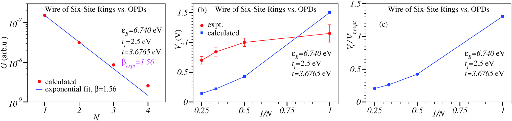
Experimental studies of OPD-based molecular junctions with silver electrodes containing 1 ≤ N ≤ 4 phenyl rings yielded a value of the conductance attenuation factor β ≃ 1.56 per ring;8 for a phenyl ring size d1 = 4.3 Å, this corresponds to ≃ 0.36 Å−1.8 This β-estimate can be invoked to immediately rule out the tunneling barrier picture underlying models (i) and (ii) discussed above as a valid framework to analyze the charge transport in these junctions. Out of the phenylene dithiol species studied in ref. 8, it is only the four-member species, d → d4 = 4d1, that satisfies the conditions of eqn (12), d = 6.24 > 4. In fact, as discussed in detail recently,18,25 the Simmons model in its original formulation1 does not account for the fact that, in molecular junctions, electron motion is laterally confined. When lateral constriction is incorporated into theory, the condition becomes more restrictive. Instead of eqn (12), one should apply eqn (18), which is invalidated even for N = 4.
The presently employed parameter εB represents an effective barrier height, which also embodies image effects. According to eqn (13) and (9), to “explain” a certain β-value adjusted to fit experimental data, both εB and the effective mass m* can empirically be “adjusted” to make theory “agree” with experiment. However, what cannot be “manipulated” in this way is the β-value itself. The restriction expressed by eqn (18) represents the mathematical condition for a valid description within the tunneling barrier model, and it cannot be modified whatever “appropriate” is the choice of εB and m*.
The argument based on the (too small) β-value also demonstrates that a description based on the superexchange limit of tunneling, which underlines model (iii),11 is impossible. For β = 1.56, eqn (20) yields th/εB = 0.458, which is not much smaller than unity, as required by eqn (22). Again, whatever “appropriate” the adjustment of the parameters εB and th, they cannot be chosen to satisfy the condition required by theory for a valid superexchange mechanism, because the experimental data “fix” the value of β and thence viaeqn (20) the ratio th/εB. So, one should go beyond the superexchange limit.
The most straightforward generalization is to use model (iv) for a chain with having one level per monomer, for which theory does not impose restrictions to the ratio between εB and th. Within a microscopic description based on model (iv), th represents the hopping integral coupling the two HOMOs of two adjacent benzene rings. It can be deduced from the difference between the ionization energies I1 and I2 of benzene and biphenyl: 2th = I1 − I2. Quantum chemical calculations based on refined ab initio methods, EOM-CCSD (equation-of-motion coupled clusters: singles and doubles), as implemented in CFOUR58 and OVGF (outer valence Green's functions)59–61 done using GAUSSIAN 09,62 allowed us to reliably determine I1 and I2. The values are I1 = 9.219 eV and 9.197 eV, and I2 = 8.217 eV and 8.204 eV, respectively. They allow us to compute the hopping integral needed for calculations based on model (iv): th = 0.501 eV and 0.497 eV, respectively. The agreement between these two th-values demonstrates the reliability of the ab initio estimates. The direct ab initio determination of εB (the relative alignment between the HOMO and electrodes' Fermi level) is an issue too difficult to be addressed here. It can be determined from the experimental value Vt|N=1 ≃ 1.15 V for Ag/OPD1/Ag.8,27 The equation  12 yields εB = 0.996 eV. Exact currents for the Hamiltonian of eqn (S1) (ESI†) can be computed numerically, and this allows us to obtain Vt for various N. The results based on model (iv) using this ab initio estimate th = 0.5 eV and adjusting εB to the value εB = 0.996 eV fixed by the experimental value Vt|N=1 ≃ 1.15 V8 are completely unacceptable; not even an exponential decay of the conductance with increasing size N can be obtained.
In view of this disagreement, we have attempted to keep only one of the above parameters (either th = 0.5 eV or εB = 0.996 eV) and to determine the other by fitting the experimental value β = 1.56.8 Fixing εB = 0.996 eV yields th = 0.387 eV, while fixing th = 0.5 eV yields a value εB = 1.288 eV. The results obtained in this way are depicted in Fig. S6 (ESI†) and Fig. 11, respectively, and they show that none of these empirical changes can make model (iv) to provide a satisfactory description. Differences between the cases of a flat potential and a linearly varying potential are insignificant (Fig. S6c and Fig. 11c); so, the lack of information of the real spatial potential profile across junctions cannot be advocated as a possible source of this disagreement.
 |
| | Fig. 11 Results for model (iv) using the ab initio value th = 0.5 eV and the value εB = 1.288 eV obtained by fitting the experimental conductance tunneling attenuation coefficient β = 1.56 (panel (a))8 The agreement between the calculated Vt-values (panel (b)) and the experimental values is poor. The spatial potential profile across these junctions do not notably affect Vt, as illustrated by the results obtained for constant and linearly varying potentials (panel (c)). The points (panels (b) and (c)) and error bars (panel (b)) represent experimental results for CP-AFM Ag/OPD/Ag junctions.8 | |
A description based on model (v), which considers the phenyl rings explicitly, represents the highest reasonable refinement of a tight-binding approach to charge transport in OPD junctions. To determine, ti, which within this model is a characteristic of a ring, we use the lowest singlet excitation energy Eexc; it can be expressed as Eexc = 2ti. Using aug-cc-pVDZ basis sets, we have determined Eexc from EOM-CCSD58 and SAC-CI (symmetry adapted cluster/configuration interaction)62 calculations; the values are Eexc = 5.154 eV and Eexc = 5.051 eV, respectively. They are in good agreement with the experimental values: 4.9 eV63,64 and 5.0 eV.65 So, we use the value ti = 2.5 eV, which also agrees with the overall description of the excitation spectrum of benzene as well as with polyacetylene data.66 To determine t, we use again the difference between the lowest ionization energies of benzene and biphenyl. (Note that the parameter t of model (v), which is the hopping integral between neighboring C sites belonging to adjacent phenyl rings (Fig. 2b), is different from the parameter th of model (iv), which is the hopping integral between HOMOs of adjacent phenyl rings (Fig. 2a).) To reproduce I1 − I2 ≃ 1 eV (see above), a value t = 3.677 eV is needed. The very fact that t = 3.677 eV is larger than ti = 2.5 eV is unphysical; the hopping integral t associated with a single C–C bond cannot be larger than the hopping integral ti associated with neighboring carbon atoms in an aromatic ring characterized by C–C distances shorter than a single C–C bond (Fig. 2b). It is a clear expression that parameters of tight-binding models (however refined they are) cannot be adjusted to satisfactorily oligophenylene molecules. This finding is in line with recent studies demonstrating limitations of tight-binding approaches to molecules of interest for molecular electronics.67
Using the ab initio values t = 3.677 eV and ti = 2.5 eV and adjusting εB to fit Vt|N=1 ≃ 1.15 V yields εB = 3.433 eV. This parameter set is not even able to qualitatively describe the exponential decay with N of the conductance. Therefore, we have also considered two alternative parameter sets: εB = 6.74 eV, ti = 2.5 eV, and t = 3.677 eV (Fig. 12) and εB = 3.433 eV, ti = 2.5 eV, and t = 0.964 eV (Fig. S7, ESI†). To obtain the first set, instead of fitting Vt|N=1 ≃ 1.15 V (as done above), we have adjusted εB by imposing β = 1.56. To obtain the second set, we have adjusted εB and t to fit the experimental values β = 1.56 and Vt|N=1 ≃ 1.15 V. Note that the value t = 0.964 eV is much smaller not only than the ab initio estimate t = 3.677 eV but also smaller than ti = 2.5 eV, which cannot be explained by the fact that a C–C single bond is slightly shorter than an aromatic one.68 As shown in Fig. 12 and Fig. S7 (ESI†), none of these two sets provide a satisfactory description.
 |
| | Fig. 12 Results for the conductance (panel (a)) and transition voltage (panels (b) and (c)) computed within model (v) using the values ti = 2.5 eV and t = 3.677 eV deduced ab initio and adjusting εB = 6.74 to fit the tunneling attenuation factor β = 1.56. In panel (b), the points and error bars represent experimental results for CP-AFM Ag/OPD/Ag junctions.8 | |
The (in)accuracy of Vt-estimates based on the third- and fifth-order expansions of eqn (1) and (4) using parameter values specific for OPD junctions, which is illustrated in Fig. S8 (ESI†), is comparable to that encountered in the previous situations (Fig. 3, 4 and 7, Fig. S1 and S5, ESI†).
To conclude this part, neither representing OPD junctions as chains of phenyl rings merely considering coupled HOMOs of neighboring rings within model (iv) nor a full treatment of the coupled rings at the tight binding level is able to provide an acceptable description of the transport experiments.8 Limitations of tight binding descriptions of molecules of interest for molecular electronics have been recently pointed out.67
The data collected in Table 1 demonstrate why a description based on a single level and Gaussian transmission should also be ruled out for OPD junctions. The difference between the values εB deduced from transport data8 and from ultraviolet photoelectron spectroscopy (UPS)27 for Ag/OPD1/Ag is enormous in the only case (N = 1) where the latter is available. In addition, εB, which represents the HOMO energy offset relative to the Fermi level, is found to increase with increasing N, which is completely unphysical.8
Table 1 Results obtained by modeling Ag/OPD/Ag by assuming a Gaussian transmission, eqn (S4) (ESI)
|
N
|
V
t
|
Δ
|
ε
B
|
ε
exptB
|
|
Experimental values.8
Results of ultraviolet photoelectron spectroscopy (UPS).27
|
| 1 |
1.15 |
1.273 |
3.061 |
1.1b |
| 2 |
1.00 |
1.265 |
3.378 |
|
| 3 |
0.84 |
1.212 |
3.615 |
|
| 4 |
0.70 |
1.118 |
3.639 |
|
7 Additional remarks
To avoid possible misunderstandings related to the present paper, a few remarks are in order, however. The above considerations refer to existing models, which are currently used for interpreting experimental data for charge transport via tunneling in molecular junctions. Our main aim was to present a list of formulae that can be used for data processing along with the pertaining applicability conditions. This paper is intended as a working instrument enabling to check whether certain experimental transport data are compatible or not with one of the existing models. By presenting the benchmark case of OPD-based junctions, we mainly aimed at illustrating how experimental data could/should be utilized to (in)validate a certain theoretical model, and not merely checking whether I–V measured curves can be fitted without checking whether the values of the fitting parameters are acceptable. An exhaustive analysis of transport data available in the literature for various molecular junctions within the presently considered models is beyond the present aim; this may make the object of a (review) paper of interest on its own.
The presently considered models disregard important physical effects (e.g., details of interface molecule–electrode couplings or metal-induced gap states). It may be entirely possible that none of these models are entirely satisfactory just because such effects are significant. The corresponding extension of the theoretical models to provide experimentalists with simple formulae enabling data processing/interpretation, obviating demanding microscopic transport calculations remains a desirable task for the future. In this paper we did not discuss the (off-resonant limit (Γ ≪ εB) of the) Newns–Anderson model in more detail. Relevant formulae (eqn (S10) and (S11)) are given in the ESI.† As shown in recent studies,8,69–71 cases where this description applies and is justified microscopically exist. There, the transition voltage can be used to directly extract the orbital energy offset using a formula ( for γ = 012) close to that initially claimed (eVt = εB).13 However, the results presented for the various models analyzed above have demonstrated that Vt cannot be uncritically used to straightforwardly deduce the energy alignment of the dominant molecular orbital. This does not diminish the importance of Vt. As emphasized in Section 2, Vt is an important property characterizing the nonlinear transport. By studying its behavior across homologous molecular classes (i.e., varying the molecular size d or n) or under gating (i.e., varying εB), the (in)applicability of a certain model can be concluded. Moreover, Vt turned out to be a key quantity, as it allowed us to reveal that charge transport across different experimental platforms and different molecular species exhibit a universal behavior, which can be even formulated as a law of corresponding states (LCS) free of any empirical parameters.71 In order to demonstrate that the cubic polynomial approximation is insufficiently accurate to describe Vt, we have presented in Fig. 1a a raw I–V trace measured on a CP-AFM junction.8 Making the point in connection with Fig. 1 is only possible by using neat, smooth curves; typical raw I–V curves measured for single-molecule junctions are blurry and therefore inadequate for this purpose. A comparison between junctions consisting of a single molecule and a bundle of molecules is of interest on its own; still, we note that, as long as the charge transfer occurs via off-resonant tunneling, the similarity between the transport properties of these two types of junctions is expressed by the aforementioned LCS.71 Considering transport through CP-AFM junctions within the models discussed above amounts to neglect proximity effects due to other (identical) molecules in the bundle. This assumption may certainly fail in some cases. However, the fact that OPD-based CP-AFM junctions obey this LCS71 can be taken as a strong indication that the failure of the various models in the case of these molecular devices discussed in Section 6 is not related to the approximate description in terms of a bundle of independent molecules.
8 Conclusion
With the manifest aim of providing experimental colleagues a comprehensive working framework enabling them to process and interpret measurements of transport by tunneling in molecular junctions, this paper have presented a detailed collection of analytical formulae, emphasizing on the fact (less discussed in the literature) that these formulae only hold if specific conditions of applicability are satisfied, which often impose severe restrictions on the model parameters. From a more general perspective, the theoretical results reported above have demonstrated that:
(i) The often accepted idea of a generic parabolic V-dependence of the conductance as a fingerprint of transport via tunneling emerged from studies based on high and wide energy barriers. This picture misses a microscopic foundation for tunneling across molecules characterized by discrete energy levels. At biases of experimental interest, within all the models examined here, the description based on a third-order expansion I = I(V) of transport measurements in molecular junctions is insufficient for quantitative purposes. To illustrate, we have shown this by systematically analyzing the fifth-order expansions, which turned out to be reasonably accurate at least for biases up to the transition voltages.
(ii) Merely adjusting model parameters (e.g., within a tunneling barrier picture by claiming renormalization effects due to image charges or effective mass) does not suffice to “make” a model valid for describing a specific molecular electronic device. On one side, models are normally valid only under specific conditions, which these parameters should satisfy. On the other side, the parameter values deduced from fitting experimental data should be consistent with ab initio estimates. Parameters for tight-binding models can be easily estimated via reliable ab initio quantum chemical calculations, as illustrated in this study.
(iii) The experimentally measured values of the β-tunneling coefficient of the low bias resistance can be inferred for quickly assessing the inapplicability of certain tunneling models. This turned out to be the case for OPD junctions, whose (too small) value (β = 1.56 or = 0.36 Å−1) deduced from experiment is incompatible with descriptions based on the tunneling barrier or superexchange mechanism. Because molecular junctions based on other aromatic aromatic species often have even smaller β's (β ≈ 0.2 Å−127,28), descriptions based on those models should be excluded. In such cases, the uncritical application of the mathematical formula of I vs. V is meaningless, even if the measured I–V curves can be satisfactorily fitted.
(iv) For biases not too much higher than the transition voltage, a realistic description of the spatial potential profile across a molecular junction appears to be considerably less important than that usually claimed. This is no longer the case at high biases, where the spatial potential profile may be responsible for qualitatively new phenomena, e.g., negative differential resistance (cf.Fig. 6).
(v) The fact that the estimate Vt,5 ≈ Vt based on the fifth-order I(V)-expansion turned out to be acceptable in many cases can be of practical help; eqn (4) (or eqn (36)) can be employed to process noisy experimental I–V curves, for which straightforwardly redrawing measurements as log(I/V2) vs. V (or V2/I vs. V) may yield substantial uncertainties to determine the minimum (or maximum) position. Fitting I–V curves with fifth-order polynomials can be used to extract the coefficients c2,3,4 and to estimate Vt ≈ Vt,5 by means of eqn (6) or (38).
(vi) Finally, we refer to situations where a successful description based on a single level and Lorentzian transmission (also known as the Newns–Anderson model) has been concluded.8,69,70 The fact that the I–V curves could be very well fitted within the Newns–Anderson framework was not the only argument leading to that conclusion; equally important was that the energy offset εB deducing from fitting the I–V data has been correlated with ab initio estimates8,70 and/or independent experimental information.69 Even if the transport would have been dominated by a single level, the conclusion of those studies would have not emerged in the case of, e.g. a Gaussian transmission, because of the completely different dependence of Vt on εB.
With the (few) examples mentioned in the preceding paragraph, we want to end by reiterating an idea already presented in Introduction: while attempting to make the community more aware of the limits of applicability of the various models utilized, the present paper did by no means intend to challenge the overall usefulness of model-based studies in gaining conceptual insights into the charge transport by tunneling at the nanoscale.
Acknowledgements
Financial support provided by the Deutsche Forschungsgemeinschaft (grant BA 1799/2-1) is gratefully acknowledged.
References
- J. G. Simmons, J. Appl. Phys., 1963, 34, 1793–1803 CrossRef
 .
.
- J. G. Simmons, J. Appl. Phys., 1963, 34, 238–239 CrossRef .
-
J. Rowell, Tunneling Phenomena in Solids, Springer, US, 1969, pp. 385–404 Search PubMed .
-
C. B. Duke, Tunneling Phenomena in Solids, Springer, US, 1969, ch. 28, pp. 31–46 Search PubMed .
-
C. B. Duke, Tunneling in Solids, Academic Press, NY, 1969 Search PubMed .
- W. F. Brinkman, R. C. Dynes and J. M. Rowell, J. Appl. Phys., 1970, 41, 1915–1921 CrossRef CAS .
-
J. C. Cuevas and E. Scheer, Molecular Electronics: An Introduction to Theory and Experiment, World Scientific Publishers, 2010 Search PubMed .
- The author thanks Dan Frisbie and Zuoti Xie for providing him the experimental data for CP-AFM Ag/OPDn/Ag junctions used in this work.
- A. Vilan, D. Cahen and E. Kraisler, ACS Nano, 2013, 7, 695–706 CrossRef CAS PubMed .
- In most part of this paper we restrict our analysis to I–V curves symmetric with respect to origin I(−V) = −I(V) and omit even powers in the current expansion, eqn (1) and (4), since this symmetry characterizes the OPD-based junctions,8 to which we pay a particular attention in this study.
- V. Mujica and M. A. Ratner, Chem. Phys., 2001, 264, 365–370 CrossRef CAS .
- I. Bâldea, Phys. Rev. B: Condens. Matter Mater. Phys., 2012, 85, 035442 CrossRef .
- J. M. Beebe, B. Kim, J. W. Gadzuk, C. D. Frisbie and J. G. Kushmerick, Phys. Rev. Lett., 2006, 97, 026801 CrossRef PubMed .
- The author thanks Dan Frisbie for stimulating him to propose this alternative graphical representation (“PVS”) to the Fowler–Nordheim plots used in earlier studies on transition voltage spectroscopy, because the latter may unphysically relate Vt to a mechanistic transition13 from a direct tunneling to a Fowler–Nordheim tunneling regime, which in fact does not occur at V = Vt. For this reason, the term “Peak Voltage Spectroscopy” (PVS) suggested by the plots depicted in Fig. S1c, S2c, S3c, S4c and S9c (ES†) may be more appropriate than “Transition Voltage Spectroscopy” (TVS).
- K. Gundlach and J. Simmons, Thin Solid Films, 1969, 4, 61–79 CrossRef CAS .
- A. Nitzan, Annu. Rev. Phys. Chem., 2001, 52, 681–750 CrossRef CAS PubMed .
- M. Araidai and M. Tsukada, Phys. Rev. B: Condens. Matter Mater. Phys., 2010, 81, 235114 CrossRef .
- I. Bâldea and H. Köppel, Phys. Lett. A, 2012, 376, 1472–1476 CrossRef .
- I. Bâldea, A. K. Gupta, L. S. Cederbaum and N. Moiseyev, Phys. Rev. B: Condens. Matter Mater. Phys., 2004, 69, 245311 CrossRef .
- E. H. Huisman, C. M. Guédon, B. J. van Wees and S. J. van der Molen, Nano Lett., 2009, 9, 3909–3913 CrossRef CAS PubMed .
- I. Bâldea, Chem. Phys., 2010, 377, 15–20 CrossRef .
- R. H. Fowler, Proc. R. Soc. London, Ser. A, 1928, 117, 549–552 CrossRef CAS .
- R. H. Fowler and L. Nordheim, Proc. R. Soc. London, Ser. A, 1928, 119, 173–181 CrossRef CAS .
- L. W. Nordheim, Proc. R. Soc. London, Ser. A, 1928, 121, 626–639 CrossRef .
- I. Bâldea, Europhys. Lett., 2012, 98, 17010 CrossRef .
-
R. Balescu, Equilibrium and Nonequilibrium Statistical Mechanics, John Wiley & Sons Inc., 1975 Search PubMed .
- B. Kim, S. H. Choi, X.-Y. Zhu and C. D. Frisbie, J. Am. Chem. Soc., 2011, 133, 19864–19877 CrossRef CAS PubMed .
- J. Balachandran, P. Reddy, B. D. Dunietz and V. Gavini, J. Phys. Chem. Lett., 2012, 3, 1962–1967 CrossRef CAS .
- I. Bâldea, J. Am. Chem. Soc., 2012, 134, 7958–7962 CrossRef PubMed .
- S. Guo, J. Hihath, I. Diez-Pérez and N. Tao, J. Am. Chem. Soc., 2011, 133, 19189–19197 CrossRef CAS PubMed .
- S. Guo, G. Zhou and N. Tao, Nano Lett., 2013, 13, 4326–4332 CrossRef CAS PubMed .
-
A. Sommerfeld and H. Bethe, Handbuch der Physik, Julius-Springer-Verlag, Berlin, 1933, vol. 24 (2), p. 446 Search PubMed .
- M. L. Trouwborst, C. A. Martin, R. H. M. Smit, C. M. Guédon, T. A. Baart, S. J. van der Molen and J. M. van Ruitenbeek, Nano Lett., 2011, 11, 614–617 CrossRef CAS PubMed .
- K. Sotthewes, C. Hellenthal, A. Kumar and H. Zandvliet, RSC Adv., 2014, 4, 32438–32442 RSC .
- I. Bâldea, RSC Adv., 2014, 4, 33257–33261 RSC .
- N. M. Miskovsky, P. H. Cutler, T. E. Feuchtwang and A. A. Lucas, Appl. Phys. A: Mater. Sci. Process., 1982, 27, 139–147 CrossRef .
- R. G. Forbes, J. Appl. Phys., 2008, 103, 114911 CrossRef .
- H. M. McConnell, J. Chem. Phys., 1961, 35, 508–515 CrossRef CAS .
-
H. J. W. Haug and A.-P. Jauho, Quantum Kinetics in Transport and Optics of Semiconductors, Springer Series in Solid-State Sciences, Berlin, Heidelberg, New York, 2nd edn, 2008, vol. 123 Search PubMed .
- A. Onipko and Y. Klymenko, J. Phys. Chem. A, 1998, 102, 4246–4255 CrossRef CAS .
- A. Cruz, A. Mishra and W. Schmickler, Electrochim. Acta, 2011, 56, 5245–5251 CrossRef CAS .
- R. Stratton, J. Phys. Chem. Solids, 1962, 23, 1177–1190 CrossRef .
- I. Bâldea and H. Köppel, Phys. Rev. B: Condens. Matter Mater. Phys., 2010, 81, 193401 CrossRef .
- I. V. Pobelov, Z. Li and T. Wandlowski, J. Am. Chem. Soc., 2008, 130, 16045–16054 CrossRef CAS PubMed .
- H. Song, Y. Kim, Y. H. Jang, H. Jeong, M. A. Reed and T. Lee, Nature, 2009, 462, 1039–1043 CrossRef CAS PubMed .
- W.-Y. Lo, W. Bi, L. Li, I. H. Jung and L. Yu, Nano Lett., 2015, 15, 958–962 CrossRef CAS PubMed .
- A. Tan, S. Sadat and P. Reddy, Appl. Phys. Lett., 2010, 96, 013110 CrossRef .
- D. M. Newns, Phys. Rev., 1969, 178, 1123–1135 CrossRef CAS .
- J. Muscat and D. Newns, Prog. Surf. Sci., 1978, 9, 1–43 CrossRef CAS .
- P. W. Anderson, Phys. Rev., 1961, 124, 41–53 CrossRef CAS .
- W. Schmickler, J. Electroanal. Chem., 1986, 204, 31–43 CrossRef CAS .
-
M.-C. Desjonqueres and D. Spanjaard, Concepts in Surface Physics, Springer Verlag, Berlin, Heidelberg, New York, 1996 Search PubMed .
- K. Smaali, N. Clément, G. Patriarche and D. Vuillaume, ACS Nano, 2012, 6, 4639–4647 CrossRef CAS PubMed .
- G. Ricoeur, S. Lenfant, D. Guérin and D. Vuillaume, J. Phys. Chem. C, 2012, 116, 20722–20730 Search PubMed .
- D. Fracasso, M. I. Muglali, M. Rohwerder, A. Terfort and R. C. Chiechi, J. Phys. Chem. C, 2013, 117, 11367–11376 CAS .
- K. Smaali, S. Desbief, G. Foti, T. Frederiksen, D. Sanchez-Portal, A. Arnau, J. P. Nys, P. Leclere, D. Vuillaume and N. Clement, Nanoscale, 2015, 7, 1809–1819 RSC .
- X. Lefèvre, F. Moggia, O. Segut, Y.-P. Lin, Y. Ksari, G. Delafosse, K. Smaali, D. Guérin, V. Derycke, D. Vuillaume, S. Lenfant, L. Patrone and B. Jousselme, J. Phys. Chem. C, 2015, 119, 5703–5713 Search PubMed .
- CFOUR, Coupled-Cluster techniques for Computational Chemistry, a quantum-chemical program package by J.F. Stanton, J. Gauss, M.E. Harding, P.G. Szalay with contributions from A.A. Auer, R.J. Bartlett, U. Benedikt, C. Berger, D.E. Bernholdt, Y.J. Bomble, L. Cheng, O. Christiansen, M. Heckert, O. Heun, C. Huber, T.-C. Jagau, D. Jonsson, J. Jusélius, K. Klein, W.J. Lauderdale, D.A. Matthews, T. Metzroth, L.A. Mück, D.P. O'Neill, D.R. Price, E. Prochnow, C. Puzzarini, K. Ruud, F. Schiffmann, W. Schwalbach, C. Simmons, S. Stopkowicz, A. Tajti, J. Vázquez, F. Wang, J.D. Watts and the integral packages MOLECULE (J. Almlöf and P. R. Taylor), PROPS (P. R. Taylor), ABACUS (T. Helgaker, H. J. Aa. Jensen, P. Jørgensen, and J. Olsen), and ECP routines by A. V. Mitin and C. van Wüllen. For the current version, see http://www.cfour.de.
- L. S. Cederbaum, J. Phys. B: At. Mol. Phys., 1975, 8, 290 CrossRef CAS .
-
L. S. Cederbaum and W. Domcke, Adv. Chem. Phys., Wiley, New York, 1977, vol. 36, pp. 205–344 Search PubMed .
- W. von Niessen, J. Schirmer and L. S. Cederbaum, Comput. Phys. Rep., 1984, 1, 57–125 CrossRef CAS .
-
M. J. Frisch, G. W. Trucks, H. B. Schlegel, G. E. Scuseria, M. A. Robb, J. R. Cheeseman, G. Scalmani, V. Barone, B. Mennucci, G. A. Petersson, H. Nakatsuji, M. Caricato, X. Li, H. P. Hratchian, A. F. Izmaylov, J. Bloino, G. Zheng, J. L. Sonnenberg, M. Hada, M. Ehara, K. Toyota, R. Fukuda, J. Hasegawa, M. Ishida, T. Nakajima, Y. Honda, O. Kitao, H. Nakai, T. Vreven, J. A. Montgomery Jr., J. E. Peralta, F. Ogliaro, M. Bearpark, J. J. Heyd, E. Brothers, K. N. Kudin, V. N. Staroverov, T. Keith, R. Kobayashi, J. Normand, K. Raghavachari, A. Rendell, J. C. Burant, S. S. Iyengar, J. Tomasi, M. Cossi, N. Rega, J. M. Millam, M. Klene, J. E. Knox, J. B. Cross, V. Bakken, C. Adamo, J. Jaramillo, R. Gomperts, R. E. Stratmann, O. Yazyev, A. J. Austin, R. Cammi, C. Pomelli, J. W. Ochterski, R. L. Martin, K. Morokuma, V. G. Zakrzewski, G. A. Voth, P. Salvador, J. J. Dannenberg, S. Dapprich, A. D. Daniels, O. Farkas, J. B. Foresman, J. V. Ortiz, J. Cioslowski and D. J. Fox, Gaussian 09, Revision B.01, Gaussian, Inc., Wallingford CT, 2010 Search PubMed .
- J. H. Callomon, T. M. Dunn and J. M. Mills, Philos. Trans. R. Soc., A, 1966, 259, 499–532 CrossRef CAS .
- E. N. Lassettre, A. Skerbele, M. A. Dillon and K. J. Ross, J. Chem. Phys., 1968, 48, 5066–5096 CrossRef CAS .
- J. P. Doering, J. Chem. Phys., 1969, 51, 2866–2870 CrossRef CAS .
- I. Bâldea and L. S. Cederbaum, Phys. Rev. B: Condens. Matter Mater. Phys., 2007, 75, 125323 CrossRef .
- I. Bâldea, Faraday Discuss., 2014, 174, 37–56 Search PubMed .
- W. P. Su, J. R. Schrieffer and A. J. Heeger, Phys. Rev. B: Condens. Matter Mater. Phys., 1980, 22, 2099–2111 CrossRef CAS .
- I. Bâldea, Nanoscale, 2013, 5, 9222–9230 RSC .
- I. Bâldea, Nanotechnology, 2014, 25, 455202 CrossRef PubMed .
- I. Bâldea, Z. Xie and C. D. Frisbie, Nanoscale, 2015, 7, 10465–10471 RSC .
Footnotes |
| † Electronic supplementary information (ESI) available. See DOI: 10.1039/c5cp02595h |
| ‡ Also at National Institute for Lasers, Plasmas, and Radiation Physics, Institute of Space Sciences, RO 077125, Bucharest-Măgurele, Romania. |
|
| This journal is © the Owner Societies 2015 |
Click here to see how this site uses Cookies. View our privacy policy here. 
 Open Access Article
 This Open Access Article is licensed under a

 is the low bias conductance.10


 stands for the junction's transverse area and
 , m0 and m* are Sommerfeld's constant,32 free and effective electron mass, respectively. Eqn (12) (like eqn (18) below) defines a dimensionless junction width z. The transition voltage for the Simmons and Simmons-based models has been investigated in a series of recent studies.18,20,25,33–35


 .12,21,29 In fact, both the proportionality to εB and the insensitivity to Γ-variations for Γ ≪ εB are common features shared by the above models (iii–v), while a Vt nearly proportional to εB1/2 at large εB for models (i) and (ii) is the consequence of the fact that the corresponding transmissions are similar to that of eqn (26) with δ = 1/2 (cf.eqn (17) and (30)). Common features for these two types of transmissions are the inflection point of the I–V curves (“current steps”, Fig. 8a) located at biases Vres = 2εB/e where the level becomes resonant to electrodes' Fermi energy, and the fact that the associated maximum in the differential conductance has a width proportional to the transmission widths; δVres ∝ Δ (Fig. 8b), similar to δVres ∝ Γ for Lorentzian transmission. The opposite dependence of Vt on εB for Lorentzian (Vt ∝ εB) and Gaussian (Vt ∝ 1/εB) transmission is relevant for the correctly interpreting gating effects44–46 or the impact of electrodes' work function.27


 for γ = 0