
 Open Access Article
 This Open Access Article is licensed under a
 Creative Commons Attribution 3.0 Unported Licence
Temperature-induced structural transitions in self-assembling magnetic nanocolloids
Sofia S.
Kantorovich
*ab,
Alexey O.
Ivanov
b,
Lorenzo
Rovigatti
a,
Jose M.
Tavares
cd and
Francesco
Sciortino
e
aUniversity of Vienna, Sensengasse 8, 1090, Vienna, Austria. E-mail: sofia.kantorovich@univie.ac.at
bUral Federal University, Lenin Av. 51, 620000, Ekaterinburg, Russia
cCentro de Física Teórica e Computacional da Universidade de Lisboa, Faculdade de Ciências, Campo Grande, 1749-016 Lisboa, Portugal
dInstituto Superior de Engenharia de Lisboa-ISEL, Rua Conselheiro Emídio Navarro 1, 1950-062 Lisboa, Portugal
eUniversity of Rome La Sapienza, Piazzale Aldo Moro 2, I-00185, Roma, Italy
First published on 29th May 2015
Abstract
With the help of a unique combination of density functional theory and computer simulations, we discover two possible scenarios, depending on concentration, for the hierarchical self-assembly of magnetic nanoparticles on cooling. We show that typically considered low temperature clusters, i.e. defect-free chains and rings, merge into more complex branched structures through only three types of defects: four-way X junctions, three-way Y junctions and two-way Z junctions. Our accurate calculations reveal the predominance of weakly magnetically responsive rings cross-linked by X defects at the lowest temperatures. We thus provide a strategy to fine-tune magnetic and thermodynamic responses of magnetic nanocolloids to be used in medical and microfluidics applications.
1 Introduction
The first stable suspensions of magnetic nanoparticles, nowadays known as ferrofluids,1,2 were synthesised more than 50 years ago.3 Since then, the design of magnetic colloids has steadily progressed: it is now possible to functionalise the nanoparticle surfaces,4,5 tune their shape6–12 and control their internal crystalline structure.13–15 Such a flexibility in design has opened broad perspectives for applications of magnetic nanocolloids in biomedicine, such as sensors, contrast agents, drug targeting, hypothermia cancer-treatment therapy, cell manipulation and many others;16–21 they also improved various technologies, such as loudspeakers, seals, dampers, purification and separation devices.22–24 Magnetic nanoparticles are attractive for all aforementioned applications because of their single-domain nature. Indeed, magnetic nanoparticles have intrinsic magnetic moments and behave as nanomagnets as long as their size does not exceed the size of a magnetic domain. The latter depends on the ferri- or ferromagnetic material the particle is made of, but it is usually in the range of 10–50 nm. Another important common property of all these magnetic nanocolloids is that, once in solution, they undergo brownian motion. Moreover, if the magnetic crystallographic anisotropy of a nanoparticle is energetically strong enough, then the orientation of the magnetic moment is coupled to the orientation of the particle as a rigid body,25 so that the two cannot rotate independently.Notwithstanding the way the surface of a magnetic nanoparticle is treated (be it special funtionalisation, steric or electrostatic stabilisation) there is an inevitable long-range, anisotropic dipolar interaction between nanoparticles' magnetic moments. This interaction introduces a preferred head-to-tail orientation of dipole moments and, if strong enough to compete with thermal fluctuations, leads to a directional self-assembly of particles in linear flexible chains.26–31 Of course, controlling self-assembly in magnetic nanocolloids is not restricted by magnetic forces only. Van der Waals, electrostatic or chemical interactions of functionalised particle surfaces, solvophilicity/solvophobicity of nanoparticle shells; all these and many others can result in versatile self-assembly scenarios.32–34 It is interesting to observe in this respect the analogies between the anisotropically interacting dipolar nanoparticles and patchy colloids with a reduced valence.35,36 Indeed, restricting the particle–particle relative orientations that result in a bond, leads to self-assembly processes that resemble the one occurring in dipolar nanoparticles, suggesting the possibility to extend the recent investigations of patchy colloids to dipolar fluids. For example, many novel and technologically-relevant phases, such as open lattices,37,38 equilibrium gels39,40 and reentrant gas–liquid phase separations,41,42 can be produced by a fine tuning of the patchy colloids parameters.
Along with an impressively rich spectrum of phases and structures induced by the aforementioned short-ranged or screened long-range interparticle interactions, magnetic nanocolloids, even if only magnetic forces are considered, experience a much more complex self-assembly scenario than that of linear chains: ring structures43,44 and networks of nanoparticles can form in these systems.45,46 Experimentally, these microstructures can be observed in solution using cryogenic electron microscopy47 and atomic force microscopy of assemblies at cross-linkable oil–water interfaces.48 On the numerical side, various simulation studies have been brought forward to describe self-assembly in magnetic nanocolloids by using simple models of dipolar hard- or soft-spheres.45,49,50 Recently, we showed that in highly diluted gas of dipolar hard spheres, chains turn into rings as temperature decreases.51 This structural transition provided a possible solution to a long-lasting debate about the non-monotonic temperature dependence of initial magnetic susceptibility in the suspensions of magnetic nanoparticles.52,53 However, at higher concentrations of magnetic nanoparticles, the assumption of non-interacting chains and rings is not valid any more, and one needs to take into account the next hierarchical step: self-assembly of chains and rings (in the following referred to as primary structures) into more complex branched structures and, eventually, into networks. One of the first attempts to handle branched structures in dipolar hard-sphere systems was introduced in ref. 54, 55, where a transition from pure chains to a system of branching chains (the gas of Y-junctions) was predicted. Even though Y-junctions are clearly one of the main branching mechanisms in dipolar hard spheres, their importance and abundance decrease dramatically with temperature.56
To shed light on the scenario of temperature-induced structural transitions in magnetic nanocolloids at moderate concentrations, we develop a theoretical approach and perform extensive Monte Carlo simulations, the result of which we present herein. Our theoretical approach is based on density-functional theory, where single nanoparticles can self-assemble in “defect-free” chains and rings as well as in “defect structures”, in which primary structures are merged with the help of specific “defect particles”. All these basic units are presented in Fig. 1. After a thorough numerical and visual analysis of simulation results,56 we identify three (and only three) defect particles, labeled in this paper as Y, X and Z defects. Defects Y include Safran's branching.54 The defects of types X and Y (see, Fig. 1) act as cross-linkers between primary structures. Defects of type Z do not link primary structures, rather they can be considered as internal defects of isolated chains and rings.
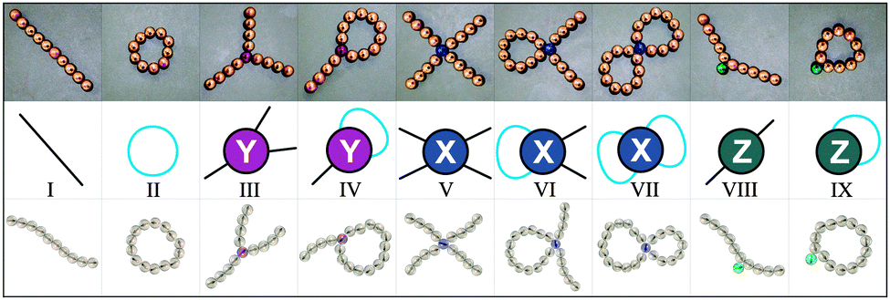 | ||
| Fig. 1 An overview of all the basic units we consider in three different representations. Top row: photographs of commercially available magnetic beads; middle row: topological classification used in the proposed theoretical approach, here in black we indicate chain segments and in blue – rings; bottom row: structures extracted from Monte Carlo computer simulations analysed in this paper. From left to right: (I) a linear chain of regular particles; (II) a ring of regular particles; (III) three linear chains of regular particles connected by one Y defect; (IV) one linear chain and one ring of regular particles connected by a Y defect; (V) four linear chains of regular particles connected by one X defect; (VI) one X defect connecting one ring and two chains of regular particles; (VII) one X defect joining two rings of regular particles; (VIII) a linear chain with an internal Z defect; (IX) a ring with an internal Z defect. | ||
In this paper we limit our theoretical analysis to the clusters that contain at most one defect. Even though our approach can in principle be extended to multiple defects, it is essential to understand the first steps of the hierarchical self-assembly of dipolar nanoparticles, namely the aggregation of single particles into primary structures and the subsequent merging of the latter into single-defect clusters. Focusing on the different defect types, we observe a clear hierarchy in the structures formed on cooling: first, when the thermal fluctuations are still comparable to the dipolar interactions, only short linear chains form. Then, when the thermal energy becomes smaller, depending on the concentration, two different sequences of structural transitions take place: mostly chains and rings form in the dilute regime, while chains, rings and branches appear in denser systems. Finally, at very high dipolar strength (or, conversely, at very low temperature) most of the Y defects are replaced by more energetically advantageous and infinitesimally magnetoresponsive defect structures made of two rings cross-linked by one X defect. Fig. 2 provides a cartoon of these different aggregation pathways.
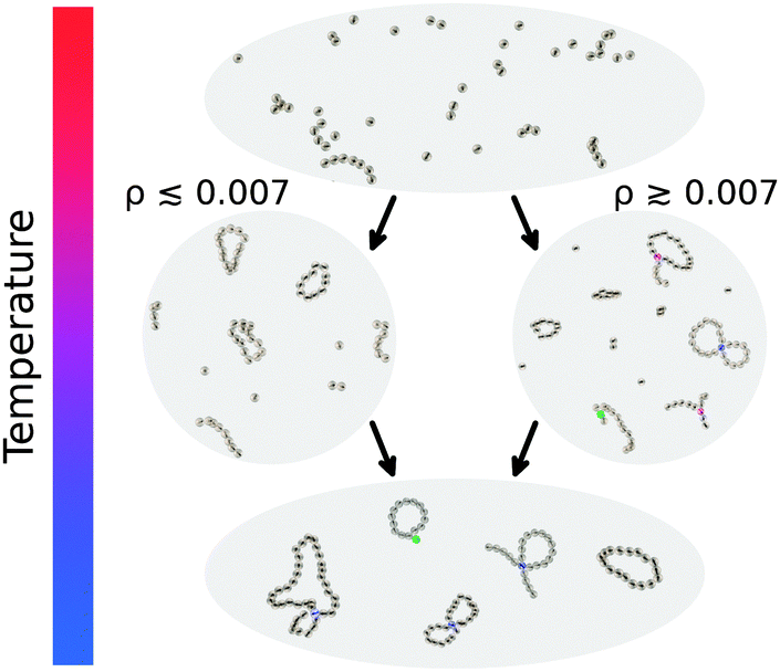 | ||
| Fig. 2 Cartoon sketching the temperature-induced structural transitions we observe at intermediate concentrations. | ||
2 Model and methods
2.1 Model
We investigate systems composed of N magnetic nanoparticles at varying temperature T and concentration c. Two particles i and j interact through the potential Vtot = VHS + Vdd, where VHS is the hard-sphere potential given by | (1) |
![[r with combining right harpoon above (vector)]](https://www.rsc.org/images/entities/i_char_0072_20d1.gif) ij| is the inter-particle distance and d is the particle diameter. Vdd is the dipole–dipole interaction, defined as follows:
ij| is the inter-particle distance and d is the particle diameter. Vdd is the dipole–dipole interaction, defined as follows: | (2) |
![[small mu, Greek, vector]](https://www.rsc.org/images/entities/i_char_e0e9.gif) k is the magnetic moment of particle k;
k is the magnetic moment of particle k;  . All the particle magnetic moments have the same magnitude μ.
In the text, kB is the Boltzmann constant, β = 1/T, lengths is measured in units of the particle diameter d and energy in units of μ2/d3. Therefore, temperature is measured in units of kBd3/μ2.
2.2 Theoretical approach
Our detailed analysis of branching in ref. 56 revealed the possibility to split all possible branching points in the system into three main classes only (see Fig. 1), using the number of ways out w (in the following “valency”) as a label. Looking at Fig. 1 one can see that particles of type Z have w = 2, particles of type Y are characterised by w = 3 and particles of type X have w = 4. Each of these defect particles also has a “charge” due to the possible dipolar orientations of defect neighbours: Y ones have charge 1 or −1, since if two dipoles enter the Y particle, then one necessarily exits (charge −1); conversely, if two dipoles exit, one enters (charge +1). By contrast, the charge of Z and X particles is always zero, since if one or two dipoles enter, one or two others always exit from the defect particle.In our model, defect particles do not interact with each other; rather they interact with “regular” particles. The latter can form chains and rings and as such connect defect particles. One can also think of our system as being composed by four different types of particles: one type can only form chains and rings, the other type (Z) can attach to a ring or to a chain, but cannot connect any of the two to some other cluster, whereas the other two (Y and X) connect chains and rings, effectively serving as cross-linkers with a fixed valency.
In Fig. 1 we showed the nine classes of structures that contain up to one defect particle. The free energy (F) per unit volume of this system can be obtained by summing up the free energies of these classes. In the following, we denote their equilibrium concentrations as g(·).
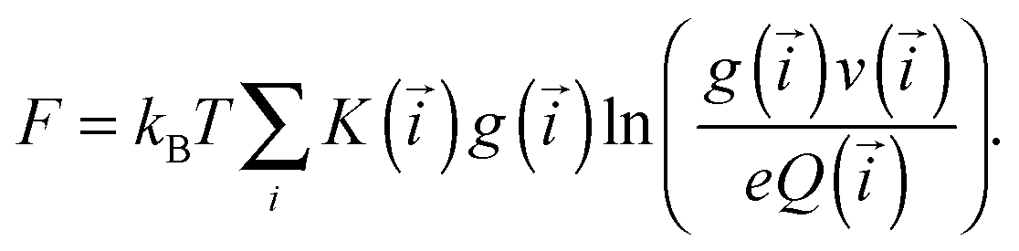 | (3) |
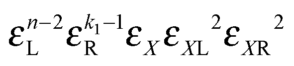
![[i with combining right harpoon above (vector)]](https://www.rsc.org/images/entities/i_char_0069_20d1.gif) containing the information about not only the size of the cluster but also about its topology, i.e.
containing the information about not only the size of the cluster but also about its topology, i.e.| = (n, k1, k2, mY, mX, mz) |
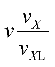
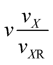
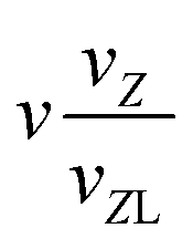
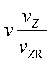
 for primary structures and 1 for the branches). In addition, the partition function of each class also depends on : Q(). Finally, v() is a characteristic volume, which allows us to express the partition functions in a simple factorised way (see, Table 1). The parameter K() is a combinatorial factor, representing the number of entropically distinguishable clusters from the same class, having the same and with the same partition function Q(). The free energy can thus be computed by minimising the functional (3) taking into account the mass-balance condition:
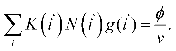 | (4) |
| Class |
|
v() |
N() |
Q() |
K() |
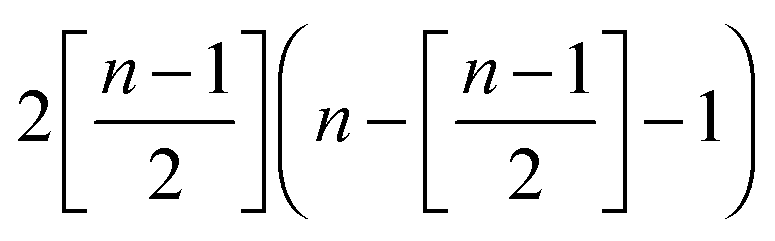
|---|---|---|---|---|---|
| a Here, the factor 2 reflects the possibility of Y defect to have a charge 1 or −1; [·] means the integer part of the argument. | |||||
| I | (n,0,0,0,0,0) | v | n |
|
1 |
| II | (0,k1,0,0,0,0) | v | k 1 |
|
1 |
| III | (n,0,0,1,0,0) |
|
n + 1 |
|
|
| IV | (n,k1,0,1,0,0) |

|
n + k1 + 1 |
|
2(k1 + 1)a |
| V | (n,0,0,0,1,0) |
|
n + 1 |
|
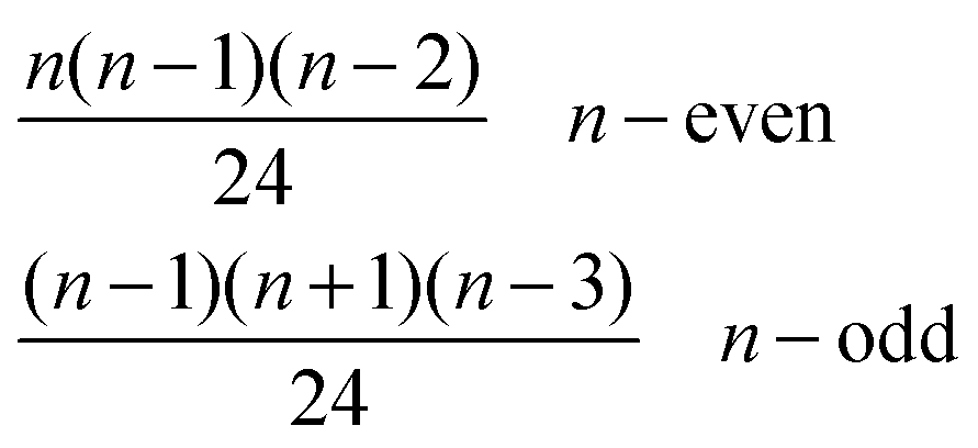
|
| VI | (n,k1,0,0,1,0) |

|
n + k1 + 1 |
|
(n − 1)(k1 + 1) |
| VII | (0,k1,k2,0,1,0) |
|
k 1 + k2 + 1 |
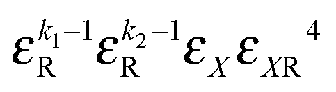
|
k 1 + k2 + 1 |
| VIII | (n,0,0,0,0,1) |
|
n + 1 |
|
n − 1 |
| IX | (0,k1,0,0,0,1) |
|
k 1 + 1 |
|
k 1 + 1 |
This condition constraints the total number of particles in a unit volume (ϕ/v, ϕ being regular particle volume fraction, v standing for particle volume). Note that the total number of regular particles in a cluster of class i is given by N(i) = n + k1 + k2 + mYsY + mXsX + mZsZ, where a defect particle depending on its type contains sY, sX or sZ regular particles. These parameters are used to simplify the description of the cluster formation. As shown in ref. 56, the number of particles in the defects can vary from one to four, however, the actual internal structure is irrelevant. Thus, we can unify the treatment and limit the number of defect particle types.
Minimisation using Lagrange multipliers method leads to a solution with a “traditional” functional form:
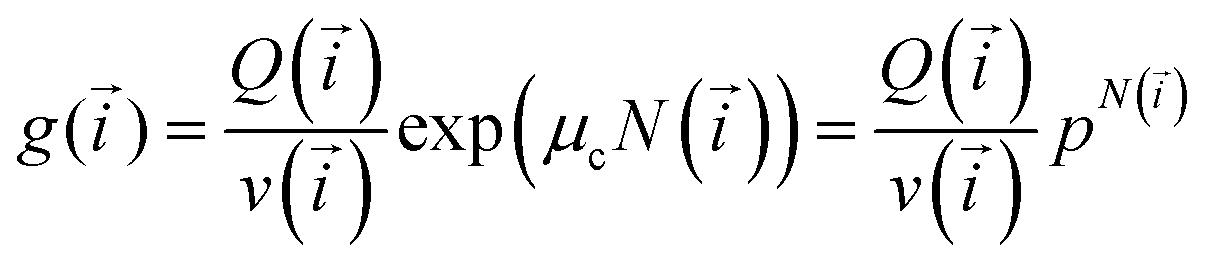 | (5) |
The main complexity of the problem is condensed in the analytical calculation of Q(), due to the long-range magnetic dipole–dipole interactions between nanoparticle magnetic moments. Here, we put forward an approach that makes use of the following assumptions:
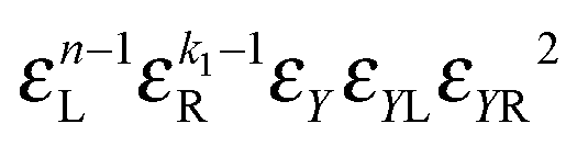
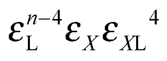
• Each bond is described by an effective free energy: εL for a linear chain segment, εR for a ring segment; εYL(YR) for a bond between the member of a chain (ring) segment and a defect particle Y; εXL(XR) for a bond between the member of a chain (ring) segment and a defect particle X; εZL(ZR) for a bond between the member of a chain (ring) segment and a defect particle Z; εl, l = X, Y, Z is the free energy loss of forming a defect l compared to a bond between regular particles.
• The partition function Q() can be factorised as a product of the aforementioned effective bond free energies and thus be computed as a function of the number of monomers and temperature, for details see ref. 51;
• The factorisation of Q() has a peculiarity, namely, even though it is presented as a product of effective free energies, these free energies actually do depend on the lengths of corresponding segments; in this way we can consider the interactions beyond the limit of the nearest neighbours;
• Entropic contributions are calculated with respect to the entropy of a chain, which is why the factor 1/k3v+1 is included in partition functions of ring containing clusters to capture the difference in entropy between chains and rings arising from the k ways of opening a ring to form a chain, where v = 0.588 is the self-avoiding random walk exponent; the difference number of self-avoiding paths of chains and rings is proportional to k3v.57
Building upon past results,51 we know that the bonding free energies associated to rings and chains are respectively given by
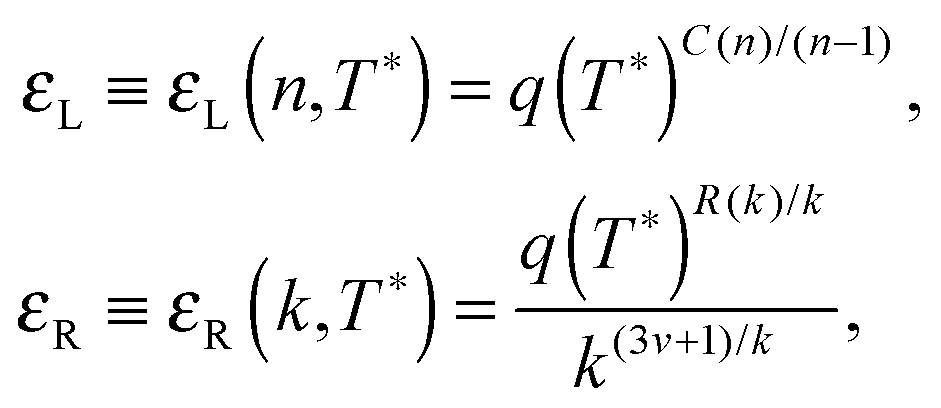 | (6) |
 | (7) |
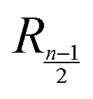 stands for the residual of division, and [·] has the meaning of the integer part of the expression in the brackets. The low-T dimer partition function q (note that C(1) = 0, C(2) = 1), derived first by de Gennes and Pincus,58 is
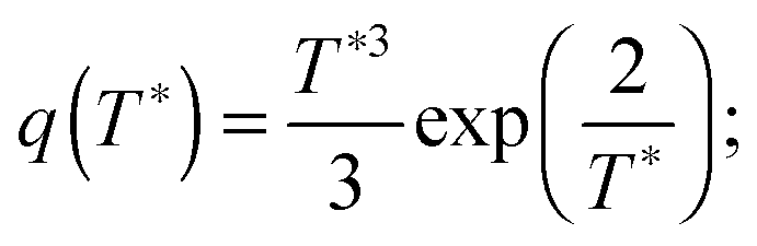 | (8) |
) = vY; analogously, for i = V, VI, VII the normalising volume is v() = vX and for i = VIII, IX we set v() = vZ. In addition, we introduce three parameters:| y = εYv/ṽY; x = εXv/ṽX; z = εZv/ṽZ. |
In the general case x, y, z are slowly changing functions of T*, and from previous investigations56 we know that x < y < z ≪ 1 for any temperature. Here, however, we neglect their temperature dependence and fit their values by matching the internal energy in simulations and theory, obtaining x = 0.003, y = 0.005 and z = 0.006. We performed an extensive analysis changing the values of these parameters by up to 60 per cent and discovered, that the microscopic characteristics as well as the thermodynamic quantities are not sensitive to such variations of x, y and z.
For the sake of simplicity, we fix sX = sZ = sY = 1. To justify the latter, we have carefully checked simulation results, finding that the amount of particles in defects is very small in comparison to the number of particles in ring and chain segments. We provide the expression for all the terms in the free energy functional (3) under these assumptions in Table 1.
Using this table, one can minimise the free energy of the system and obtain the Lagrange multiplier p as a function of temperature and nanoparticle concentration.
It is worth noting that, using the approach described above, we can introduce more complicated structures, that can be hierarchically obtained by combining the basic nine elements, as shown in Fig. 3. One can keep adding up defects following this approach to eventually build a percolating network of branched structures. The table can be relatively easily extended for this case, however, the calculation of the K values becomes more cumbersome. In any case, before dealing with the network itself it is crucially important to understand how the initial stage of branching occurs, which structures are more probable at low temperatures and what are the main tendencies in branching for different particle concentrations. In other words, we aim at understanding the second step (the first being the formation of primary structures, namely chains and rings) of the hierarchical self-assembly, thus elucidating the thermodynamics of the aggregation of primarily formed chains and rings into small branched clusters.
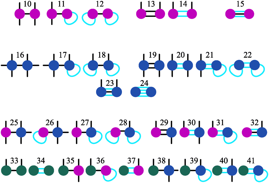 | ||
| Fig. 3 All possible 32 classes (from 10 to 41) of aggregates containing two defect particle. Defects Y are magenta, defects X are blue, defects Z are green, linear segments are black, ring segments are cyan. | ||
2.3 Computer simulations
We carry out Monte Carlo simulations in the canonical ensemble of N = 5000 dipolar hard spheres at different temperatures and concentrations φ = N/V ≪ 1, where V is the volume of the simulation box. We simulate down to T* = 0.125 by implementing ad-hoc biased Monte Carlo moves.44,59 For further details on the simulation approach, see ref. 44. We partition particles into clusters by employing a mixed distance/energy criterion: two particles are bonded if their pair-interaction energy is negative and their relative distance is smaller than rb = 1.3,44 which corresponds to the first minimum of the radial distribution function. Clusters are then classified according to these definitions:• a structure containing two single-bonded particles connected by particles having two neighbours is labelled as a chain;
• a ring is a cluster containing only particles having two neighbours;
• any other kind of aggregate is a branched cluster.
3 Results and discussion
The main advantage of the combined approach proposed here is that we can not only scrutinise the topologies of self-assembled magnetic nanoparticle clusters and their distributions at various concentrations and temperatures, but we can also directly follow the hierarchical self-assembly in these systems and estimate the thermodynamic contribution of each cluster type. In order to obtain a clear understanding of the concentration and temperature influence on the self-assembly in magnetic nanocolloids it is convenient to look at the fractions of particles in various clusters. In the following, we use dimensionless units for temperature (T*) and nanoparticle concentration (ρ*), as defined in Model and methods.3.1 Structural transitions
Fig. 4 shows the fraction of particles which are part of chains, rings or branched clusters. At high temperature, when the thermal fluctuations are strong enough to compete with magnetic dipole–dipole interparticle interactions, the majority of nanoparticles are connected in chains of various lengths.† If the concentration of nanoparticles is small and the temperature decreases, the chains increase in length and eventually the energetic gain of closing into rings becomes large enough for a structural transition to occur (Fig. 4 upper left). Further cooling the system drives the formation of more complex structures, even though their fraction never exceeds that of rings. A different scenario takes place at large nanoparticle concentration. In this case (Fig. 4 upper right, lower left and right), the environment becomes too crowded for ideal rings to dominate on cooling, and defect structures become increasingly relevant. The temperature of this structural transition grows slowly with growing nanoparticle concentration. We stress that our assumption that clusters can contain up to one defect is valid in a rather broad range of concentrations, as demonstrated by the good agreement between theoretical predictions and simulation results. However, for the highest concentration considered here (Fig. 4 lower right), the one-defect limitation becomes too strong since multiple-defect structures start to appear and the agreement between theoretical and numerical results degrades. It means that the structures considered here are the precursors to the next hierarchical level of self-assembly in magnetic nanocolloids, namely the aggregation of single-defect clusters into complex networks.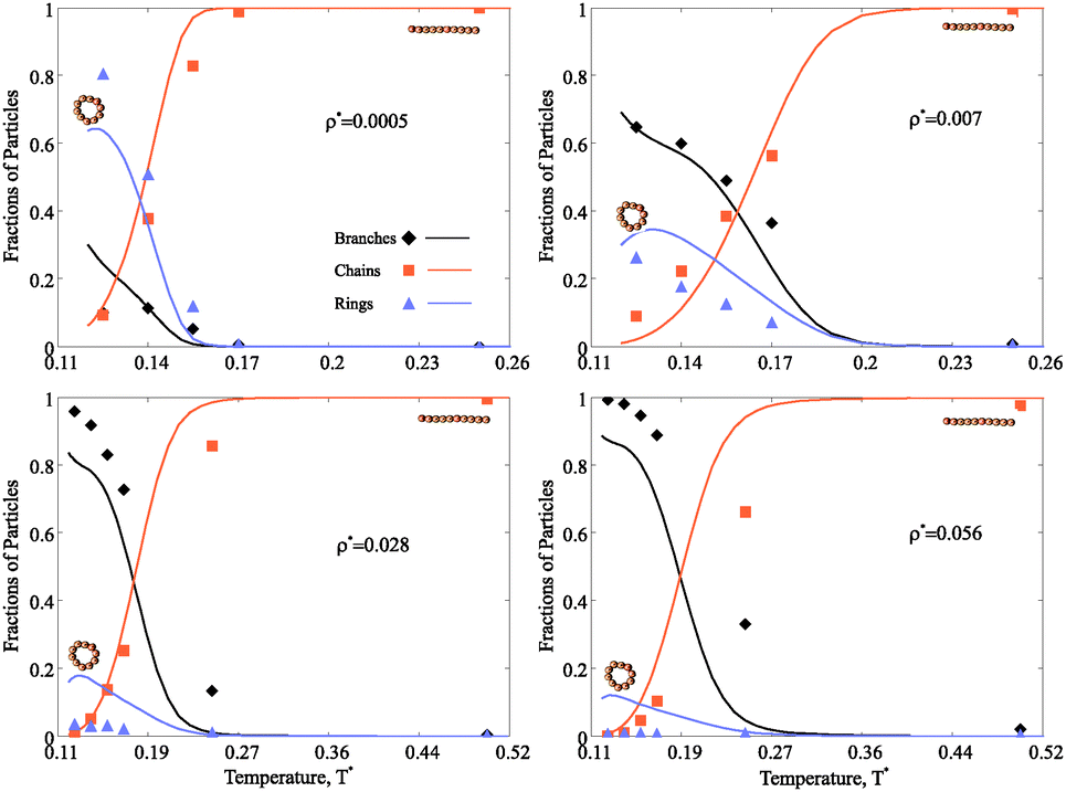 | ||
| Fig. 4 Fractions of chains, rings and defect structures for systems with different nanoparticle concentrations (ρ*) versus the dimensionless temperature (T*). The concentration grows from the left to the right and from the top to the bottom. In all four plots the same notations are used: solid lines are theoretical predictions, symbols denote the results of Monte Carlo Simulations. Simulation data for the fraction of chains is plotted with squares; for that of rings we use triangles; the fraction of all possible defect structures we visualise with rhombuses. When ρ* = 0.0005, at high T* the only clusters are chains, on cooling these chains close in rings; the fraction of nanoparticles in defect structures is very low even at very low temperature. For higher values of ρ*, the order of structural transitions is different, and the defect-free chains are replaced by defect structures on cooling. For ρ* = 0.056 the fraction of defect-free rings is basically negligible. | ||
3.2 Cluster distribution
Once it is clear that the high-T defect-free clusters are replaced by more complex structures upon cooling, the composition of these defect structures becomes of primary importance. Our theoretical approach allows us to scrutinise all possible transitions in detail. In order to illustrate the competition between different defect types, we show the temperature and concentration dependence of the fractions of particles in the various clusters in Fig. 5.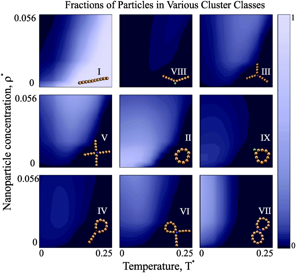 | ||
| Fig. 5 Class struggle: colour maps for the fraction of particles in various cluster classes as functions of dimensionless nanoparticle concentration and temperature. The colour-code is the same for each plot and is provided on the right: the brighter the colour is, the higher the fraction. The classes shown along the main diagonal (I, II, VII) do not exhibit any maxima in the range of studied parameters, whereas all the other structures have high fractions in well-defined T* − ρ* regions. In this figure one can clearly follow the hierarchical nature of the self-assembly in the systems under study. For example, the intracluster defects (VIII, IX) start to emerge with decreasing T*, but then quickly get replaced by more complex aggregates (III, IV, V, VI). Note that all these transitions are caused by the magnetic dipole–dipole interaction and entropy competition, which becomes more and more intricate. | ||
At high temperature, the overwhelming majority of particles is aggregated in chains, regardless of the concentration. As soon as the temperature decreases and the concentration grows, the first defect structures appear: chains begin to develop internal defects. As the system is further cooled down, Y structures first start to emerge and then slowly disappear in favour of X-structures. At the same time, rings with internal defects and tennis-racket-like structures (IV) are clearly overtaken by rings with two chain tails. If we cool the system further down, basically all defect-cluster fractions exhibit a clear maximum and start rapidly decreasing. For low concentrations, the majority of magnetic nanoparticles is aggregated in rings. For higher concentrations, though, the fraction of particles in rings has a maximum, signalling a transition towards the formation of higher-order defect clusters such as those in the VII class, i.e. double rings. These double rings thus form at temperatures lower than single rings, but at relatively high nanoparticle concentration they clearly become the dominant class. Another interesting aspect shown by Fig. 5 is that the fractions of chain-only defects decrease faster on cooling than those with at least one ring segment. This is a clear reminiscence of the low-concentration structural transitions on cooling, where the complete redistribution from chains into rings is observed in the same temperature range.51
3.3 Thermodynamics
Next we investigate the effect of the observed structural transitions on the thermodynamics of the magnetic nanoparticle systems. We start by considering how temperature and particle concentration affect the internal energy per particle, shown in Fig. 6.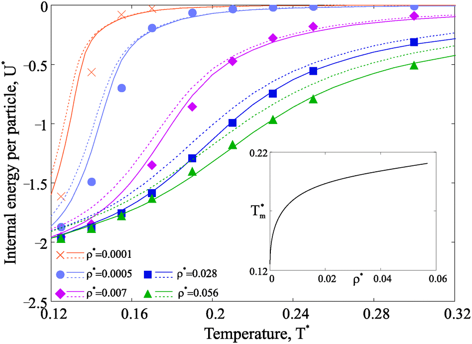 | ||
| Fig. 6 Internal energy U* as a function of T*. Simulation results for various concentrations are provided in symbols (see, legend). Theoretical solid lines agree well with simulation results, whereas the dashed curves, which show the internal energy of the system in which only chains can form, strongly deviate. The internal energy has a prefactor, which is set to unity in this plot: vd3/μ2V, where v and V are the volumes of the particle and the system respectively, μ is the value of the nanoparticle (diameter d) dipole moment. In the inset the temperature of the specific heat maxima Tm, i.e. the positions of the internal energy inflection points, is plotted as a function of the nanoparticle concentration. | ||
Several conclusions can be drawn when looking at Fig. 6. At any concentration the internal energy has an inflection point, which generates a maximum in the T dependence of the constant volume specific heat CV.60 The position of the maximum in CV, as shown in the inset, shifts towards low temperatures as the concentration decreases. Independently from concentration, there is only one specific heat maximum, whose position is in close correlation with the temperature of the first structural transition, be that chain-ring or chain-defect transition (compare to Fig. 4).
Taking advantage of the theoretical approach, one can compute the free energy and estimate its change across the various structural transitions. First we estimate the thermodynamic driving force which leads to the ring formation by calculating the free energy difference between a system composed by only chains and a system with chains and rings. At low concentrations, the possibility of forming rings drives to a dramatic decrease of the free energy and the contribution of rings to the system free energy becomes dominant at low temperature. These results are plotted with dashed lines in Fig. 7. For denser systems, though, the free energy gain due to ring formation is marginal. As a second step, we consider the free energy difference between a system composed only by chains and rings and a system composed of chains, rings and defects. The resulting driving force for branching is plotted with solid lines in the same figure (Fig. 7). The results show that, indeed, there is a significant driving force for branching, but only at intermediate and high densities in the studied range of temperature. This result confirms that the loss in the translational entropy of primary clusters on branching becomes less-and-less relevant with increasing density in comparison to the energetic contribution of the additional interaction.
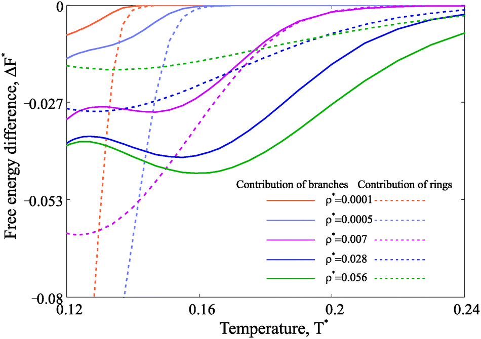 | ||
| Fig. 7 Free energy difference in units of T* calculated per particle. Dashed lines describe the free energy gain due to the ring formation in the model system with chains and rings only.51 The free energy gain obtained through the formation of branched structures (within the framework of the model proposed here) is plotted with solid lines. The legend for different nanoparticle concentrations is provided. | ||
4 Conclusions
In order to control the self-assembly of magnetic nanoparticles, one needs to gain a fundamental understanding of the interparticle interaction. Here, we reveal two scenarios of hierarchical self-assembly induced by cooling. Magnetic dipole–dipole interactions leads to the formation of non-bulky low-density structures in which the head-to-tail or antiparallel orientations of the dipoles are favourable. This can be realised by forming chains, rings, or various branches. The interplay between energy gains and entropy losses determines the internal structure of the self-assembling system and, as such, drastically influences the macroscopic responses of the systems. Even though nanoparticle rings have lower energy, at moderate temperatures, linear chains are predominant owing to their higher entropy. This changes on cooling. As a result, when the system of magnetic nanoparticles is highly diluted, the rings with a vanishing dipole moment turn out to be dominant. The same happens to the Y-type junctions, which form in the systems at higher nanoparticle concentration. However, the entropy gain of forming a Y-junction does not compensate for the energy decrease gained from the ring formation, thus making the structural behaviour of highly magnetic nanocolloids much more complex than expected. In this work, using a combined novel analytical-numerical approach, we discover a series of fascinating structural transitions. Indeed, we find that the system of magnetic nanocolloids exhibits two different scenarios of the hierarchical self-assembly. At low particle concentrations, first highly magnetically responsive linear chains are formed, which further close in rings, thus making the whole system barely susceptible to an external magnetic field. The weak interaction between nanoparticle rings increases on cooling, which leads to the formation of a particular type of defects, playing the role of ring cross linkers. In contrast, at higher nanoparticle concentration, at moderate temperature, chains are replaced by entropy-induced branched structures, which can be described by only three types of defects, X, Y and Z, classified according to the number of linear segments connected by the defect. On cooling Y and Z defects disappear, and the X-type defects dominate, merging together nanoparticle rings, keeping the system weakly magnetically responsive. The defect structures observed here can be considered as the precursors to the network formation, ushering in the next step of the hierarchical self-assembly of magnetic nanocolloids. Our theoretical frame-work developed here, combined with the approach put forward in ref. 54 can serve as a starting point to the description of the network formation.Acknowledgements
The research has been partially supported by Austrian Research Fund (FWF): START-Projekt Y 627-N27. L.R. acknowledges support from the Austrian Research Fund (FWF) through his Lise-Meitner Fellowship M 1650-N27. J.M.T. acknowledges financial support from the Portuguese Foundation for Science and Technology under Contracts No. EXCL/FISNAN/ 0083/2012 and UID/FIS/00618/2013. A.O.I. and S.S.K. are supported by the Ministry of Education and Science of the Russian Federation (Contract 02.A03.21.000, Project 3.12.2014/K). We are grateful to Michaela McCaffrey for taking pictures of magnetic balls used in the paper, and to Marcello Sega for fruitful discussions. F.S. and S.S.K. are grateful to the EU-Project: ETN-Colldense.References
- R. E. Rosensweig, Ferrohydrodynamics, Cambridge Univ. Press, Cambridge, 1985 Search PubMed.
- S. Odenbach and S. Thurm, Ferrofluids: Magnetically Controllable Fluids and Their Applications, Springer, Berlin, Germany, 2002, vol. 594, pp. 185–201 Search PubMed.
- L. Resler Jr and R. E. Rosensweig, AIAA J., 1964, 2, 1418–1422 CrossRef.
- S. K. Smoukov, S. Gangwal, M. Marquez and O. D. Velev, Soft Matter, 2009, 5, 1285–1292 RSC.
- S.-H. Kim, J. Sim, J.-M. Lim and S.-M. Yang, Angew. Chem., Int. Ed., 2010, 49, 3786–3790 CrossRef CAS PubMed.
- P. Tierno, Phys. Chem. Chem. Phys., 2014, 16, 23515–23528 RSC.
- M. Yan, J. Fresnais and J.-F. Berret, Soft Matter, 2010, 6, 1997–2005 RSC.
- A. Günther, P. Bender, A. Tschöpe and R. Birringer, J. Phys.: Condens. Matter, 2011, 23, F5103 CrossRef PubMed.
- S. Sacanna, L. Rossi and D. J. Pine, J. Am. Chem. Soc., 2012, 134, 6112–6115 CrossRef CAS PubMed.
- S. Disch, E. Wetterskog, R. P. Hermann, D. Korolkov, P. Busch, P. Boesecke, O. Lyon, U. Vainio, G. Salazar-Alvarez, L. Bergstrom and T. Bruckel, Nanoscale, 2013, 5, 3969–3975 RSC.
- M. Agthe, E. Wetterskog, J. Mouzon, G. Salazar-Alvarez and L. Bergstrom, CrystEngComm, 2014, 16, 1443–1450 RSC.
- M. B. Bannwarth, S. Utech, S. Ebert, D. A. Weitz, D. Crespy and K. Landfester, ACS Nano, 2015, 9, 2720–2728 CrossRef CAS PubMed.
- L. Hu, R. Zhang and Q. Chen, Nanoscale, 2014, 6, 14064–14105 RSC.
- P. Mukherjee, P. Manchanda, P. Kumar, L. Zhou, M. J. Kramer, A. Kashyap, R. Skomski, D. Sellmyer and J. E. Shield, ACS Nano, 2014, 8, 8113–8120 CrossRef CAS PubMed.
- T.-J. Park, G. C. Papaefthymiou, A. J. Viescas, A. R. Moodenbaugh and S. S. Wong, Nano Lett., 2007, 7, 766–772 CrossRef CAS PubMed.
- J. Durán, J. Arias, V. Gallardo and A. Delgado, J. Pharm. Sci., 2008, 97, 2948–2983 CrossRef PubMed.
- Q. A. Pankhurst, N. T. K. Thanh, S. K. Jones and J. Dobson, J. Phys. D: Appl. Phys., 2009, 42, 224001 CrossRef.
- J. Li, B. Arnal, C.-W. Wei, J. Shang, T.-M. Nguyen, M. O’Donnell and X. Gao, ACS Nano, 2015, 9, 1964–1976 CrossRef CAS PubMed.
- U. Ikoba, H. Peng, H. Li, C. Miller, C. Yu and Q. Wang, Nanoscale, 2015, 7, 4291–4305 RSC.
- M. Bradshaw, T. D. Clemons, D. Ho, L. Gutierrez, F. J. Lazaro, M. J. House, T. G. St. Pierre, M. W. Fear, F. M. Wood and K. S. Iyer, Nanoscale, 2015, 7, 4884–4889 RSC.
- J. L. F. Gabayno, D.-W. Liu, M. Chang and Y.-H. Lin, Nanoscale, 2015, 7, 3947–3953 RSC.
- I. Anton, I. de Sabata and L. Vékás, J. Magn. Magn. Mater., 1990, 85, 219–226 CrossRef CAS.
- D. Huber, Small, 2005, 1, 482–501 CrossRef CAS PubMed.
- L. L. Vatta, R. D. Sanderson and K. R. Koch, Pure Appl. Chem., 2006, 78, 1793–1801 CrossRef CAS.
- R. Kötitz, W. Weitschies, L. Trahms, W. Brewer and W. Semmler, J. Magn. Magn. Mater., 1999, 194, 62–68 CrossRef.
- J. J. Weis and D. Levesque, Phys. Rev. Lett., 1993, 71, 2729–2732 CrossRef CAS PubMed.
- R. P. Sear, Phys. Rev. Lett., 1996, 76, 2310–2313 CrossRef CAS PubMed.
- R. van Roij, Phys. Rev. Lett., 1996, 76, 3348–3351 CrossRef CAS PubMed.
- Y. Levin, Phys. Rev. Lett., 1999, 83, 1159–1162 CrossRef CAS.
- P. J. Camp, J. C. Shelley and G. N. Patey, Phys. Rev. Lett., 2000, 84, 115–118 CrossRef CAS PubMed.
- P. J. Camp and G. N. Patey, Phys. Rev. E: Stat. Phys., Plasmas, Fluids, Relat. Interdiscip. Top., 2000, 62, 5403–5408 CrossRef CAS.
- S. C. Glotzer and M. J. Solomon, Nat. Mater., 2007, 6, 557–562 CrossRef PubMed.
- E. Bianchi, C. N. Likos and G. Kahl, ACS Nano, 2013, 7, 4657–4667 CrossRef CAS PubMed.
- N. A. Kotov and P. S. Weiss, ACS Nano, 2014, 8, 3101–3103 CrossRef CAS PubMed.
- E. Bianchi, R. Blaak and C. N. Likos, Phys. Chem. Chem. Phys., 2011, 13, 6397–6410 RSC.
- J. Tavares and P. Teixeira, Mol. Phys., 2011, 109, 1077–1085 CrossRef CAS.
- L. Hong, A. Cacciuto, E. Luijten and S. Granick, Langmuir, 2008, 24, 621–625 CrossRef CAS PubMed.
- G. Doppelbauer, E. G. Noya, E. Bianchi and G. Kahl, Soft Matter, 2012, 8, 7768–7772 RSC.
- E. Bianchi, J. Largo, P. Tartaglia, E. Zaccarelli and F. Sciortino, Phys. Rev. Lett., 2006, 97, 168301 CrossRef PubMed.
- L. Rovigatti, F. Smallenburg, F. Romano and F. Sciortino, ACS Nano, 2014, 8, 3567–3574 CrossRef CAS PubMed.
- J. Russo, J. M. Tavares, P. I. C. Teixeira, M. M. Telo da Gama and F. Sciortino, Phys. Rev. Lett., 2011, 106, 085703 CrossRef CAS PubMed.
- N. G. Almarza, Phys. Rev. E: Stat., Nonlinear, Soft Matter Phys., 2012, 86, 030101 CrossRef CAS.
- L. Rovigatti, J. Russo and F. Sciortino, Phys. Rev. Lett., 2011, 107, 237801 CrossRef PubMed.
- L. Rovigatti, J. Russo and F. Sciortino, Soft Matter, 2012, 8, 6310–6319 RSC.
- P. J. Camp and G. N. Patey, Phys. Rev. E: Stat. Phys., Plasmas, Fluids, Relat. Interdiscip. Top., 2000, 62, 5403–5408 CrossRef CAS.
- R. Blaak, M. A. Miller and J.-P. Hansen, Europhys. Lett., 2007, 78, 26002 CrossRef.
- M. Klokkenburg, R. Dullens, W. Kegel, B. Erné and A. Philipse, Phys. Rev. Lett., 2006, 96, 037203 CrossRef PubMed.
- P. Y. Keng, I. Shim, B. D. Korth, J. F. Douglas and J. Pyun, ACS Nano, 2007, 1, 279–292 CrossRef CAS PubMed.
- K. Ng, J. P. Valleau, G. M. Torrie and G. N. Patey, Mol. Phys., 1979, 38, 781–788 CrossRef CAS.
- R. Jia, H. Braun and R. Hentschke, Phys. Rev. E: Stat., Nonlinear, Soft Matter Phys., 2010, 82, 062501 CrossRef.
- S. Kantorovich, A. O. Ivanov, L. Rovigatti, J. M. Tavares and F. Sciortino, Phys. Rev. Lett., 2013, 110, 148306 CrossRef PubMed.
- A. Tari, J. Popplewell and S. Charles, J. Magn. Magn. Mater., 1980, 15–18, 1125–1126 CrossRef CAS.
- A. Lebedev and S. Lysenko, J. Magn. Magn. Mater., 2011, 323, 1198–1202 CrossRef CAS.
- T. Tlusty and S. A. Safran, Science, 2000, 290, 1328 CrossRef CAS PubMed.
- A. S. Elkady, L. Iskakova and A. Zubarev, Physica A, 2015, 428, 257–265 CrossRef CAS.
- L. Rovigatti, S. Kantorovich, A. O. Ivanov, J. M. Tavares and F. Sciortino, J. Chem. Phys., 2013, 139, 134901 CrossRef PubMed.
- J. P. Wittmer, P. van der Schoot, A. Milchev and J. L. Barrat, J. Chem. Phys., 2000, 113, 6992–7005 CrossRef CAS.
- P. G. de Gennes and P. A. Pincus, Phys. Kondens. Mater., 1970, 11, 189–198 CrossRef CAS.
- B. Chen and J. I. Siepmann, J. Phys. Chem. B, 2001, 105, 11275–11282 CrossRef CAS.
- J. Dudowicz, K. F. Freed and J. F. Douglas, Phys. Rev. Lett., 2004, 92, 045502 CrossRef PubMed.
Footnote |
| † We consider single particles to be chains of unit length. |
| This journal is © the Owner Societies 2015 |