Optimizing a parametrized Thomas–Fermi–Dirac–Weizsäcker density functional for atoms†
Received
28th February 2015
, Accepted 24th April 2015
First published on 27th April 2015
Abstract
Because of issues with accuracy and transferability of existing orbital-free (OF) density functionals, OF functional development remains an active research area. However, due to numerical difficulties, all-electron self-consistent assessment of OF functionals is limited. Using an all-electron radial OFDFT code, we evaluate the performance of a parametrized OF functional for a wide range in parameter space. Specifically, we combine the parametrized Thomas–Fermi–Weizsäcker kinetic model (λ and γ for the fractions of Weizsäcker and Thomas–Fermi functionals, respectively) with a local density approximation (LDA) for the exchange–correlation functional. In order to obtain the converged results for λ values other than λ = 1, we use the potential scaling introduced in previous work. Because we work within a wide region in parameter space, this strategy provides an effective route towards better understanding of the parameter interplay that allows us to achieve good agreement with the Kohn–Sham (KS) model. Here, our interest lies in total energy, Euler equation eigenvalue, and electronic densities when the parameters are varied between 0.2 and 1.5. We observe that a one-to-one relation between λ and γ defines a region in parameter space that allows the atomic energies to be approximated with a very small average error (less than 3% percent for all the atoms studied) with respect to the KS reference energies. For each atom, the reference KS HOMO eigenvalue can also be reproduced with a similar error, but the one-to-one correspondence between λ and γ belongs to a different region of the same parameter space. Contrary to both properties, the atomic density behaves more smoothly and the error in reproducing the KS reference densities appears more insensitive to variation of the parameters (with mostly an average integrated difference of 0.15–0.20 |e| per electron). These results pave the way towards testing of parameter transferability and further systematic improvement of OF density functionals.
1. Introduction
Hohenberg–Kohn theorems1 state that for an N-electron system in an external potential v the electronic density determines all the ground state properties of the system, such as the wave function and any observable. In theory, in order to find the ground-state energy of the N-electron system, it would suffice to apply the variational principle to the energy functional E[n]:| |  | (1) |
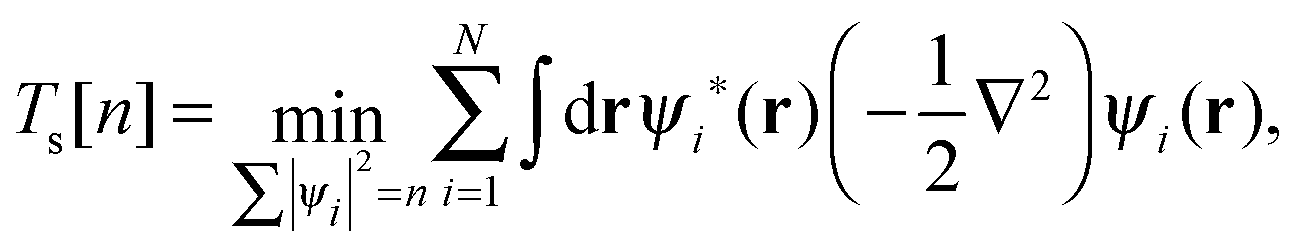
In practice, the exact form of E[n] for the many-body system is unknown and must be approximated. The Kohn–Sham (KS) approach,2 the most widely used approximation to DFT, works by introducing an equivalent non-interacting electron system for which the kinetic energy can be calculated exactly. We can define the KS kinetic functional Ts by the constrained-search formulation3 as| |  | (2) |
where the equivalent non-interacting total wave function is constructed as a Slater determinant from the single-particle orbitals ψi. Because the kinetic term is the dominant contribution to the total energy expression, introducing the exact kinetic functional ensures that the remaining terms (which need to be approximated) are comparatively small and easier to handle. This strategy allows us to derive KS density functional approximations of reasonable accuracy, especially when the balance between required computational resources and accuracy is taken into account. More precisely, in the KS method, we introduce the kinetic functional Ts, the classical electron–electron repulsive Coulombic interaction| | 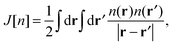 | (3) |
with the remaining contribution to the total energy denoted as “exchange correlation”. Thus, we rewrite the KS DFT energy functional as| |  | (4) |
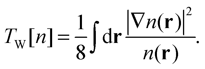
In the spirit of Hohenberg–Kohn theory, we can also introduce a kinetic functional that is explicitly density-dependent.4 This leads directly to an orbital-free (OF) formulation of the same unknown energy functional. For example, we can introduce the exact single-electron kinetic functional that is equivalent to the Weizsäcker functional TW[n]5| |  | (5) |
Another approach consists of expressing EOF[n] in terms of the KS kinetic functional Ts and the KS exchange–correlation functional Exc:4,6
| |  | (6) |
where the final term is known as the Pauli functional
Tθ. The minimum of the energy functional is found by a functional derivative subject to the constraint that the density integrates to the number of electrons
N using the Lagrange multiplier
εOF. The resulting single Euler equation is then:
4| |  | (7) |
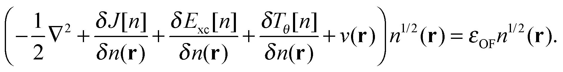
The eigenvalue εOF is equal to minus the ionization potential for the exact energy functional.4 Relying on quantities borrowed from KS theory is obviously not the only possible choice, but it allows us to build on the accumulated knowledge of the widely used KS functionals. After introducing Ts and Exc in the OF formulation of the total energy functional, the remaining task to achieve an accuracy comparable to the parent KS method is to obtain an orbital-free approximation to Ts that approaches the exact orbital-dependent KS limit.
A number of OF kinetic functionals have been proposed over the years. Typically, they are a combination of two exact ubiquitous kinetic functionals, the Thomas–Fermi7,8 and Weizsäcker5 kinetic functionals, defined as
| |  | (8) |
| |  | (9) |
The Thomas–Fermi kinetic functional is the exact kinetic functional of the homogeneous electron gas and therefore correctly reduces to
Ts in the constant density limit. To improve the description of atomic and molecular densities, Weizsäcker derived
TW as a correction to the Thomas–Fermi kinetic functional.
5 This correction was later derived from gradient expansion techniques with a different prefactor.
9 The first two terms in the gradient expansion are denoted as the TF
λW functional:
| | | TTFλW[n] = TTF[n] + λTW[n], | (10) |
with the parameter
λ = 1/9.
10,11 Weizsäcker initially proposed the value
λ = 1, whereas a later work proposed the value
λ = 1/5 by optimizing atomic and small molecule energies.
12 Other proposed values include
λ = 0.186 for the limit of large atomic number
13 and
λ = 0.12 from post-KS optimization of small molecule energies.
14
It is also reasonable to treat TW as the first term in the expansion of the KS kinetic functional Ts and include a parametrized Thomas–Fermi contribution as a correction.9,15,16 In the general form, the Thomas–Fermi functional is multiplied by a function dependent on the number of electrons N:
| | | TγTFW[n] = TW[n] + γ(N)TTF[n]. | (11) |
.
Issues with accuracy and convergence are the reasons why the development of OF kinetic functionals remains an active area of research. There are excellent recent reviews to which we refer the reader for further information on such developments.6,17–22 Here, we briefly mention a few. For example, a family of kinetic functionals has been established in analogy with the development of generalized gradient approximations (GGA) for exchange–correlation functionals. The kinetic GGA form uses in its formulation the reduced density gradient  , a Weizsäcker contribution, and a modified Thomas–Fermi functional with an enhancement factor. From the proposed GGA kinetic functionals, we can cite forms with empirical and non-empirical parameters in the enhancement factor.23–25 Moreover, the general combination of TTF and TW is also derived from quantization from classical considerations or information theoretic arguments.15,26,27 Similarly, non-local kinetic energy functionals include a sum of TTF and TW functionals that is corrected with a non-local two-point functional.18 Finally, we mention that a family of functionals is also developed and tested for embedding applications with frozen density approaches.28,29
In examining the performance of kinetic functionals, most studies have relied on the use of what could be considered good trial densities, typically from Hartree–Fock theory or KS LDA (local density approximation) calculations in non-self-consistent or post-KS treatments. While one can extract some useful information from such methods (for example, we can rule out functionals based on failures at this level), these studies have a fundamental limitation to assess the true performance of the kinetic functional, given that the self-consistent density will differ from the density actually employed. Moreover, many applications of OFDFT functionals rely on the use of pseudo-potentials that must overcome difficult problems, stemming from the essential relationship between the method and the separation of orbitals on core and valence electrons.18,22
Due to numerical difficulties, the self-consistent all-electron assessment of OF functionals typically has focused on atoms or diatomic molecules and only a small number of OF functionals have been tested.6,30–36 For example, in Chan et al.,32 the kinetic TFλW functional is used in addition to the LDA exchange for a few values of λ (λ = 1, 1/5, 1/9, 2) in self-consistent all-electron calculations using a Gaussian basis. Out of the λ values studied, the best agreement to Hartree–Fock energies is obtained for λ = 1/5, as in earlier work.12 The ionization energies increase with increasing λ, and the values computed oscillate around the experimental values. For the Ne atom, the progressive effect of increasing λ is to lower the value at the origin (position of the nucleus) and increase the density value in the valence region. From the binding energies of molecules the authors conclude that, indeed, the addition of a gradient term such as TW allows for a small binding of the molecules. This binding increases with increasing λ, but none of the tried parameters gives a satisfactory description because the errors in the atomic energy increase drastically. These binding energies of molecules are reproduced by two later studies,6,35 using different methods. The first one uses a non-modified nuclear potential and both the Gaussian and a grid basis, and the second study uses the PAW transformation and a grid basis. Notably, with the use of the PAW method bulk simulations were reported at the same level of theory.35
We have chosen to extend the benchmark data for OF all-electron self-consistent calculations for atoms. Using an all-electron radial atomic OFDFT code to compute all-electron values, we study a wide region of the parameter space of the parametrized Thomas–Fermi–Weizsäcker kinetic model. To achieve convergence for values of λ other than λ = 1, we use the potential scaling from our previous work.35 By working within this wide region in parameter space, we can achieve a deeper understanding of the interplay between the fractions of TTF and TW contained in the model that yield good agreement with the reference KS calculation. Here, total energy, eigenvalue, and all-electron densities are of interest, particularly, when the parameters λ and γ are varied between 0.2 and 1.5. We choose to compare the OFDFT results with reference KS calculations because, for the ideal case of an exact kinetic functional, all the quantities should agree. These results will bridge the way to improve the parameter transferability from atomic to dimeric systems, and in general, to the overall improvement of the OF kinetic functional derivation.
2. Results and discussion
In order to define an OF model in the KS-like form described in the Introduction, we must work under approximations for the KS kinetic and exchange–correlation functionals. Here we use a parametrized kinetic functional37 that we denote as TγTFλW in an extension of the naming convention used in the Introduction, and an LDA exchange–correlation functional.38,39 The parametrized orbital-free functional we study here is, therefore:| | | EOF[n;λ,γ] = λTW[n] + γTTF[n] + J[n] + V[n] + ELDAxc[n] | (12) |
Using the partitioning introduced in eqn (6), we obtain the KS-like equation to solve by setting:| | | Tθ[n] = (λ − 1)TW[n] + γTTF[n], | (13) |
in eqn (7). The Weizsäcker term in the Pauli functional can be expanded in its Laplacian form and combined back with the first term so that the final KS-like equation to solve is:| |  | (15) |
or in the convenient scaled form used in previous work:35| |  | (16) |
2.1 Total energy
In the ideal limit where the exact form of the KS kinetic energy functional is retrieved, both OF and KS energy functionals as defined in eqn (4) and (6) are equal. We therefore explore the evolution of the total energy of different atoms in the first three rows of the periodic table as the two parameters that define the OF kinetic energy functional introduced here are varied. By comparing the KS and OF total energies throughout this parameter space, one can determine which combinations of λ and γ yield good agreement between the two methods. A good OF kinetic functional, TγTFλW, can then be obtained by minimizing the difference between the KS and OF predicted total energies (or other properties) with respect to the choice of λ and γ. In practice, this can be done by studying the quantity| |  | (17) |
which for each atom gives the relative error in the OF total energy EOF, taking the KS value EKS as a reference, as a function of λ and γ. One can then extend this analysis to a wider set of elements by studying the cumulative error, which is simply given as the average relative error  , where a is an atom index and Na is the number of atoms included in the set. The error for each atom and the cumulative error as defined above are presented in Fig. 1. Previous work indicates that the average error in the atomic energy for parameters (λ,γ) = (1/5,1) is very small.12,32 We also find the average error in the atomic total energies calculated at (λ,γ) = (1/5,1) to be very small. In this OF model, which differs from the cited work by the inclusion of the LDA correlation, the average error for the present atomic set is only of 3 percent deviation from the KS reference values. This (λ,γ) combination is, however, not singular. It belongs to a whole region in parameter space with good agreement between the OF and KS energies, indicated in white and the superimposed dashed lines in the figure. For the H atom, such a region includes the limit (λ,γ) = (1,0) for which the Weizsäcker term is the exact kinetic energy functional. The evolution of these regions of good agreement as the atomic number increases is smooth, so that there still exists a well-defined region of overall good agreement between the OF and KS energies. We note that for every atom the (λ,γ) values corresponding to the region of good agreement can be described by means of a second-order polynomial fitting, valid within the ranges shown. These second-order expressions give optimum γs for any given λ in terms of reproducing the KS values, γopt(λ) = a2λ2 + a1λ + a0. The fitting coefficients for all the atoms studied are given in Table 1.
 |
| | Fig. 1 Evolution of the relative error in OF total energies with respect to KS reference total energies calculated for all the atoms in the first three rows of the periodic table, cf.eqn (17) for a definition. The cumulative error is calculated as the combined average error for the whole set,  . The OF kinetic functional used is λTW[n] + γTTF[n] and the exchange–correlation is a LDA functional (cf.eqn (12) for the complete energy functional). The parameters λ and γ are varied in the same range for all plots. The black region in the top-right corner for He is due to the impossibility to bring the corresponding calculations to convergence. . The OF kinetic functional used is λTW[n] + γTTF[n] and the exchange–correlation is a LDA functional (cf.eqn (12) for the complete energy functional). The parameters λ and γ are varied in the same range for all plots. The black region in the top-right corner for He is due to the impossibility to bring the corresponding calculations to convergence. | |
Table 1 Fitting parameters for the second-order polynomial γE(λ) = a2λ2 + a1λ + a0. This polynomial gives the combination of (λ,γ) yielding the OF total energies that better agree with the reference KS total energies of different atoms. The fitted curves are shown as dashed lines in Fig. 1
| Atom |
a
2
|
a
1
|
a
0
|
| H |
0.372 |
−2.386 |
2.032 |
| He |
0.272 |
−1.614 |
1.347 |
| Li |
0.305 |
−1.428 |
1.301 |
| Be |
0.207 |
−1.175 |
1.236 |
| B |
0.162 |
−1.013 |
1.195 |
| C |
0.145 |
−0.928 |
1.180 |
| N |
0.128 |
−0.859 |
1.166 |
| O |
0.145 |
−0.851 |
1.167 |
| F |
0.135 |
−0.796 |
1.147 |
| Ne |
0.129 |
−0.768 |
1.136 |
| Na |
0.165 |
−0.799 |
1.145 |
| Mg |
0.127 |
−0.718 |
1.122 |
| Al |
0.108 |
−0.672 |
1.109 |
| Si |
0.119 |
−0.676 |
1.112 |
| P |
0.113 |
−0.651 |
1.104 |
| S |
0.147 |
−0.689 |
1.117 |
| Cl |
0.128 |
−0.649 |
1.106 |
| Ar |
0.135 |
−0.648 |
1.108 |
A simple correlation between the two components of the kinetic functional can be observed. As the fraction of the Weizsäcker functional added to the model increases, so does the need to decrease the fraction of the Thomas–Fermi functional in order to achieve a good description of the total energy. As previously discussed, this correlation is not linear and it can be clearly observed how the total energy values become more insensitive to an increase of the von Weizsäcker functional contribution as the number of electrons in the system increases.
2.2 Eigenvalues
The fundamental chemical properties of atoms are determined by the process of acceptance or removal of electrons. In this context, the chemical reactivity of molecular systems and atoms, in particular, is a desired quantity to be addressed by means of the OF model. In the KS model, the highest occupied molecular orbital (HOMO) eigenvalue of the KS equations has a special physical significance.40,41 The KS HOMO eigenvalue determines the decaying behaviour of the electronic density and equals minus the ionization potential using the exact energy functional.40 The Euler equation eigenvalue in the OF model also determines the decaying behaviour of the density and equals minus the ionization potential for the exact functional.4 When having an exact approximation for the KS kinetic functional in the OF model, the two eigenvalues should coincide.4,42 Despite the poor description of the KS frontier eigenvalues, observed for both local and semi-local exchange–correlation approaches, reproducing the KS results is a first step in the construction of better kinetic functionals for the OF model. In this section, we study the behaviour of the OF eigenvalue for the same atomic species surveyed in the previous section, and compare it to the KS HOMO eigenvalue. The error is defined in a similar way to the total energy case as a relative deviation from the KS reference for different values of λ and γ, writing the eigenvalue as ε(λ,γ), it reads| |  | (18) |
where the cumulative error is defined in a similar way to the error in the total energy as the average relative error  . Here, a is an atom index and Na is the number of atoms in the set. Fig. 2 shows the error in the eigenvalue for each atomic species. The results show that the best set of parameters behave differently compared to the error in the total energy. For low values of the parameter γ, there already exists an underestimation of the OF eigenvalue (the error is negative) and no value of λ can decrease the error. However, at moderate and high values of γ and at low λ, the eigenvalue error is positive so that the OF eigenvalues are an overestimation of the KS eigenvalue. Increasing λ decreases the OF eigenvalue up to the point where it matches the KS eigenvalue. If λ is further increased, the OF eigenvalue just continues to deviate from the KS value.
 |
| | Fig. 2 Evolution of the relative error in OF eigenvalue with respect to the KS HOMO calculated for all the atoms in the first three rows of the periodic table, cf.eqn (18) for a definition. The cumulative error is calculated as the combined average error for the whole set,  . The OF kinetic functional used is λTW[n] + γTTF[n] and the exchange–correlation is a LDA functional (cf.eqn (12) for the complete energy functional). The parameters λ and γ are varied in the same range for all plots. . The OF kinetic functional used is λTW[n] + γTTF[n] and the exchange–correlation is a LDA functional (cf.eqn (12) for the complete energy functional). The parameters λ and γ are varied in the same range for all plots. | |
Another striking difference between the total energy and the eigenvalue is that the calculated region of best agreement strongly depends on the atom. In particular, the best regions for H and He show a distinctly different behaviour when compared to the other atoms. This is because both species are single-orbital systems and they are well described by the Weizsäcker model, which corresponds to the values of (λ,γ) = (1,0). In general, a best set of parameters can be chosen to describe elements with similar chemical properties (with the same number of valence electrons, i.e. elements in the same column of the periodic table). The superposition therefore does lead to a high average error (more than 40 percent) in comparison to the total energy. It is interesting to note that the error at the pair of parameters (λ,γ) = (1/5,1) is quite high (48 percent). Furthermore, this parameter pair does not belong to the fitted region of best agreement that can be observed in the cumulative graph. For each atomic species, the parameter region of the lowest error has been fitted, as the energy, to a second-order polynomial (red-dashed line), and the coefficients are included in Table 2.
Table 2 Fitting parameters for the second-order polynomial γε(λ) = a2λ2 + a1λ + a0. This polynomial gives the combination of (λ,γ) yielding the OF eigenvalue that better agree with the reference KS HOMO of different atoms. The fitted curves as shown as dashed lines in Fig. 2
| Atoms |
a
2
|
a
1
|
a
0
|
| H |
−0.607 |
0.161 |
0.407 |
| He |
−0.422 |
0.202 |
0.203 |
| Li |
−0.351 |
0.992 |
0.811 |
| Be |
−0.188 |
0.625 |
0.469 |
| B |
−0.215 |
0.852 |
0.657 |
| C |
−0.179 |
0.710 |
0.479 |
| N |
−0.152 |
0.616 |
0.383 |
| O |
−0.152 |
0.573 |
0.319 |
| F |
−0.136 |
0.519 |
0.278 |
| Ne |
−0.109 |
0.455 |
0.255 |
| Na |
−0.794 |
1.579 |
0.751 |
| Mg |
−0.162 |
0.803 |
0.542 |
| Al |
−0.955 |
1.726 |
0.742 |
| Si |
−0.230 |
0.958 |
0.578 |
| P |
−0.151 |
0.759 |
0.474 |
| S |
−0.137 |
0.682 |
0.392 |
| Cl |
−0.131 |
0.636 |
0.331 |
| Ar |
−0.109 |
0.563 |
0.302 |
We can then conclude that achieving small errors for both energy and eigenvalue is not possible with this simple parameterization. In order to achieve the best possible chemical accuracy for a specific problem of interest, one can however optimize this parametrization such that the resulting functional minimizes both errors for each atom or for a small set of atoms.
2.3 Electronic density
The OF and KS electronic densities should coincide if an exact approximation of the KS kinetic functional is used in the OF functional. To characterize the error we have used the following definition:| | 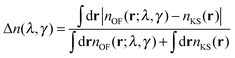 | (19) |
where the denominator reduces to 2Z for the neutral atomic densities considered here (where Z is the atomic number). The cumulative error is defined as earlier by  , where a is an atom index and Na is the number of atoms in the set. From the definition we expect that the regions of high density will dominate this integrated error and therefore the error will reflect the core density error rather than the error in the decaying tail.
As is the case for the total energy error, Fig. 3 shows there is a different dependence for each atom of the region of best agreement. However, it tends to quickly converge when increasing the number of electrons. The average error is therefore quite homogeneous (at 0.15 to 0.20 |e| per electron). Contrary to the total energy and eigenvalue cases, a wide range of parameters allow us to approach the KS density with a similar error. The maximum possible deviation is 1 so that it can also be interpreted as a percentage (multiplying the error by 100). An average error of 15 to 20 percent is a poor feature that was similarly encountered in the eigenvalue error. We can therefore conclude that for the present parametrization and for atoms, the integrated density error is a quantity that can be omitted from a fitting procedure without much loss with respect to improving the functional. Other density-dependent error quantities may be more sensitive to the parameters and further exploration is required.
 |
| | Fig. 3 Deviation of the OF density with respect to the KS density for atoms. The maximum deviation is 1 and it would correspond to a situation of complete no overlap of the densities. On the right-hand side, the combined cumulative error (or mean error) for the set of atoms is included. The OF kinetic functional used is λTW[n] + γTTF[n] and the exchange–correlation is a LDA functional (cf.eqn (12) for the complete energy functional). The parameters λ and γ are varied in the same range for all plots. | |
2.4 N2 molecule
We focused on the nitrogen dimer as an example of the diatomic molecule where we can study the error in the molecule formation using parameters obtained from our previous atomic results. The nitrogen dimer is also studied in detail in one of the OF all-electron studies we use as reference.32 In that all-electron reference, they proved that adding the Weizsäcker functional in the kinetic functional helped to overcome the no-binding failure of the Thomas–Fermi kinetic model. However, with the parameters (λ,γ) = (1/5,1) fitted to atomic energies the binding energy obtained was very small and the bond distance was completely overestimated with respect to a HF calculation. By increasing λ, and using (λ,γ) = (2,1), they obtained a good value for the bond length but at the price of having the binding energy overestimated. Here, we use parameters coming from our own fits γE (coefficients from the energy fit in Table 1 for the N atom) and γε (coefficients from the eigenvalue fit from Table 2 for the N atom) to study the binding energy, bond length distance and eigenvalue of the N2 molecule. We use rcut = 1.0 Bohr and grid spacing h = 0.14 Å in the setup generation and GPAW calculation respectively.
Table 3 summarizes the N2 results. We tested first two pairs of parameters with same λ but different γ, one γ fitted to reproduce the KS atomic energy and the other γ fitted to reproduce the KS HOMO eigenvalue. The result is that the kinetic functional with parameters fitted to reproduce the atomic KS eigenvalue reproduces the dimer KS bond distance better (the error is 0.1 Å, while the other one gives an error of 0.6 Å). We tested another value of γ, this time close to the value reported in the reference. Setting λ = 2, the γε fitted to reproduce the KS HOMO eigenvalue equals 1.007, a value very close to the one reported by Chan et al.32 With those parameters, we obtained good bond distances but again bad binding energies. The error is 0.08 Å and 26 eV for bond and binding respectively. Finally, we used the parameters in the intersection of the two optimum curves and obtained simultaneously a lower error in both quantities, 0.2 Å and 2.7 eV for bond and binding respectively. For practical applications, however, the errors obtained with the parameters optimized for energy and eigenvalue simultaneously are unacceptable. With applications in mind, we should still decrease the error by fine-tuning the parameters or even trying other equivalent training sets (for example, electronegativity, electron affinity or direct evaluation of the ionization potential). Our main conclusion here is that in order to improve the kinetic functional transferability from atoms to molecules, the kinetic functional must correctly describe the tendency to donate electrons at the atomic level. This conclusion now requires a systematic exploration using more molecules, molecular properties and using a wider range of parameter space.
Table 3 Binding energies in eV (BE = 2E(N) − E(N2)), optimized bond length in Å and eigenvalue in eV of the N2 molecule for various parameters in the kinetic OF functional λTW + γTTF. The LDA exchange–correlation functional is composed of the Dirac exchange and PW correlation.38,39 The KS reference values are calculated with the same exchange–correlation in a spin-polarized formalism using GPAW
| Method and parameters |
BE |
r
e
|
Eigenvalue |
| OF (λ,γE) = (1.000,0.435) |
87.488 |
0.534 |
−21.829 |
| OF (λ,γε) = (1.000,0.847) |
21.062 |
0.991 |
−8.172 |
| OF (λ,γε) = (2.000,1.007) |
37.398 |
1.010 |
−9.294 |
| OF (λ,γE ∩ γε) = (0.599,0.697) |
14.383 |
0.903 |
−8.057 |
|
|
| KS LDA |
11.663 |
1.093 |
−10.418 |
2.5 Convergence tests
In our calculations, we have used the all-electron radial atomic code that is included in the DFT code GPAW43 and that was previously modified to self-consistently solve the OF minimization problem.35 The atomic all-electron code in GPAW is used as a generator of the atomic all-electron orbitals necessary for the generation of the PAW transformation. In our previous work,35 we presented the parameters for the calculations of a small set of atoms. Here we extend systematically our convergence tests to the atoms in the first two rows of the periodic table. We have used in the calculations presented in the previous sections the GPAW parameters gpernode and mix set to 800 and 0.01, respectively, in the all-electron atomic code. These parameters determine the number of points in the atomic radial grid and the degree of mixing between old and new potentials during the self-consistency cycle. In order to test the energy deviation with respect to the reference all-electron values32 for the selected atoms, the λ and γ values were set to 0.2 and 1.0, respectively. Taking the energy value E from the literature32 as a reference, the deviation ΔE of the calculated total energy EOF for an atom can be expressed as Note that in this section we use Bohr units for rcut (the radius of the PAW augmentation sphere), because these are the units used in the PAW setup generation. The grid calculation energy values are given in eV.
As seen from Fig. 4 the energy deviation for selected atoms does not exceed the absolute value of 0.007 eV. Thus, the gpernode = 800 value was used for extending the convergence tests to the PAW setup generator.
 |
| | Fig. 4 Energy deviation with respect to the reference value32 calculated for the first and second row elements for gpernode = 800, λ = 0.2, 1.0, and rcut = 1.2 Bohr. | |
We can use the benchmark data we have obtained in addition to data from the literature to study the PAW generation parameter rcut and the parameters for the evaluation of this model on the grid using the PAW transformation (grid spacing h). The rcut parameter determines the size of the augmentation sphere and therefore the size of the region where the PAW transformation will be defined. For each atom, we study the set of parameters (λ,γ) = (1,1).
The total energy deviation obtained from eqn (20) for the H and O atoms as a function of rcut is presented in Fig. 5. It is found that for the first and second row elements of the periodic table the energy deviation converges to the reference value with an rcut value equal to 1.2 Bohr, for all the tested grid spacings. For instance, for the H atom, at rcut = 1.2 Bohr, the maximum energy deviation was found to be about 0.007 eV for h = 0.2 Å, compared to 0.005 eV for h = 0.12 Å, while the computation time was about one order of magnitude shorter. Above rcut = 1.2 Bohr, the grid atomic energy shows very little dependence on the grid spacing. In conclusion, a grid spacing of 0.18 Å could be used to save the computational time with such an rcut. Below rcut = 1.2 Bohr, the grid spacing needs to be decreased until convergence of the atomic energy is achieved. In this region the energy deviation increases as one reaches heavier atoms. As seen in Fig. 5(b), for example, for the O atom, using an rcut equal to 1.0 Bohr, the energy deviation is found to converge at h = 0.14 Å (energy difference of −0.017 eV). To test the parameters for the PAW generation for systems other than atoms and below rcut = 1.2 Bohr, one needs to test the convergence of energy differences (such as binding energy).43 This is exactly the case of the N2 molecule studied in the last section. The LDA bond length (and the expected bond length) is of only 1.093 Å. An rcut = 1.0 Bohr (=0.53 Å) therefore, would not induce augmentation sphere superposition errors at such a distance. We then test the deviation with respect to the all-electron binding energy reference,32 when varying the grid parameter h. We obtained the error −0.075, −0.081 and −0.082 eV with a grid spacing of 0.18, 0.14 and 0.12 Å respectively. We then determined that binding energy is converged for a grid spacing of 0.14 Å and that the error with respect to all-electron reference is small. We have therefore chosen the grid spacing of 0.14 Å for our dimer calculations. A systematic study of binding energy convergence for a wider set of molecules will be presented in our next study.
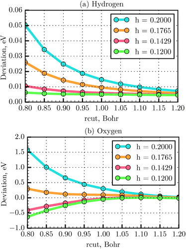 |
| | Fig. 5 Convergency of total energy with respect to all-electron energy using TFD1W theory for various rcut values and different grid spacings, calculated for the H (a) and O (b) atoms, respectively. | |
3. Conclusions
Using an all-electron radial atomic orbital-free DFT code,35 we have studied the performance of a parametrized OF model. In the model we include a parametrized Thomas–Fermi–Weizsäcker kinetic functional, where λ and γ determine the amount of Weizsäcker and Thomas–Fermi functionals added to the model, respectively, in addition to an LDA exchange–correlation. We have studied the interplay between λ and γ in terms of achieving an agreement between the OF calculation and the corresponding KS calculation. We have compared the OFDFT results to the equivalent KSDFT results following the rationale that for a perfect KS kinetic functional approximation, quantities such as total energy, Euler equation eigenvalue and electronic density should agree completely.
As the fraction of the Weizsäcker functional added to the model increases, so does the need to decrease the fraction of the Thomas–Fermi functional in order to achieve a good description of the total energy. In contrast, the best region of agreement for the eigenvalue strongly depends on the particular atom. The atomic density error shows a similar dependence but converges fast towards a homogenous error when the atomic number increases.
For the total energy and eigenvalue, we have fitted the regions of best agreement with a γ function that is not linear but quadratic. The fitted parameters for the total energy and eigenvalue interpolation formulas are essentially different. We can use the fitted coefficients to derive a small set of parameters per atom or for a small set of atoms that minimize both total energy and eigenvalue errors. However, any pair of parameters in this parametrized functional form will present large errors on average for the eigenvalue and the density of the different elements/molecules belonging to any sizeable system set. As an application of the atomic analysis, we tested a dimer formation with kinetic functionals fitted to reproduce the atomic total energy and the eigenvalue. We determined that a kinetic functional fitted to energy and eigenvalue simultaneously gave a smaller error in the binding energy, bond length and eigenvalue that kinetic functionals fitted to reproduce only one of the atomic properties.
These results regarding the performance of a parametrized OF functional within a wide region in parameter space can now open the way to test the parameter transferability and the overall accuracy of parametrized OF density functionals.
Acknowledgements
This work was supported by the Academy of Finland projects 279240 and 251748. We are grateful to CSC, the Finnish IT Center for Science in Espoo, and the Applied Physics Department of Aalto University for computational resources.
References
- P. Hohenberg and W. Kohn, Phys. Rev., 1964, 136, B864–B871 CrossRef.
- W. Kohn and L. J. Sham, Phys. Rev., 1965, 140, A1133–A1138 CrossRef.
-
Density Functionals for Coulomb Systems, in Physics as Natural Philosophy, ed. A. Shimony and H. Feshbach, M.I.T. Press, 1982, pp. 111–149 Search PubMed.
- M. Levy, J. P. Perdew and V. Sahni, Phys. Rev. A: At., Mol., Opt. Phys., 1984, 30, 2745–2748 CrossRef.
- C. Weizsäcker, Z. Phys., 1935, 96, 431–458 CrossRef.
- V. Karasiev and S. Trickey, Comput. Phys. Commun., 2012, 183, 2519–2527 CrossRef CAS PubMed.
- L. H. Thomas, Math. Proc. Cambridge Philos. Soc., 1927, 23, 542–548 CrossRef CAS.
- E. Fermi, Rend. Accad. Lincei, 1927, 6, 602–607 CAS.
-
R. Parr and W. Yang, Density-Functional Theory of Atoms and Molecules, Oxford University Press, USA, 1989 Search PubMed.
- D. A. Kirzhnitzs, Sov. Phys. JETP, 1957, 5, 64–71 Search PubMed.
- C. H. Hodges, Can. J. Phys., 1973, 51, 1428–1437 CrossRef.
- K. Yonei and Y. Tomishima, J. Phys. Soc. Jpn., 1965, 20, 1051–1057 CrossRef CAS.
- E. H. Lieb, Rev. Mod. Phys., 1981, 53, 603–641 CrossRef CAS.
- A. Borgoo, J. A. Green and D. J. Tozer, J. Chem. Theory Comput., 2014, 10, 5338–5345 CrossRef CAS.
- S. Sears, R. Parr and U. Dinur, Isr. J. Chem., 1980, 19, 165–173 CrossRef CAS PubMed.
- J. Gázquez and E. Ludeña, Chem. Phys. Lett., 1981, 83, 145–148 CrossRef.
-
V. Karasiev, D. Chakraborty and S. Trickey, in Many-Electron Approaches in Physics, Chemistry and Mathematics, ed. V. Bach and L. Delle Site, Springer International Publishing, 2014, pp. 113–134 Search PubMed.
- J. Xia, C. Huang, I. Shin and E. a. Carter, J. Chem. Phys., 2012, 136, 084102 CrossRef PubMed.
-
V. V. Karasiev, R. S. Jones, S. B. Trickey and F. E. Harris, in New Developments in Quantum Chemistry, ed. J. Luis Paz and A. J. Hernndez, Transworld Research Network, Kerala, India, 2009, pp. 25–54 Search PubMed.
- G. Ho, C. Huang and E. Carter, Curr. Opin. Solid State Mater. Sci., 2007, 11, 57–61 CrossRef CAS PubMed.
- H. Chen and A. Zhou, Numer. Math. Theor. Meth. Appl., 2008, 1, 1–28 Search PubMed.
- D. R. Bowler and T. Miyazaki, Rep. Prog. Phys., 2012, 75, 036503 CrossRef CAS PubMed.
- F. Tran and T. A. Wesolowski, Int. J. Quantum Chem., 2002, 89, 441–446 CrossRef CAS PubMed.
- A. Lembarki and H. Chermette, Phys. Rev. A: At., Mol., Opt. Phys., 1994, 50, 5328–5331 CrossRef CAS.
- V. V. Karasiev, D. Chakraborty, O. A. Shukruto and S. B. Trickey, Phys. Rev. B: Condens. Matter Mater. Phys., 2013, 88, 161108 CrossRef.
- I. P. Hamilton, R. A. Mosna and L. D. Site, Theor. Chem. Acc., 2007, 118, 407–415 CrossRef CAS PubMed.
- L. M. Ghiringhelli and L. Delle Site, Phys. Rev. B: Condens. Matter Mater. Phys., 2008, 77, 073104 CrossRef.
- C. R. Jacob, J. Neugebauer and L. Visscher, J. Comput. Chem., 2008, 29, 1011–1018 CrossRef CAS PubMed.
- T. A. Wesolowski, H. Chermette and J. Weber, J. Chem. Phys., 1996, 105, 9182 CrossRef CAS PubMed.
- Y. Tomishima and K. Yonei, J. Phys. Soc. Jpn., 1966, 21, 142–153 CrossRef CAS.
- W. Yang, Phys. Rev. A: At., Mol., Opt. Phys., 1986, 34, 4575–4585 CrossRef.
- G. K.-L. Chan, A. J. Cohen and N. C. Handy, J. Chem. Phys., 2001, 114, 631–638 CrossRef CAS PubMed.
- B. M. Deb and P. K. Chattaraj, Phys. Rev. A: At., Mol., Opt. Phys., 1988, 37, 4030–4033 CrossRef CAS.
- P. K. Chattaraj, Phys. Rev. A: At., Mol., Opt. Phys., 1990, 41, 6505–6508 CrossRef CAS.
- J. Lehtomäki, I. Makkonen, M. A. Caro, A. Harju and O. Lopez-Acevedo, J. Chem. Phys., 2014, 141, 234102 CrossRef PubMed.
- M. D. Glossman, A. Rubio, L. C. Balbs and J. A. Alonso, Phys. Rev. A: At., Mol., Opt. Phys., 1993, 47, 1804–1810 CrossRef CAS.
- W.-J. Yin and X.-G. Gong, Phys. Lett. A, 2009, 373, 480–483 CrossRef CAS PubMed.
- P. A. M. Dirac, Proc. Cambridge Philos. Soc, 1930, 26, 376 CrossRef CAS.
- J. P. Perdew and Y. Wang, Phys. Rev. B: Condens. Matter Mater. Phys., 1992, 45, 13244–13249 CrossRef.
- J. P. Perdew and A. Zunger, Phys. Rev. B: Condens. Matter Mater. Phys., 1981, 23, 5048–5079 CrossRef CAS.
- J. Janak, Phys. Rev. B: Condens. Matter Mater. Phys., 1978, 18, 7165–7168 CrossRef CAS.
- M. Levy and H. Ou-Yang, Phys. Rev. A: At., Mol., Opt. Phys., 1988, 38, 625–629 CrossRef.
- J. J. Mortensen, L. B. Hansen and K. W. Jacobsen, Phys. Rev. B: Condens. Matter Mater. Phys., 2005, 71, 035109 CrossRef.
Footnote |
| † Electronic supplementary information (ESI) available. See DOI: 10.1039/c5cp01211b |
|
| This journal is © the Owner Societies 2015 |
Click here to see how this site uses Cookies. View our privacy policy here. 
 Open Access Article
 This Open Access Article is licensed under a
  *a
*a


 , a Weizsäcker contribution, and a modified Thomas–Fermi functional with an enhancement factor. From the proposed GGA kinetic functionals, we can cite forms with empirical and non-empirical parameters in the enhancement factor.23–25 Moreover, the general combination of TTF and TW is also derived from quantization from classical considerations or information theoretic arguments.15,26,27 Similarly, non-local kinetic energy functionals include a sum of TTF and TW functionals that is corrected with a non-local two-point functional.18 Finally, we mention that a family of functionals is also developed and tested for embedding applications with frozen density approaches.28,29


 , where a is an atom index and Na is the number of atoms included in the set. The error for each atom and the cumulative error as defined above are presented in Fig. 1. Previous work indicates that the average error in the atomic energy for parameters (λ,γ) = (1/5,1) is very small.12,32 We also find the average error in the atomic total energies calculated at (λ,γ) = (1/5,1) to be very small. In this OF model, which differs from the cited work by the inclusion of the LDA correlation, the average error for the present atomic set is only of 3 percent deviation from the KS reference values. This (λ,γ) combination is, however, not singular. It belongs to a whole region in parameter space with good agreement between the OF and KS energies, indicated in white and the superimposed dashed lines in the figure. For the H atom, such a region includes the limit (λ,γ) = (1,0) for which the Weizsäcker term is the exact kinetic energy functional. The evolution of these regions of good agreement as the atomic number increases is smooth, so that there still exists a well-defined region of overall good agreement between the OF and KS energies. We note that for every atom the (λ,γ) values corresponding to the region of good agreement can be described by means of a second-order polynomial fitting, valid within the ranges shown. These second-order expressions give optimum γs for any given λ in terms of reproducing the KS values, γopt(λ) = a2λ2 + a1λ + a0. The fitting coefficients for all the atoms studied are given in Table 1.

 . The OF kinetic functional used is λTW[n] + γTTF[n] and the exchange–correlation is a LDA functional (cf.eqn (12) for the complete energy functional). The parameters λ and γ are varied in the same range for all plots. The black region in the top-right corner for He is due to the impossibility to bring the corresponding calculations to convergence.
 . Here, a is an atom index and Na is the number of atoms in the set. Fig. 2 shows the error in the eigenvalue for each atomic species. The results show that the best set of parameters behave differently compared to the error in the total energy. For low values of the parameter γ, there already exists an underestimation of the OF eigenvalue (the error is negative) and no value of λ can decrease the error. However, at moderate and high values of γ and at low λ, the eigenvalue error is positive so that the OF eigenvalues are an overestimation of the KS eigenvalue. Increasing λ decreases the OF eigenvalue up to the point where it matches the KS eigenvalue. If λ is further increased, the OF eigenvalue just continues to deviate from the KS value.

 . The OF kinetic functional used is λTW[n] + γTTF[n] and the exchange–correlation is a LDA functional (cf.eqn (12) for the complete energy functional). The parameters λ and γ are varied in the same range for all plots.
 , where a is an atom index and Na is the number of atoms in the set. From the definition we expect that the regions of high density will dominate this integrated error and therefore the error will reflect the core density error rather than the error in the decaying tail.


