Quantum chemical calculations of ³¹P NMR chemical shifts: scopes and limitations

Abstract

The aim of this work is to convince practitioners of ³¹P NMR methods to regard simple GIAO quantum chemical calculations as a safe tool in structural analysis of organophosphorus compounds. A comparative analysis of calculated GIAO versus experimental ³¹P NMR chemical shifts (CSs) for a wide range of phosphorus containing model compounds was carried out. A variety of combinations (at the HF, DFT (B3LYP and PBE1PBE), and MP2 levels using 6-31G(d), 6-31+G(d), 6-31G(2d), 6-31G(d,p), 6-31+G(d,p), 6-311G(d), 6-311G(2d,2p), 6-311++G(d,p), 6-311++G(2d,2p), and 6-311++G(3df,3pd) basis sets) were tested. On the whole, it is shown that, in contrast to what is claimed in the literature, high level of theory is not needed to obtain rather accurate predictions of ³¹P CSs by the GIAO method. The PBE1PBE/6-31G(d)//PBE1PBE/6-31G(d) level can be recommended for express estimation of ³¹P CSs. The PBE1PBE/6-31G(2d)//PBE1PBE/6-31G(d) combination can be recommended for routine applications. The PBE1PBE/6-311G(2d,2p)//PBE1PBE/6-31+G(d) level can be proposed to obtain better results at a reasonable cost. Scaling by linear regression parameters significantly improves results. The results obtained using these combinations were demonstrated in ³¹P CS calculations for a variety of medium (large) size organic compounds of practical interest. Care has to be taken for compounds that may be involved in exchange between different structural forms (self-associates, associates with solvent, tautomers, and conformers). For phosphorus located near the atoms of third period elements ((CH₃)₃PS and P(SCH₃)₃) the impact of relativistic effects may be notable.

---

Introduction

Nowadays the GIAO method allows calculation of ¹H/¹³C/¹⁵N chemical shifts (CSs) with high accuracy at a relatively modest level of theory and it can be used for a variety of structural applications.^1–15 Moreover, its quality is also good enough to determine finer structural differences such as isomeric, conformational or tautomeric structures.^16–35

Having strong evidence that the ¹H/¹³C/¹⁵N GIAO calculations are reliable and very helpful in practice, it would be also desirable to extend the approach to other nuclei. From this point of view ³¹P CSs are very attractive because, on the one hand, phosphorus is contained in many practically important compounds of organic, bioorganic and inorganic chemistry. On the other hand, the ³¹P CS is extremely sensitive to the electronic structure and range within 1000 ppm, therefore even small changes in the structure are strongly reflected in its CS.³⁶ Thus, if there was a reliable method to predict ³¹P CSs, it could be useful as an additional tool for structural elucidation of novel phosphorus containing compounds.

However, despite the great need for such a tool, it is still unclear if ³¹P CSs calculated in the framework of the GIAO method are reliable. In fact, there are relatively few reports on ³¹P NMR CS calculations using quantum chemical methods.^37–55 In several systematic studies it was shown^48–55 that a satisfactory agreement between calculations and experiments is observed when quite a “heavy” basis set or high level of theory‡ was used although deviations and exceptions were also found. It is necessary to stress that all these studies were focused only on the restricted types of small size compounds.

Summarizing the literature one can conclude that obviously there is some progress in quantum chemical ³¹P CS calculations. However some methodological questions are still left to be answered concerning the scopes and limitations of the method, in particular for practical applications. Moreover, if to take into account that authors used either high levels of theory or very “heavy” basis sets it can hardly be applied to medium and large size compounds of practical interest.

Nevertheless in spite of limitations, it seems that with some care the method can be applied at least to phosphorus in most types of environment, although several problems have to be cleared up. First, the additional shell in phosphorus may complicate the calculation of NMR parameters in frames of the GIAO method or may necessitate using “reach” basis sets and/or high level of theory, which may dramatically increase computational requirements, and as a result, it may become inapplicable to real size organic compounds. Therefore there should be some compromise between the cost and the quality, and it seems that for a variety of systems “cheaper” calculations may be sufficient.

Second, in most cases the shielding calculations are performed for individual molecules, i.e. actually vacuum conditions are modeled, when there are no collisions and interactions with other molecules. This raises the question of how the data obtained in the vacuum will apply to solutions.

Third, in practice one operates not by shielding but with CSs, which for phosphorus are referenced in respect of 75% H₃PO₄ in water. However, no data are available for this standard in the gas phase, which at first glance makes it difficult to use this compound as a reference in the calculations.

In this work we try to analyze the influence of the level of theory (CS//geometry) on the quality of CSs with the aim of finding the compromise of being “light” enough to be applied to large compounds and still giving precision of practical value. To achieve this goal we will be guided by the next “road map” that comprises three goal-driven questions: (1) is it possible to calculate ³¹P CSs with reasonable accuracy, and what is the minimum level of theory required? (2) Will the required level of theory (applied to small models) be applicable to “not small” organophosphorus compounds of practical interest? (3) What are complicated cases?

Results and discussion

There are several factors that influence the results of calculations and thus the agreement between experimental and calculated values. In reality, it can be hardly expected that theoretical data will agree well in absolute values with the experimental ones because of systematic errors and reference problems inherent to calculations. Therefore at the first stage, the goodness of used “combination” (CS//geometry) will be quantified by the squared correlation coefficient (R²) between calculated and experimental sets. Thus the higher R² will mean that the correlation of the calculated versus experimental CSs is closer to linearity although they may deviate in absolute values (i.e. the linear approximation line will not cross the co-ordinate origin or its slope will not be equal to 1). The last problem may be well resolved then by referencing to the secondary reference or by an empirical correction to account for the systematic error (vide infra).

The problem of the optimal choice for “combination” is the key point in CS calculations. These calculations consist of two steps: geometry optimization followed by the magnetic shielding calculation. Therefore, the first task is to find the optimal method for geometry optimization, which is then used in the CS calculations. Second, the influence of level of theory on the resulting CSs should be analyzed. To this end, the calculations using the small model molecules (Fig. 1) that cover a wide range of structural types and particularities in organophosphorus chemistry were run with different “combinations”. Theoretically calculated data have to be compared with gas-phase absolute shielding values. However, on the one hand, there are only very few models for which gas-phase data are available. On the other hand, almost all ³¹P NMR measurements are carried out in solution. Therefore, the solution CSs referenced to H₃PO₄ were used in correlation analysis. The calculated absolute shielding values were converted into CSs by referencing to H₃PO₄ calculated under the same conditions. This combination of the gas-phase and the solution data poses some problems that will be discussed especially in the paper below. The test set of molecules excludes H₃PO₄ itself.

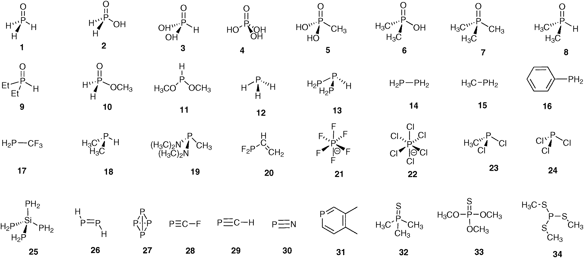Fig. 1 Structures of model compounds.

Influence of the combination on calculated chemical shifts

Variation of the method to optimize geometry. First, the level of theory was kept constant for CS calculations and was varied for geometry optimization. HF, DFT and MP2 levels of theory using a variety of basis sets starting from simple 6-31-G(d) up to 6-311++G(3df,3pd) were used for optimization. In addition, the difference between the two most popular functionals (PBE1PBE and B3LYP) was also checked. To ensure, two sets of data were obtained by using two levels to calculate CSs (PBE1PBE/6-31G(d) and PBE1PBE/6-311++G(2d,2p)).

On the whole, calculated data for most of the model compounds at different levels of theory (for geometry optimization) correlate well with experimental values, e.g. in Fig. 2a the plot of calculated (PBE1PBE/6-31G(d)//PBE1PBE/6-31G(d)) versus experimental ³¹P CSs is shown (results of the calculations for selected combinations are given in Table 1). The correlation coefficient (R²) is high enough (0.93) although in several cases there is a notable deviation from the line. It is worth stressing that there are two points that lie in very low/high field regions (−525.0 (P₄, 27) and 494.0 (P₂H₂, 26) ppm) that inevitably increase the R² value due to the large band of correlated data (Table S1, ESI†) and thus masks discrepancies in the main region. To analyze in more detail this significant part of the plot, R² values with the exception of extremely low/high field regions were recalculated (second column Table S1, ESI†). Indeed R² values become lower (0.874–0.927) in these cases. As one can see (Fig. 2a) there are several points that deviate remarkably from linear correlation: −298.2 ([PCl₆]⁻, 22), −143.7 ([PF₆]⁻, 21), −207.0 (FCP, 28), −13.9 (H₃PO, 1), 191.2 (CH₃PCl₂, 23), 275 (PN, 30), 217 (PCl₃, 24), 124.5 (P(SCH₃)₃, 34) and 59.1 ((CH₃)₃PS, 32) ppm. The variation of parameters at geometry optimization and magnetic shielding calculations do not improve correlations (Tables S1 and S2, ESI†) and these points always deviate remarkably from the rest of the cases. Probably in these points either additional effects interfere or the GIAO method fails to work well. Therefore these “difficult points” were excluded from the correlation analysis so far, and we consider the possible reasons for that disagreement in more detail later. Thus, except these latter compounds, the correlation improves notably for the rest of the 23 models (Fig. 2b). These “normal” models were used for further analysis in order to reveal key factors that influence the quality of calculated ³¹P CSs.

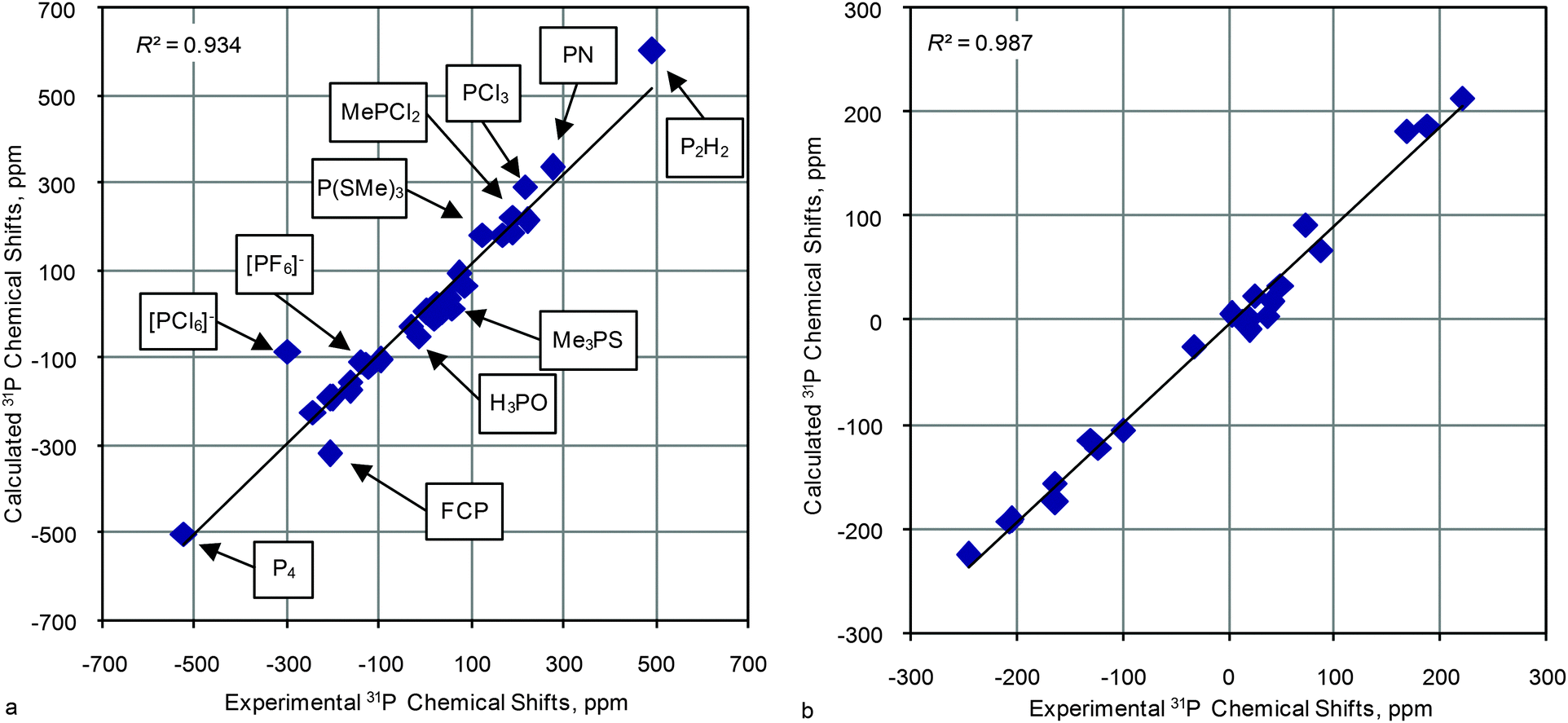Fig. 2 Correlation of calculated (PBE1PBE/6-31G(d)//PBE1PBE/6-31G(d)) versus experimental ³¹P CSs for the title compounds: (a) for all model compounds and (b) except “difficult cases” and data for very low/high field regions.

Table 1 Calculated^a (at selected levels of theory)^b and experimental ³¹P NMR CSs^c for 1–34

No.	Compound	6-31G(d)//6-31G(d)^b		6-31G(2d)//6-31G(d)^b		6-311G(2d,2p)//HF/6-31G(d)^a^,^b		6-311G(2d,2p)//6-31+G(d)^b		Exp.	Solvent	Ref.
		Unscaled	Scaled	Unscaled	Scaled	Unscaled	Scaled	Unscaled	Scaled
a DFT PBE1PBE was used, except for the third column, where HF/6-31G(d) was used for geometry optimization. b First row – the basis set used for CS calculation, second row – the basis set used for geometry optimization. c In ppm, referenced to H3PO4. d R ^2 and RMSE are the correlation coefficient and the root-mean-square error, respectively; calculated without a low/high field region and difficult cases (in italic). e Linear regression parameters (data for all combination are given in the ESI). f Not available.
1	H 3 PO	−49.4	−50.5	−84.5	−56.4	−62.7	−51.2	−71.2	−53.0	−13.9	H 2 O	56
2	H3PO2	−0.2	3.1	−25.8	4.1	−1.4	5.9	−9.1	4.9	12.5	H2O	57
3	H3PO3	6.0	9.8	−8.5	21.9	3.5	10.6	2.5	15.7	3.0	HCl	58
4	H 3 PO 4	0.0	3.3	0.0	30.7	0.0	7.3	0.0	13.4	0.0	H 2 O	59
5	CH3P(O)(OH)2	24.1	29.5	17.2	48.4	28.9	34.2	29.0	40.4	24.8	H2O	60
6	(CH3)2P(O)OH	34.0	40.3	21.7	53.0	42.1	46.5	39.4	50.1	49.4	CH3OH	61
7	(CH3)3PO	4.9	8.6	−13.3	17.0	14.9	21.2	6.7	19.6	36.2	C6H6	62
8	(CH3)2P(O)H	−8.4	−5.9	−31.0	−1.3	−4.5	3.0	−11.7	2.5	20.5	CH3OH	63
9	(CH3CH2)2P(O)H	17.8	22.7	−5.4	25.1	18.6	24.7	13.2	25.7	41.0	CHCl3	64
10	H2P(O)OCH3	2.9	6.4	−22.5	7.5	−4.6	3.0	−7.5	6.4	19.2	C6H6	65
11	HP(OCH3)2	166.8	185.0	146.7	181.8	194.8	189.0	172.8	174.4	171.5	na^f	66
12	PH3	−225.1	−241.9	−264.7	−241.9	−269.0	−243.7	−284.7	−251.9	−266.1	Gas phase	67
13	(H2P)2PH	−137.5	−146.5	−179.8	−154.5	−205.2	−184.2	−178.1	−152.6	−162.6	(CH3)2CO	68
14	(H2P)2	−191.2	−205.0	−233.6	−209.9	−229.1	−206.5	−239.1	−209.5	−203.6	(CH3)2CO	68
15	H2PCH3	−155.9	−166.6	−191.7	−166.8	−182.3	−162.8	−193.1	−166.6	−163.0	na	69
16	PH2(C6H5)	−121.1	−128.6	−158.0	−132.0	−145.8	−128.7	−156.8	−132.7	−122.0	na	36
17	H2PCF3	−114.5	−121.5	−149.0	−122.8	−143.8	−126.8	−155.9	−131.9	−129.0	na	69
18	HP(CH3)2	−104.6	−110.7	−133.1	−106.4	−112.3	−97.5	−123.0	−101.2	−99.0	na	69
19	CH3P(N(CH3)2)2	67.9	77.2	51.1	83.3	79.6	81.5	70.9	79.5	86.4	CHCl3	70
20	CH2=CHPF2	214.3	236.7	195.0	231.5	231.1	222.9	230.8	228.5	219.5	na	71
21	[PF 6 ] ^−	−107.5	−113.8	−116.8	−89.6	−133.6	−117.4	−133.1	−110.7	−143.7	C 6 H 6	72
22	[PCl 6 ] ^−	−83.1	−87.3	−140.4	−113.9	−141.6	−124.8	−143.0	−119.9	−298.2	CH 2 Cl 2	73
23	CH 3 PCl 2	224.1	247.4	176.6	212.5	216.7	209.4	211.9	210.9	191.2	CHCl 3	74
24	PCl 3	292.7	322.1	229.3	266.8	258.5	248.4	261.1	256.7	217.0	Gas phase	48
25	Si(PH2)4	−192.4	−206.3	−230.8	−207.0	−218.6	−196.7	−233.3	−204.0	−205.0	C6H6	48
26	H 2 P 2	601.7	658.7	528.5	575.0	594.3	561.7	596.7	569.5	494.0	na	75
27	P 4	−502.4	−544.0	−569.7	−556.0	−583.0	−536.6	−582.4	−529.4	−525.0	Gas phase	49
28	F–C≡P	−319.6	−344.9	−360.1	−340.2	−350.0	−319.2	−357.9	−320.2	−207.0	na (193 K)	76
29	H–C≡P	−24.7	−23.6	−75.4	−47.0	−18.9	−10.4	−26.7	−11.5	−32.0	na	77
30	PN	336.4	369.7	286.3	325.5	323.1	308.6	351.7	341.2	275.0	Gas phase	38
31	3,4-Dimethyl-phosphorine	187.1	207.1	152.5	187.7	206.8	200.2	197.4	197.4	187.9	CHCl3	78
32	(CH 3 ) 3 PS	14.9	19.5	−8.7	21.7	25.1	30.7	10.3	23.0	59.1	CHCl 3	50
33	(CH3O)3PS	82.0	92.6	58.2	90.6	74.8	77.0	70.9	79.5	73.0	na	50
34	P(SCH 3 ) 3	182.0	201.5	132.8	167.4	161.6	158.0	154.9	169.9	124.5	CCl 4	79
	R ^2	0.987	0.987	0.989	0.989	0.991	0.991	0.993	0.993
	RMSE^d (ppm)		14.6		13.4		12.3		10.9
	Slope^e	0.918	1.000	0.971	1.000	1.072	1.000	1.073	1.000
	Intercept^e	−3.0	0.0	−29.8	0.0	−7.8	0.0	−14.4	0.0

---

The close examination of theoretical versus experimental CS correlations for this set of model compounds lets us come to some conclusions on main factors that influence the quality of calculations. Regardless of the basis set used for CS calculations (PBE1PBE/6-31G(d) and PBE1PBE/6-311++G(2d,2p)) similar dependencies of R² values from the geometry optimization method were observed (e.g. the results of the PBE1PBE/6-31G(d) method for CS calculations is presented in Fig. 3. Data with other basis sets used to calculate CSs are given in Fig. S1, S2 and Tables S1 and S2, ESI†). First, only the inclusion of an additional diffuse function slightly improves correlations and the use of better basis sets has almost no effect. Second, surprisingly, the HF level, in general, produces high enough correlation coefficients comparable with DFT and MP2 results (Fig. 3). Third, the MP2 level improves correlation slightly but it essentially increases the time needed for calculations. Fourth, in general both popular functionals, B3LYP and PBE1PBE, give similar results although the latter seems to be slightly more preferable.

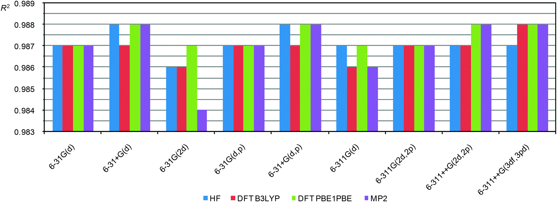Fig. 3 R ² values (PBE1PBE/6-31G(d) level for CS calculations) against the indicated functional/basis set approach used in geometry optimization of 23 representative molecules.

Variation of the method to calculate shielding constants. The next step involved the attempt to see how the method used to calculate CSs influences their quality. Similar as above, three fixed sets of geometries for 23 model compounds (optimized at PBE1PBE/6-31G(d), PBE1PBE/6-31+G(d,p) and PBE1PBE/6-311++G(2d,2p) levels) were used. In frames of each set, the CSs were calculated at HF, DFT and MP2 levels. Basis sets were varied in a wide range (Tables S3–S5, ESI†). In addition, the influence of the functional type was also probed. For example, in Fig. 4 the R² data for PBE1PBE/6-31G(d) optimized geometries are shown (data for models optimized in frames of more heavier basis sets are given in the ESI†).

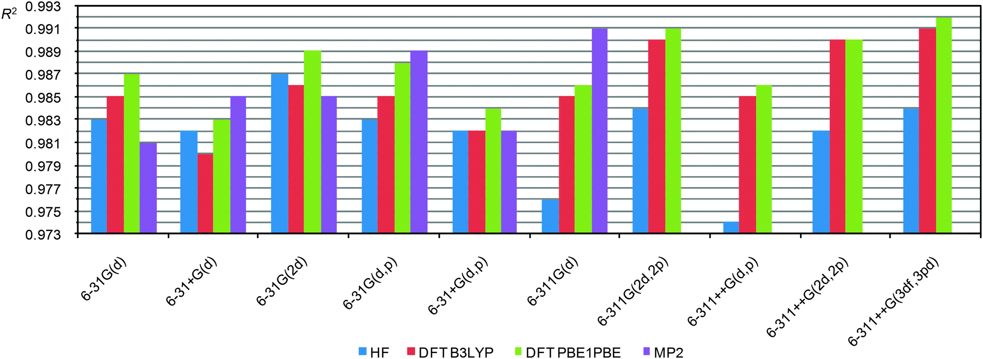Fig. 4 R ² values (the geometry optimized at the PBE1PBE/6-31G(d) level) against the indicated functional/basis set approach used in CS calculations of 23 representative molecules.

As one can see, in this case the R² depends more strongly on the level of theory, on the quality of the basis sets and even on the functional. All three sets (for all basis sets used for geometry optimization) demonstrate similar dependencies. Analysis of these data allows us to reveal key factors that influence the correlation coefficients. First, the inclusion of additional diffuse functions makes the correlation worse. Second, the inclusion of additional polarization functions on heavy atoms (2d) or protons (p) augments the correlation. Third, MP2 calculations in some cases (6-31G(d,p) and 6-311G(d)) improve correlations (the MP2 calculations were possible to run only up to the 6-311G(d) basis set. Heavier basis sets become impractical even for small compounds, vide infra). Fourth, the use of triple split valence basis sets in conjunction with additional polarization functions (6-311G(2d,2p) or 6-311++G(3df,3pd)) improve the correlation coefficient, thus R² becomes similar to the value obtained from MP2 calculations using moderately heavy basis sets (6-31G(d,p) and 6-311G(d)).

From these data it looks like the PBE1PBE functional is superior than B3LYP for CS calculations. But perhaps this might be due to the fact that B3LYP CS calculations were carried out on geometry optimized by the PBE1PBE functional and not by B3LYP, i.e. due to not using a “parent” functional (different for optimization and CS calculations). To prove or disprove this hypothesis we carried out a correlation analysis for the data obtained using the B3LYP functional for both the CS calculations and geometry optimization as well (using the 6-31G(d) basis set). In this case the R² (B3LYP/6-31G(d)//B3LYP/6-31G(d)) = 0.982 that is clearly lower than the correlation for PBE1PBE/6-31G(d)//PBE1PBE/6-31G(d) (R² = 0.987) and even for the B3LYP/6-31G(d)//PBE1PBE/6-31G(d) combinations (R² = 0.985). Thus, the PBE1PBE functional indeed is preferable to use particularly at the CS calculation step.

It is also important that DFT (PBE1PBE) calculations, particularly using heavy basis sets, result in good R² values which are close to MP2 results. The HF level gives a correlation similar to DFT results when small basis sets are used. However, using triple split valence basis sets HF calculations of CS are notably worse.

Thus, CS calculations at the PBE1PBE/6-31G(d) level are good enough. Inclusion of additional polarization functions should improve the correlation. A notable improvement is observed for heavy basis sets, like 6-311G(2d,2p) or 6-311++G(3df,3pd).

At the same time it is necessary to stress that for most of the “combinations” slopes of linear approximation lines are not equal to 1, and these lines do not cross the co-ordinate origin (e.g. for selected combinations, see Table 1), i.e. calculations suffer from disadvantage due to systematic errors. This sort of disagreement is easily eliminated via linear scaling. But before the phase-state problem and the question of correct reference have to be considered which may also be concerned with the above limitations.

Calculation costs and optimal combination

In order to reach a final conclusion about optimal combination that can be used in practice for middle–large size compounds it is necessary to estimate time expenditures. Thus, herewith we analyze the computational costs for the geometry optimization and for CS calculations of middle-size compounds of our test list (vide infra), e.g. 1,2-bis(2,4,5-tri-tert-butyl-diphospholyl) ethane (35) (Fig. 5 and Table S6, ESI†). In general, the geometry optimization step is the most time consuming (Table S6, ESI†), therefore the MP2 approach can hardly be recommended for geometry optimization because its use dramatically increases the computational time (e.g. data for small compound 5 are given in Table S7, ESI†). It becomes practically unaffordable for middle-size compounds, and what is more, it does not improve the correlation with respect to other methods. DFT calculations with relatively simple basis sets (6-31G(d) or 6-31+G(d)) are expected to give good results. Further augmentation of the basis set leads to only insignificant improvement, while time costs increase dramatically (Fig. 5a). The HF level is least time consuming (Table S7, ESI†) and gives reasonably good geometry, and therefore can be recommended for geometry optimization of large compounds for which the DFT method is inapplicable.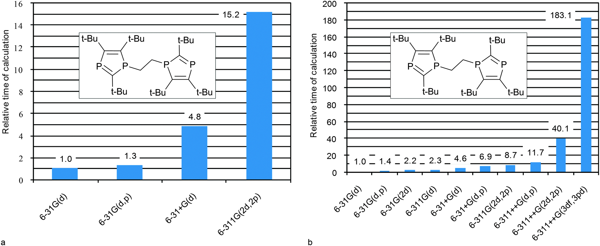

Fig. 5 Relative computational costs against the indicated basis set approach (at DFT PBE1PBE level of theory) used at geometry optimization (a) and CSs calculations (b) for 35.

The CS calculation step being less time consuming, heavier basis sets can be easily applied. The PBE1PBE/6-31G(2d) level for CS calculations is a good compromise between the cost and the quality. If one needs more accurate data, the 6-311G(2d,2p) basis set can be recommended since such calculations are still affordable. Further augmentation of the basis set only leads to an unreasonable increase of computational costs (Fig. 5b).

To sum it up the PBE1PBE/6-31G(d)//PBE1PBE/6-31G(d) level can be recommended for express estimation of ³¹P CS. The PBE1PBE/6-31G(2d)//PBE1PBE/6-31G(d) combination can be recommended for routine applications. The PBE1PBE/6-311G(2d,2p)//PBE1PBE/6-31+G(d) level should be used to obtain better results at a reasonable cost (Table 1). If one deals with a very large molecule, PBE1PBE/6-311G(2d,2p)//HF/6-31G(d) can be recommended as a compromise.

Phase state problem

Theoretically calculated NMR shielding values must be compared with experimental values determined in the gas phase. However, the amount of such data is very limited. On the other hand, what is more interesting for NMR spectroscopists is the possibility of carrying out the calculations of CSs determined in solution. Therefore, the question arises: is it correct to compare CSs calculated in the gas phase with experimental CS NMR data obtained in solution?

In order to answer this question, let us consider in detail the possible contributions to shielding in media. In general, the shielding of a particular atom in the environment can be written in the following form:

σ = σ_vacuum + σ_dia + σ_polar + σ_rovibrat + σ_{specific solvent effect} (1)

where σ_vacuum is the magnetic shielding for an isolated molecule in vacuum, σ_dia is the contribution of the bulk diamagnetic susceptibility of the sample, σ_polar is the impact of the medium polarity, σ_rovibrat is a rovibronic correlation term, and σ_{specific solvent effect} is the impact of specific solvent effects.

And CS is determined according to eqn (2):

δ(X) = σ(stand) − σ(X) + δ(stand) (2)

where the shielding of the molecule of interest (X) and the standard should be measured under identical conditions.

The second term in eqn (1) arises because the magnetic field in solution is different from the one in vacuum. However, this term for the most common solvents is small (0.3–0.8 ppm). Moreover, it is nearly the same both for the molecule X and for the standard and, therefore, its contribution to the CS can be neglected.

The third term in eqn (1) accounts for the influence of the solvent’s polarity on the electron density distribution. From this point of view it can be expected that more polar molecules can be more sensitive to these effects than the less polar ones. In order to estimate the magnitude of the possible contribution due to the polarity of the solvent, one can try to calculate this contribution theoretically and measure experimentally.⁴⁹

According to calculations in frames of the polarizable continuum model (PCM)⁸⁰ for several model compounds (H₃PO₄ (4, 0.02 D), P(OEt)₃ (36, 1.50 D), (CH₃)₃PO (7, 4.32 D)), the magnetic shielding difference in vacuum and in benzene (ε = 2.3) should be negligible (less than 0.7 ppm) for non-polar molecules (Table S8, ESI†). Only for a relatively polar molecule ((CH₃)₃PO (4.32 D)), this contribution may be notable (up to 7 ppm). According to the calculations, the increase of solvent’s polarity (e.g. ε (CHCl₃) = 4.7) should not change the shielding significantly (Table S8, ESI†).

On the other hand, at a fixed magnetic field, the changes in CSs of compounds P(OEt)₃ (36), HP(O)(OEt)₂ (37) and ClP(O)(OEt)₂ (38) do not exceed 0.8 ppm upon the transition from non-polar (C₆H₆, ε = 2.3) to moderately polar (CHCl₃, ε = 4.7) solvents (Table S8, ESI†). Thus, the contribution of the polarity of the medium to phosphorus shielding is also insignificant and should not exceed 7 ppm. Therefore, the dependence of CS on the polarity should be even less and may be neglected in quantum-chemical calculations.

The next is the rovibrational term in eqn (1), which is not taken into account in quantum chemical calculations. According to estimations, this term is also small (less than 10 ppm)⁸¹ and if to take into account that there is a similar contribution to the shielding of the standard, the impact of this term in CS should also be small.

The most ambiguous is the situation with the last term in eqn (1) which reflects the contributions from specific intermolecular interactions. The experimentally measured CSs correspond to the thermodynamic ensemble of molecules interacting with each other and/or with the solvent molecules. In most cases, the interactions are weak dispersion ones of the title and solvent molecules, and the gas phase approximation is correct. A different situation may occur in the presence of specific intermolecular interactions. In these cases, the changes in geometry (due to association, self-association, tautomeric or conformational transformations) can be significant and may influence CSs notably, so that the calculated and experiment data can dramatically disagree. In such cases, in order to verify the absence of significant effects of intermolecular interactions and self-association on CSs, it is necessary to examine the concentration dependence of the CSs or solvent dependence (polar/nonpolar). In each such case, it should be considered individually.

Thus, if there are no specific interactions, the calculated CSs for vacuum should well reproduce experimental values.

Problem of the right choice of reference

Today, the accepted reference standard for ³¹P NMR spectroscopy is 85% water solution of H₃PO₄. However, there is no value for it in the gas phase that makes difficult the use of this compound as a reference in the calculations. The situation seems to be even more problematic, if to take into account that the real standard is a highly concentrated compound with functional groups prone to strong specific hydrogen bonding. In addition, water is a very polar solvent that may also be involved in association with H₃PO₄ molecules.⁵⁹ Therefore, strong medium effects can be expected for this standard. As a result, the isolated molecule approximation may not be valid in calculations for this compound.

Alternatively, the secondary reference like PH₃ is often used because its value in the gas phase is documented. But, in fact, its ³¹P CS strongly depends on the phase state as well (−266.1 and −238 ppm in the gas and the neat liquid, respectively)⁴⁸ implicating notable association effects in solution. In other words, PH₃ is also not a good reference. Thus, in fact, both references widely used in calculations, are not perfect.

However, to our opinion, in fact there is no need to refer exclusively to the gas phase data. After all, if one tries to be fully correct and refer to the standard in the gas phase, the results of calculations for the compound of interest should also be compared only with its gas phase data, which is impossible in most of the cases.

On the other hand, for most “normal” systems referencing relative to the generally accepted standard H₃PO₄ gives CSs, which can be compared with experimental data obtained in solution. That is, the calculated data correlate well the experiment carried out in solution with some under- or over-estimation (depending on the “combination” used). As a last resort, the empirical correction can be applied to overcome this problem.

Linear Scaling

Linear scaling allows the improvement of the calculated CSs via linear regression of the calculated CSs versus experimental data.^82–85 The linear regression method is capable of correcting systematic errors across the whole ³¹P NMR spectra. As a result, the slope and the intercept from the best-fit line allow for the calculation of the empirically scaled CSs according to eqn (3)

δ_scaled = (δ_unscaled − intercept)/slope (3)

where δ_unscaled is the calculated CS for a particular nucleus. Thus, in eqn (3), the intercept helps to correct the error for a reference compound while the slope provides information about the size of the systematic error.§ This operation has been carried out for each of the four “combinations”, and the root-mean-square errors (RMSEs) relating the scaled CS predictions with experiment appear in the bottom row of Table 1. While not small enough as one might like, RMSE = 10.9 ppm for the best “combination” nonetheless indicates that DFT calculations of ³¹P CSs, followed by linear scaling, provide a chemically useful degree of accuracy. The procedure that we recommend as the “express method” (PBE1PBE/6-31G(d)//PBE1PBE/6-31G(d)) yields a slightly greater RMSE = 14.6 ppm than the PBE1PBE/6-311G(2d,2p)//PBE1PBE/6-31+G(d) combination which gives the best compromise between accuracy and economy.

It is interesting to note that the scaled CSs for the frequently used secondary reference, PH₃, agree better with its experimental value in liquid than in the gas phase implying that referencing to its gas phase would produce worse CSs for the whole set of model compounds.

“Difficult” cases

At the beginning of the analysis we found that there are some “exceptions” for which the difference between experimental and calculated data was essential regardless of the level of theory used. These are PN (30), P₂H₂ (26), [PCl₆]⁻ (22), [PF₆]⁻ (21), FCP (28), (CH₃PCl₂) (23), (CH₃O)₃PS (33), P(SCH₃)₃ (34), PCl₃ (24) and H₃PO (1). Some of these “exceptions” (PN, P₂H₂, PCl₃, [PCl₆]⁻, [PF₆]⁻) were already discussed in the literature.^38,48,86

In general, the reasons for such discrepancies may be divided into two types: the drawback of theoretical models and the interference of additional medium effects in a real experiment that is not accounted for. For example, it was supposed that the disagreement between experimental and calculated ³¹P CSs for PCl₃ and PN might be due to the inadequate description of their structures at the DFT level. Therefore if to take into account that the paramagnetic contribution to the magnetic shielding in these molecules is large, CS will strongly depend on the bond lengths.⁴⁷

On the other hand, relativistic effects arising from magnetic shielding of the nucleus located in the vicinity of the atoms of third period elements may also be strong.^5,51,54 The relativistic spin–orbital interaction is not accounted for in our calculations and therefore the problems for (CH₃)₃PS and P(SCH₃)₃ might be well due to the contribution from relativistic effects of vicinal sulfur atoms. The same reason may account for the discrepancy observed for PCl₃.

Some of the above “exceptions” may be due to the “incorrect” description of the molecular system in calculations. Namely, if molecules in solution are prone to association or self-association, the isolated molecular model will not be correct.^53,55 Intra- or intermolecular coordination involving phosphorus results in a dramatic ³¹P nuclear shielding amounting to approximately 150 ppm upon changing the phosphorus coordination number by one.⁵⁵ Thus, the impact of associated forms in solution may dramatically change the observed ³¹P CSs.

For example, the accurate prediction of ³¹P NMR CSs of ion pair systems requires consideration of the full system.⁴⁹ Therefore, the deviations observed for the small ions, [PCl₆]⁻ and [PF₆]⁻, presumably, are due to considerable solvent or counterion effects.⁴⁸

In a similar way, intermolecular coordination may be responsible for the discrepancies observed for PN, P₂H₂ and FCP. In solution these molecules may exist not only in a monomolecular form but also in the associated form, as well. The calculations performed for the (PN)₃ complex in fact demonstrate that, on the one hand, the trimer is much more stable than the monomer. On the other hand, while theoretical CSs (PBE1PBE/6-31G(d)//PBE1PBE/6-31G(d)) of the monomer deviates to the lower field (336.4 ppm) from the experimentally observed one (275.0 ppm), the value of the trimer shifts in the opposite direction (262.1 ppm). Thus, the experimental value lies somewhere in between these calculated values for two structural forms, i.e. calculated and experimental CSs agree if one supposes that there is a fast exchange between these forms. Similar considerations can also be applied to P₂H₂ and FCP molecules as well.

Another reason for the discrepancy to occur may be due to the system that is involved in intramolecular exchange processes. In this case consideration of only one form may not be enough. For example, the calculations performed for phosphine oxide (H₃P=O, 1a) underestimate the ³¹P CS by ca. 36 ppm (Fig. 6). However, if to suppose that this form is in exchange with the acid tautomer^58,87–95 the contradiction will be resolved.

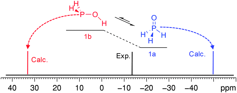Fig. 6 Equilibrium of phosphine oxide (1a) and phosphinous acid (1b) and schematical representation of ³¹P spectra of 1.

According to the calculations, these two forms are close in energy in vacuum (Table S9, ESI†). In H₂O solution, e.g. in the frame of PCM, the preference is expected to invert although the energy gap is still small (Table S9, ESI†), i.e. the populations of these two forms should be close or comparable. Further on, if to take into account that the calculation for phosphinous acid (1b) predicts the ³¹P CS at a notably lower field (ca. 34 ppm), the experimental value corresponds to the intermediate between these tautomeric forms which may be in fast exchange in the NMR time scale (Fig. 6).

This hypothesis is also strongly supported by the finding that a similar pentafluorophenyl derivative in solution exists in equilibrium with the phosphinous acid (C₆F₅(C₂F₅)POH, 39a) and phosphane oxide (C₆F₅(C₂F₅)P(O)H, 39b) tautomers.⁹⁶ Due to higher barrier of exchange in this case both tautomers are observed separately in ³¹P NMR spectra (80.6 and −1.9 ppm, respectively). To this end, the calculations using PBE1PBE/6-31G(d)//PBE1PBE/6-31G(d) for the pentafluorophenyl derivative predicts that ³¹P CSs are in good agreement with experiment (71.4 and −10.8 ppm for acid and oxide tautomers, respectively).

In the case of other acids (e.g. H₃PO₂ (2), H₃PO₃ (3)) no deviations from experiment were observed suggesting a strong preference to one tautomeric form (Table S9, ESI†). Energy analysis for these acids also supports this conclusion, viz. there is an essential preference to one dominant form and solvent has only an insignificant effect on the energy gap. Thus, in solution these acids are in one form and calculations well describe their NMR CSs.

The second question – will the required level of theory (established for small models) work well “for larger organophosphorus compounds of practical interest”? And will it be within the limits of computational resources? To answer these questions typical representatives of several classes of phosphorus compounds with a molecular weight of about 200–300 Da (Fig. 7) were analyzed. Calculations were run on PBE1PBE/6-311G(2d,2p)//PBE1PBE/6-31+G(d), PBE1PBE/6-31G(2d)//PBE1PBE/6-31G(d) and PBE1PBE/6-31G(d)//PBE1PBE/6-31G(d) levels of theory. A linear scaling procedure was applied to GIAO calculated CSs (Table S10, ESI†).

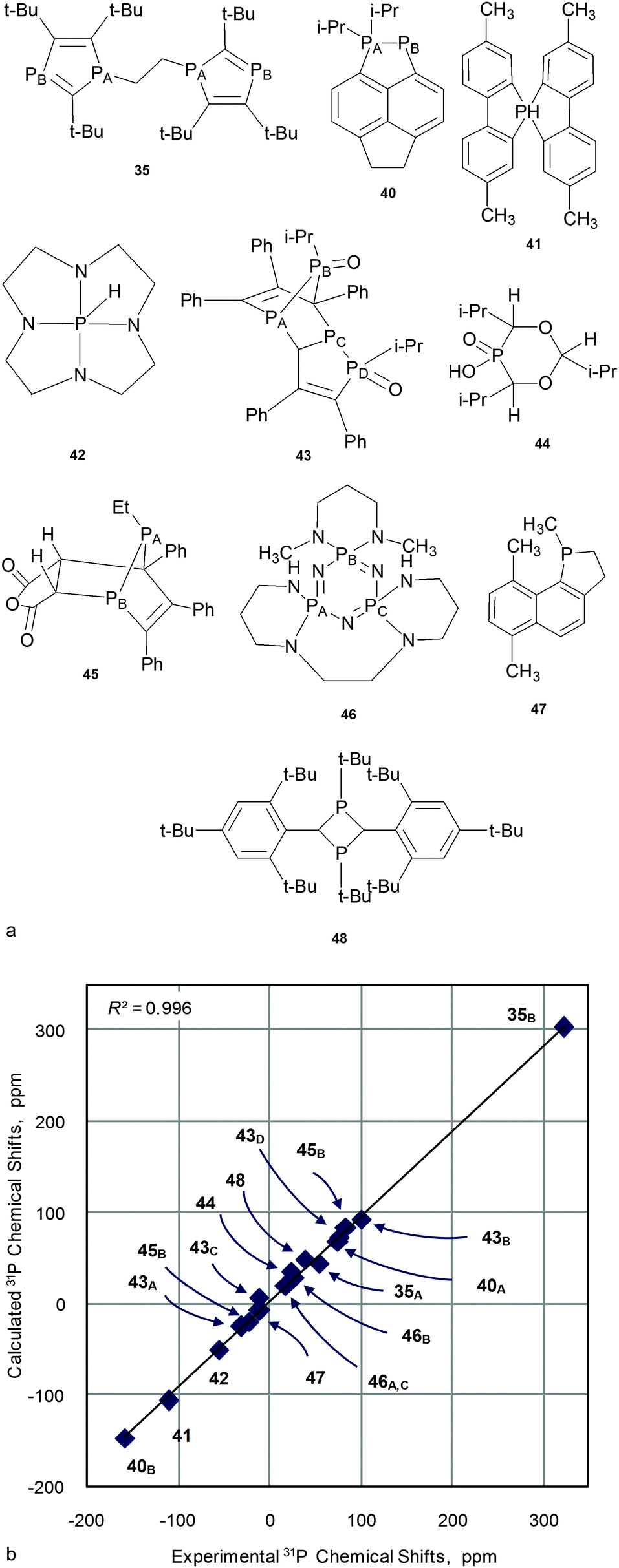Fig. 7 Structures of “large compounds” 35, 40–48 (a) and the correlation of experimental versus calculated at PBE1PBE/6-311G(2d,2p)//PBE1PBE/6-31+G(d) ³¹P NMR CS for 35, 40–48 (b).

On the whole, calculated values agree well with experimental data for all combinations tested (e.g. for the PBE1PBE/6-311G(2d,2p)//PBE1PBE/6-31+G(d) combination, see Fig. 7 and Table 2; for the rest, see Table S10, ESI†). In all cases correlations are close to linearity (R² = 0.989–0.996) and RMSE are small (9.0–11.6 ppm).

Table 2 Calculated^a and experimental ³¹P NMR CSs for 35, 40–48

No.	δ unscaled	δ scaled	δ exp	Solvent	Ref.
a At the PBE1PBE/6-311G(2d,2p)//PBE1PBE/6-31+G(d) level. b In ppm. c Not available.
35	32.1	43.3	54.8	C6H6	97
	309.6	302.0	322.9
40	−172.4	−147.3	−157.7	na^c	98
	63.9	72.9	76.7
41	−129.3	−107.2	−110.0	na	99
42	−68.6	−50.5	−54.5	na	100
43	−41.9	−25.7	−29.7	CHCl3	101
	84.1	91.7	100.5
	−7.1	6.7	−10.6
	58.7	68.1	75.7
44	22.5	34.3	24	C6H6	102
45	74.3	82.6	84.1	CHCl3	103
	−36.5	−20.6	−22.6
46	15.0	27.4	27.6	CHCl3	104
	5.8	18.8	18.3
47	−23.1	−8.1	−10.2	CHCl3	105
48	36.8	47.7	38.7	CHCl3	106
R ^2	0.996	0.996
RMSE (ppm)		9.0

---

Application of ³¹P NMR CSs to isomeric structure determination

Being very sensitive to the chemical structure, the ¹³C and ¹⁵N CSs can be safely used to establish fine structural features such as isomerism and tautomerism.^16–35 The ³¹P CS is even more sensitive to structural modifications and, perhaps, could also be used to analyze the features of geometry of phosphorus containing compounds. To check this idea, we used 10-ethyl-7,8,9-triphenyl-4-oxa-1,10-diphospatricyclo[5.2.1.02,6]-deca-8-ene-3,5-dione (45) for which several isomeric forms can be realized and for which reliable structural data are available¹⁰³ as obtained by an alternative method. Thus, we run the CS calculations for four isomers of 45 (Fig. 8a) and compared with experimental data for both phosphorus atoms (Table S11, ESI†).

Fig. 8 Possible structural isomers of 45 (a) and Δδ = δ_calc − δ_exp for isomers of 45 (b). Calculations at PBE1PBE/6-311G(2d,2p)//PBE1PBE/6-31+G(d) level of theory.

According to the calculations, the ³¹P CSs essentially depend on the isomeric structure varying within 100 ppm (Table S11, ESI†). However, only in the case of the A isomer, the differences between theoretical and experimental ³¹P CSs are small (less than 3 ppm) while in other cases deviations are high (Fig. 8b). Thus the analysis of ³¹P CSs allows a simple and unequivocal assignment of the isomeric form of 45 to structure A that is in full agreement with X-ray data.¹⁰³

Conclusions

A comparative analysis of calculated (GIAO) versus experimental ³¹P NMR CSs for a wide range of organophosphorus model compounds was carried out. A variety of combinations (levels of theory (HF, DFT, and MP2), functionals (B3LYP and PBE1PBE) and basis sets (6-31G(d), 6-31+G(d), 6-31G(2d), 6-31G(d,p), 6-31+G(d,p), 6-311G(d), 6-311G(2d,2p), 6-311++G(d,p), 6-311++G(2d,2p), and 6-311++G(3df,3pd))) were tested to reveal main factors that influence the quality of calculated data. On the whole, with the exception of some “difficult” cases (FCP, OPH₃, PN, P₂H₂, PCl₃, [PCl₆]⁻, [PF₆]⁻, (CH₃)₃PS, and P(SCH₃)₃) the calculated ³¹P CSs satisfactorily correlate with experimental data.

To sum it up, the PBE1PBE/6-31G(d)//PBE1PBE/6-31G(d) level can be recommended for express estimation of ³¹P CS of organophosphorus compounds. The PBE1PBE/6-31G(2d)//PBE1PBE/6-31G(d) combination can be recommended for routine applications. The PBE1PBE/6-311G(2d,2p)//PBE1PBE/6-31+G(d) level can be proposed to obtain better results at a reasonable cost. In the case of very large molecules PBE1PBE/6-311G(2d,2p)//HF/6-31G(d) can be recommended as a compromise. Scaling by linear regression parameters significantly improves results.

Care has to be taken for compounds that may be involved in exchange between different structural forms (self-associates, associates with solvent, tautomers, and conformers) and therefore, experimental ³¹P CSs may correspond to the exchange averaged values. In such suspicious cases the disagreement between calculated and experimental data most likely “says” that the problem formulation is incorrect.

Problems for phosphorus located near the atoms of third period elements ((CH₃)₃PS and P(SCH₃)₃) may be due to the impact of relativistic effects that was not accounted for in our calculations.

³¹P CSs can be safely used to establish fine structural peculiarities such as isomeric and tautomeric structures.

Experimental part

All of the calculations were performed using the Gaussian 03 program.¹⁰⁷ A PC with Core i7-3960x CPU, 16 GB RAM with 64× Windows 7 operating system was used. NMR experiments were performed using a Bruker AVANCE-500 spectrometer (11.7 T) at 303 K. ³¹P spectra were acquired at a fixed magnetic field and referenced to external H₃PO₄.

Acknowledgements

This study was financially supported in part by the Russian Foundation for Basic Research (Projects 13-03-00169 and 14-03-31952). Dmitry G. Yakhvarov thanks Russian Scientific Fund (project 14-13-01122) for supporting the research activity towards phosphane oxide H₃PO.

References

1. F. Blanco, I. Alkorta and J. Elguero, Magn. Reson. Chem., 2007, 45, 797.
2. A. Bagno, F. Rastrelli and G. Saielli, J. Org. Chem., 2007, 72, 7373.
3. S. Rosselli, M. Bruno, A. Maggio, G. Bellone, C. Formisano, C. A. Mattia, S. Di Micco and G. Bifulco, Eur. J. Org. Chem., 2007, 2504.
4. G. Bifulco, R. Riccio, C. Gaeta and P. Neri, Chem. – Eur. J., 2007, 13, 7185.
5. A. Balandina, A. Kalinin, V. Mamedov, B. Figadère and Sh. Latypov, Magn. Reson. Chem., 2005, 43, 816.
6. R. M. Claramunt, C. Lopez, M. D. Santa Maria, D. Sanz and J. Elguero, Prog. Nucl. Magn. Reson. Spectrosc., 2006, 49, 169.
7. A. R. Katritzky, N. G. Akhmedov, J. Doskocz, P. P. Mohapatra, C. D. Hall and A. Güuven, Magn. Reson. Chem., 2007, 45, 532.
8. D. Sanz, R. M. Claramunt, A. Saini, V. Kumar, R. Aggarwal, S. P. Singh, I. Alkorta and J. Elguero, Magn. Reson. Chem., 2007, 45, 513.
9. A. R. Katritzky, N. G. Akhmedov, J. Doskocz, C. D. Hall, R. G. Akhmedova and S. Majumder, Magn. Reson. Chem., 2007, 45, 5.
10. G. Barone, L. Gomez-Paloma, D. Duca, A. Silvestri, R. Riccio and G. Bifulco, Chem. – Eur. J., 2002, 8, 3233.
11. G. Barone, D. Duca, A. Silvestri, L. Gomez-Paloma, R. Riccio and G. Bifulco, Chem. – Eur. J., 2002, 8, 3240.
12. P. Cimino, L. Gomez-Paloma, D. Duca, R. Riccio and G. Bifulco, Magn. Reson. Chem., 2004, 42, S26.
13. I. Alkorta and J. Elguero, Tetrahedron Lett., 2006, 62, 8683.
14. A. B. Sebag, R. N. Hanson, D. A. Forsyth and C. Y. Lee, Magn. Reson. Chem., 2003, 41, 246.
15. E. Kleinpeter, S. Klod and W.-D. Rudorf, J. Org. Chem., 2004, 69, 4317.
16. Sh. Latypov, A. Balandina, M. Boccalini, A. Matteucci, K. Usachev and S. Chimichi, Eur. J. Org. Chem., 2008, 4640.
17. A. Kozlov, V. Semenov, A. Mikhailov, A. Aganov, M. Smith, V. Reznik and Sh. Latypov, J. Phys. Chem. B, 2008, 112, 3259.
18. A. E. Aliev, Z. A. Mia, M. J. M. Busson, R. J. Fitzmaurice and S. Caddick, J. Org. Chem., 2012, 77, 6290.
19. B. S. Dyson, J. W. Burton, T. Sohn, B. Kim, H. Bae and D. Kim, J. Am. Chem. Soc., 2012, 134, 11781.
20. R. Pohl, F. Potmischil, M. Dračínský, V. Vaněk, L. Slavětínská and M. Buděšínský, Magn. Reson. Chem., 2012, 50, 415.
21. M. W. Lodewyk, M. R. Siebert and D. J. Tantillo, Chem. Rev., 2012, 112, 1839.
22. M. G. Chini, C. R. Jones, A. Zampella, M. V. D’Auria, B. Renga, S. Fiorucci, C. P. Butts and G. Bifulco, J. Org. Chem., 2012, 77, 1489.
23. G. Saielli, K. C. Nicolaou, A. Ortiz, H. Zhang and A. Bagno, J. Am. Chem. Soc., 2011, 133, 6072.
24. S. G. Smith and J. M. Goodman, J. Am. Chem. Soc., 2010, 132, 12946.
25. F. A. A. Muldera and M. Filatov, Chem. Soc. Rev., 2010, 39, 578.
26. S. G. Smith and J. M. Goodman, J. Org. Chem., 2009, 74, 4597.
27. A. M. Belostotskii, J. Org. Chem., 2008, 73, 5723.
28. G. Bifulco, P. Dambruoso, L. Gomez-Paloma and R. Riccio, Chem. Rev., 2007, 107, 3744.
29. M. J. Bartlett, P. T. Northcote, M. Lein and J. E. Harvey, J. Org. Chem., 2014, 79, 752.
30. S. Di Micco, M. G. Chini, R. Riccio and G. Bifulco, Eur. J. Org. Chem., 2010, 1411.
31. S. G. Smith and J. M. Goodman, J. Org. Chem., 2009, 74, 4597.
32. F. F. Fleming and G. Wei, J. Org. Chem., 2009, 74, 3551.
33. B. Vera, A. D. Rodriguez, E. Aviles and Y. Ishikawa, Eur. J. Org. Chem., 2009, 5327.
34. A. Balandina, V. Mamedov, X. Franck, B. Figadere and Sh. Latypov, Tetrahedron Lett., 2004, 45, 4003.
35. S. Chimichi, M. Boccalini, A. Matteucci, S. V. Kharlamov, Sh. K. Latypov and O. G. Sinyashin, Magn. Reson. Chem., 2010, 48, 607.
36. J. G. Verkade and L. D. Quin, Methods in Stereochemical Analysis Volumes in the Series: Phosphorus 31 NMR Spectroscopy in Stereochemical Analysis, VCH Publishers, Deerfield Beach, Florida, 1987.
37. T. M. Alam, Int. J. Mol. Sci., 2002, 3, 888.
38. I. Alkorta and J. Elguero, Struct. Chem., 1998, 9, 187.
39. K. Chruszcza, M. Barańska, K. Czarnieckia, B. Boduszek and L. M. Proniewicz, J. Mol. Struct., 2003, 648, 215.
40. P. Mroz, Mol. Phys. Rep., 2000, 29, 208.
41. I. S. Koo, D. Ali, K. Yang, Y. Park, D. M. Wardlaw and E. Buncel, Bull. Korean Chem. Soc., 2008, 29, 2252.
42. Y. Ruiz-Morales and T. Ziegler, J. Phys. Chem. A, 1998, 102, 3970.
43. T. M. Alam, Sandia report, Sandiy National Laboratories Albuquerque, New Mexico 87185 and Livermore, California 94550, 1998.
44. M. Pecul, M. Urbánczyk, A. Wodynskia and M. Jaszúnskib, Magn. Reson. Chem., 2011, 49, 399.
45. L. Benda, Z. Sochorová-Vokáčová, M. Straka and V. Sychrovský, J. Phys. Chem. B, 2012, 116, 3823.
46. M. Rezaei-Sameti, THEOCHEM, 2008, 867, 122.
47. A. B. Rozhenko, W. W. Schoeller and M. I. Povolotskii, Magn. Reson. Chem., 1999, 37, 551.
48. C. van Wüllen, Phys. Chem. Chem. Phys., 2000, 2, 2137.
49. B. Maryasin and H. Zipse, Phys. Chem. Chem. Phys., 2011, 13, 5150.
50. K. A. Chernyshev and L. B. Krivdin, Russ. J. Org. Chem., 2010, 46, 785.
51. K. A. Chernyshev, L. B. Krivdin, S. V. Fedorov, S. N. Arbuzova and N. I. Ivanova, Russ. J. Org. Chem., 2013, 49, 1420.
52. K. A. Chernyshev, L. I. Larina, E. A. Chirkina, V. G. Rozinov and L. B. Krivdin, Russ. J. Org. Chem., 2012, 48, 676.
53. K. A. Chernyshev, L. I. Larina, E. A. Chirkina, V. G. Rozinov and L. B. Krivdin, Russ. J. Org. Chem., 2011, 47, 1865.
54. S. V. Fedorov, Yu. Yu. Rusakov and L. B. Krivdin, Magn. Reson. Chem., 2014, 52, 699.
55. K. A. Chernyshev, L. I. Larina, E. A. Chirkina and L. B. Krivdin, Magn. Reson. Chem., 2012, 50, 120.
56. G. Manca, M. Caporali, A. Ienco, M. Peruzzini and C. Mealli, J. Organomet. Chem., 2014, 760, 177.
57. N. S. Golubev, R. E. Asfin, S. N. Smirnov and P. M. Tolstoi, Russ. J. Gen. Chem., 2006, 76, 915.
58. S. G. Kozlova, S. P. Gabuda and R. Blinc, Chem. Phys. Lett., 2003, 376, 364.
59. D. B. Chesnut, J. Phys. Chem. A, 2005, 109, 11962.
60. L. Z. Maier, Z. Anorg. Allg. Chem., 1972, 394, 117.
61. G. Haegele, W. Kuchen and H. Steinberger, Z. Naturforsch., B: Anorg. Chem., Org. Chem., 1974, 29, 349.
62. H. H. Karsch, Phosphorus, Sulfur Silicon Relat. Elem., 1982, 12, 217.
63. F. Seel and H. J. Bassler, Z. Anorg. Allg. Chem., 1976, 423, 67.
64. L. D. Quin and C. E. Roser, J. Org. Chem., 1974, 39, 3423.
65. M. J. Gallagher and H. J. Honegger, J. Chem. Soc., Chem. Commun., 1978, 54.
66. W. Stec, B. Uznanski, D. Houalla and R. Wolf, C. R. Seances Acad. Sci., Ser. C, 1975, 281, 727.
67. N. Zumbulyadis and B. P. Dailey, Mol. Phys., 1974, 27, 633.
68. P. Junkes, M. Baudler, J. Dobbers and D. Rackwitz, Z. Naturforsch., B: Anorg. Chem., Org. Chem., Biochem., Biophys., Biol., 1972, 27, 1451.
69. V. E. Bel’skii, G. V. Romanov, V. M. Pozhidaev and A. N. Pudovik, Zh. Obshch. Khim., 1980, 50, 1222.
70. D. K. Srivastava, L. K. Krannich and C. L. Watkins, Polyhedron, 1988, 7, 2553.
71. L. D. Quin, M. J. Gallagher, G. T. Cunkle and D. B. Chesnut, J. Am. Chem. Soc., 1980, 102, 3136.
72. C. S. Reddy and R. Schmutzler, Z. Naturforsch., B: Anorg. Chem., Org. Chem., Biochem., Biophys., Biol., 1970, 25, 1199.
73. K. B. Dillon and A. W. G. Platt, Phosphorus, Sulfur Silicon Relat. Elem., 1984, 19, 299.
74. L. Maier, Helv. Chim. Acta, 1964, 47, 238.
75. T. D. Bouman and A. E. Hansen, Chem. Phys. Lett., 1990, 175, 292.
76. H. Eshtiagh-Hosseini, H. W. Kroto, J. F. Nixon, S. Brownstein, J. R. Morton and K. F. Preston, J. Chem. Soc., Chem. Commun., 1979, 653.
77. S. P. Anderson, H. Goldwhite, D. Ko, A. Letsou and F. Espraza, J. Chem. Soc., Chem. Commun., 1975, 744.
78. J.-M. Alcaraz and F. Mathey, Tetrahedron Lett., 1984, 25, 4659.
79. L. Maier, Helv. Chim. Acta, 1976, 59, 252.
80. J. Tomasi, R. Bonaccorsi, R. Cammi and F. J. Olivares del Valle, J. Mol. Struct., 1991, 234, 401.
81. P. Lanto, K. Kackowski, W. Makulski, M. Olejniczak and M. Jaszunski, J. Phys. Chem. A, 2011, 115, 10617.
82. P. R. Rablen, S. A. Pearlman and J. Finkbiner, J. Phys. Chem. A, 1999, 103, 7357.
83. R. Jain, T. Bally and P. R. Rablen, J. Org. Chem., 2009, 74, 4017.
84. A. E. Aliev, D. Courtier-Murias and S. Zhou, THEOCHEM, 2009, 893, 1.
85. I. A. Konstantinov and L. J. Broadbelt, J. Phys. Chem. A, 2011, 115, 12364.
86. V. G. Malkin, O. L. Malkina and D. R. Salabub, Chem. Phys. Lett., 1993, 204, 87.
87. F. Wang, P. L. Polavarapu, J. Drabowicz, M. Mikołajczyk and P. Łyzùwa, J. Org. Chem., 2001, 66, 9015.
88. D. B. Chesnut, Heteroat. Chem., 2000, 11, 73.
89. A. Christiansen, C. h. Li, M. Garland, D. Selent, R. Ludwig, A. Spannenberg, W. Baumann, R. Franke and A. Börner, Eur. J. Org. Chem., 2010, 2733.
90. Yu. A. Ustynyuk and Yu. V. Babin, Ross. Khim. Zh., 2007, 51, 130.
91. F. Wang, P. L. Polavarapu, J. Drabowicz and M. Mikołajczyk, J. Org. Chem., 2000, 65, 7561.
92. Y.-L. Zhao, J. W. Flora, W. D. Thweatt, S. L. Garrison, C. Gonzalez, K. N. Houk and M. Marquez, Inorg. Chem., 2009, 48, 1223.
93. M. W. Schmidt, Y. Satoshi and M. S. Gordon, J. Phys. Chem., 1984, 88, 382.
94. S. S. Wesolowski, N. R. Brimkmann, E. F. Valeev, H. F. Schaefer, M. P. Repasky and W. L. Jorgensen, J. Chem. Phys., 2002, 116, 112.
95. D. Yakhvarov, M. Caporali, L. Gonsalvi, Sh. Latypov, V. Mirabello, I. Rizvanov, O. Sinyashin, P. Stoppioni and M. Peruzzini, Angew. Chem., Int. Ed., 2011, 50, 5370.
96. N. Allefeld, M. Grasse, N. Ignat'ev and B. Hoge, Chem. – Eur. J., 2014, 20, 8615.
97. J. Steinbach, P. Binger and M. Regitz, Synthesis, 2003, 2720.
98. B. A. Surgenor, M. Bühl, A. M. Z. Slawin, J. D. Woollins and P. Kilian, Angew. Chem., 2012, 124, 10297.
99. D. Hellwinkel and H.-J. Wilfinger, Phosphorus, Sulfur Silicon Relat. Elem., 1976, 6, 151.
100. J. E. Richman and T. J. Atkins, Tetrahedron Lett., 1978, 45, 4333.
101. A. Zagidullin, Y. Ganushevich, V. Milukov, D. Krivolapov, O. Kataeva, O. Sinyashin and E. Hey-Hawkins, Org. Biomol. Chem., 2012, 10, 5298.
102. T. A. Zyablikova, DSc thesis, IOPC KSC RAS, Kazan, 1999.
103. V. Miluykov, I. Bezkishko, A. Zagidullin, O. Sinyashin, P. Lonnecke and E. Hey-Hawkins, Eur. J. Org. Chem., 2009, 1269.
104. G. Y. Ciftci, E. T. Ecik, T. Yildirim, K. Bilgin, E. Senkuytu, F. Yuksel, Y. Uludag and A. Kilic, Tetrahedron Lett., 2013, 69, 1454.
105. L. D. Quin, K. A. Mesch and W. L. Orton, Phosphorus, Sulfur Silicon Relat. Elem., 1982, 12, 161.
106. M. Yoshifurji, Y. Hirano, G. Schnakenburg, R. Streubel, E. Niecke and S. Ito, Helv. Chim. Acta, 2012, 95, 1723.
107. M. J. Frisch, G. W. Trucks, H. B. Schlegel, G. E. Scuseria, M. A. Robb, J. R. Cheeseman, J. A. Montgomery, Jr., T. Vreven, K. N. Kudin, J. C. Burant, J. M. Millam, S. S. Iyengar, J. Tomasi, V. Barone, B. Mennucci, M. Cossi, G. Scalmani, N. Rega, G. A. Petersson, H. Nakatsuji, M. Hada, M. Ehara, K. Toyota, R. Fukuda, J. Hasegawa, M. Ishida, T. Nakajima, Y. Honda, O. Kitao, H. Nakai, M. Klene, X. Li, J. E. Knox, H. P. Hratchian, J. B. Cross, C. Adamo, J. Jaramillo, R. Gomperts, R. E. Stratmann, O. Yazyev, A. J. Austin, R. Cammi, C. Pomelli, J. W. Ochterski, P. Y. Ayala, K. Morokuma, G. A. Voth, P. Salvador, J. J. Dannenberg, V. G. Zakrzewski, S. Dapprich, A. D. Daniels, M. C. Strain, O. Farkas, D. K. Malick, A. D. Rabuck, K. Raghavachari, J. B. Foresman, J. V. Ortiz, Q. Cui, A. G. Baboul, S. Clifford, J. Cioslowski, B. B. Stefanov, G. Liu, A. Liashenko, P. Piskorz, I. Komaromi, R. L. Martin, D. J. Fox, T. Keith, M. A. Al-Laham, C. Y. Peng, A. Nanayakkara, M. Challacombe, P. M. W. Gill, B. Johnson, W. Chen, M. W. Wong, C. Gonzalez and J. A. Pople, Gaussian 03, Revision A.1, Gaussian, Inc., Pittsburgh PA, 2003.

---

Footnotes

† Electronic supplementary information (ESI) available. See DOI: 10.1039/c5cp00240k

‡ Here and further in the text “higher level of theory” means either higher level (HF–DFT–MP2) and/or more reach basis set. “Heavy combination” means level of theory used either for optimization of geometry or for chemical shift calculation steps.

§ Parameters of the linear scaling equation for different calculation levels are given in the ESI.†

---