
 Open Access Article
 This Open Access Article is licensed under a
 Creative Commons Attribution 3.0 Unported Licence
Activation of C–H and B–H bonds through agostic bonding: an ELF/QTAIM insight†
Emilie-Laure
Zins
ab,
Bernard
Silvi
cd and
M. Esmaïl
Alikhani
*ab
aSorbonne Universités, UPMC Univ. Paris 06, MONARIS, UMR 8233, Université Pierre et Marie Curie, 4 Place Jussieu, case courrier 49, F-75252 Paris Cedex 05, France. E-mail: esmail.alikhani@upmc.fr
bCNRS, MONARIS, UMR 8233, Université Pierre et Marie Curie, 4 Place Jussieu, case courrier 49, F-75252 Paris Cedex 05, France
cSorbonne Universités, UPMC Univ. Paris 06, Laboratoire de Chimie Théorique (LCT), UMR 7616, Université Pierre et Marie Curie, 4 place Jussieu, case courrier 137, F-75252 Paris Cedex 05, France
dCNRS, Laboratoire de Chimie Théorique (LCT), UMR7616, Université Pierre et Marie Curie, 4 place Jussieu, case courrier 137, F-75252 Paris Cedex 05, France
First published on 25th February 2015
Abstract
Agostic bonding is of paramount importance in C–H bond activation processes. The reactivity of the σ C–H bond thus activated will depend on the nature of the metallic center, the nature of the ligand involved in the interaction and co-ligands, as well as on geometric parameters. Because of their importance in organometallic chemistry, a qualitative classification of agostic bonding could be very much helpful. Herein we propose descriptors of the agostic character of bonding based on the electron localization function (ELF) and Quantum Theory of Atoms in Molecules (QTAIM) topological analysis. A set of 31 metallic complexes taken, or derived, from the literature was chosen to illustrate our methodology. First, some criteria should prove that an interaction between a metallic center and a σ X–H bond can indeed be described as “agostic” bonding. Then, the contribution of the metallic center in the protonated agostic basin, in the ELF topological description, may be used to evaluate the agostic character of bonding. A σ X–H bond is in agostic interaction with a metal center when the protonated X–H basin is a trisynaptic basin with a metal contribution strictly larger than the numerical uncertainty, i.e. 0.01 e. In addition, it was shown that the weakening of the electron density at the X–Hagostic bond critical point with respect to that of X–Hfree well correlates with the lengthening of the agostic X–H bond distance as well as with the shift of the vibrational frequency associated with the νX–H stretching mode. Furthermore, the use of a normalized parameter that takes into account the total population of the protonated basin, allows the comparison of the agostic character of bonding involved in different complexes.
I. Introduction
In the context of catalytic processes, understanding the molecular mechanism involving transition metals is of paramount importance. Indeed, since the pioneering studies of Chatt and Davidson1 on one hand, and Bergman2 and Jones3 on the other hand, a considerable number of investigations have demonstrated that transition metal complexes may be involved in C–H bond activation. A thorough study of structures and reactivity of alkyl transition metal complexes has led to the introduction of a new concept: the term “agostic” was proposed to characterize the formation of a 3 center–2 electron (3c–2e) interaction leading to the activation of a C–H bond around transition metal centers.4–7 The choice of a specific term to underline the importance of the activation of the C–H bond proved to be remarkably appropriate. Indeed, thorough investigation of various catalytic processes further lead to the development of numerous reactions involving agostic interactions, such as the alkane oxidative addition,8 C–H bond elimination,9 transcyclometallation,10 cyclometallation of benzoquinoline,11 and Ziegler–Natta polymerization.12,13 In processes such as cyclometallation using d-block transition metals, it was proposed that agostic interactions may play a decisive role. Indeed, these interactions may either favor or prevent some cyclometallations.14A mechanistic study has shown how agostic bonding may lead to deactivation processes of the Grubb catalyst.15 Thus, a thorough understanding of the agostic bonding may help in designing new reagents that may react in a specific way.Despite its paramount importance in catalytic processes, the identification of an agostic interaction is far from obvious. Indeed, even if some approaches were proposed to experimentally or theoretically characterize these 3c–2e interactions, a consensual tool that may qualitatively describe the strength of every kind of agostic bonding is still missing.
The formation of an agostic bonding comes from an interaction between a C–H σ bond and an unoccupied orbital of a hypovalent transition metal center. Criteria were proposed to determine whether an organometallic complex contains an agostic interaction. More specifically, the following geometric parameters were established: a C–H agostic bonding should be characterized by a distance between the metallic center and the hydrogen atom in the 1.8–2.3 Å range, as well as an M–H–C angle in the 90–140° range.7 On the other hand, the presence of sterically constrained ligands or pincer ligands, for instance, may lead to profound geometric distortions.16 Furthermore, close to the threshold values, it may be difficult to conclude whether a complex contains an agostic interaction or not. Thus, these geometric criteria are not unambiguous, without mentioning the difficulty in determining them in some cases, specifically in dynamic systems.
As far as other “weak” interactions are concerned, criteria derived from topological studies were proposed to classify hydrogen bonding into three categories, and to propose a quantitative scale for these types of interactions.17 Since there are some common points between agostic and hydrogen bonding,16 the use of a similar approach to characterize agostic bonding comes naturally.
Several reviews aimed at presenting experimental and theoretical tools to identify agostic bonding.18–20 In the present article, we will first briefly recall the different definitions that were/are considered for agostic bonding. Their theoretical studies are then briefly summarized, with a particular emphasis on topological approaches. The following part of this article is dedicated to the presentation of a new methodological approach aiming at estimating the agostic character of bonding. Representative examples of several kinds of agostic bonding taken from the recent literature on the topic are used to illustrate this approach. The topological description of different types of M⋯H–X, interactions with X = B or C, will be presented. A classification of agostic bonding based on the strength of the interaction is then proposed. To this end, the use of statistical descriptors to qualitatively evaluate the strength of an agostic bonding is validated by comparison with experimental parameters.
II. Agostic bonding: several definitions and nuances
Despite the fundamental importance of the concept of agostic bonding in terms of reactivity and chemical activation of σ bonds, the definition of these interactions is neither unique nor unambiguous. The main definitions associated with these interactions and the context in which they were introduced are presented herein.1. Historical definition and evolution
The “agostic” term was initially introduced to describe a specific intramolecular 3c–2e interaction in which a σ C–H bond “could act as a ligand to a transition metal center”.7 Thus, a specific term was coined for interactions involving the C–H bond to underline their importance in catalytic processes. First of all, β agostic interactions were characterized and thoroughly investigated both theoretically and experimentally. α C–H agostic bonding appears to be more rare. Even if in the initial definition, the term “agostic” was specifically devoted to the C–H bond, intramolecular 3c–2e interactions between a metallic center and a σ bond involving H bonded to a heteroatom are now almost always called “agostic”. The agostic bonds that will be discussed in the present article are presented in Fig. 1.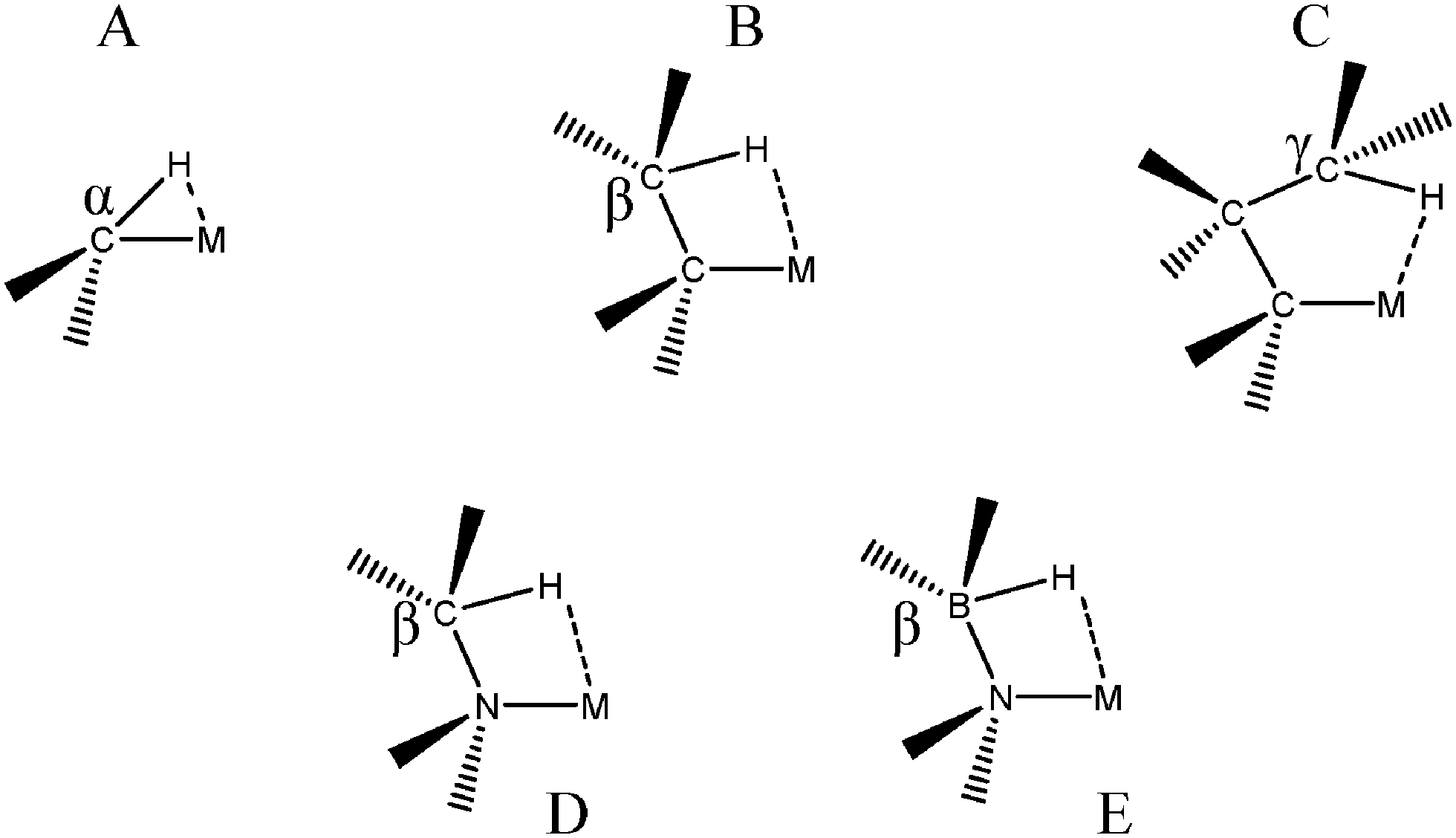 | ||
| Fig. 1 Types of agostic bonds that will be investigated in the present study. | ||
From an experimental point of view, the characterization of an agostic bond is mainly based on four criteria:18
• crystallographic data,
• NMR chemical shifts to high field δ = −5 to −15 ppm,
• reduced NMR coupling constants 1J = 75 to 100 Hz,
• low vibrational frequencies νC–H = 2700–2300 cm−1.
As far as geometric properties are concerned, Brookhart and Green proposed in their seminal article,7 the criteria summarized in Table 1 may be used to distinguish between an agostic and an anagostic interaction:
| M⋯H–C agostic | M⋯H–C anagostic | |
|---|---|---|
| Distance M⋯H (Å) | 1.8–2.3 | 2.3–2.9 |
Angle  (°) (°) |
90–140 | 110–170 |
• Based on QTAIM calculations, five topological criteria were proposed to characterize agostic bonding:18
• a triplet of concomitant topological objects: a bond critical point, a bond path and an interatomic surface,
• a ring critical point, that is a signature of a structural instability,
• a Laplacien of the electron density of the bond critical point ∇2ρBCP in the 0.15–0.25 a.u. range,
• a negative net charge for an hydrogen atom involved in an agostic bonding,
• a dipolar polarization that is 15–30% larger for an agostic hydrogen compared with a non-agostic one.
However, these criteria are not unambiguous since they cannot be applied to any type of agostic bonding, as it will be further discussed in part III.
2. Other definitions
In addition with the rigorous initial definition, the term “agostic” is also sometimes used in a broader definition,21 to characterize intermolecular interactions, especially in the context of sigma alkane,22,23 silane24,25 and sigma boranes.25,26In an attempt to fully characterize some systems potentially containing weak agostic interactions, experimental and theoretical approaches were applied to numerous and various organometallic complexes characterized by geometric distortions. While in some cases clear agostic bonds were identified, in some other systems the approaches used failed to characterize such interactions. The term “anagostic” was proposed to define systems where an interaction between a σ bond and a metallic center leads to a geometric distortion of the structure whereas some considered criteria are not met to label this interaction as “agostic”.27–29
In most of the above-mentioned studies, the agostic interaction occurs in an organometallic complex centered on a metallic atom. In a wider sense however, this concept was employed to qualify situations in which organic molecules interact with metallic surfaces during catalytic processes in the heterogeneous phase. For instance, mechanisms involving agostic interactions were proposed in the chemisorption of hydrogen, hydrocarbons and intermediates on Pt(111).30,31 The formation of a particularly rare agostic interaction was even proposed in the context of the water dissociation of a Pt(111) surface, in combination with hydrogen bonding.32
III. Theoretical characterization of agostic bonding
1. Equilibrium geometry
Since agostic interactions are generally defined on the basis of geometric criteria, geometry optimization may appear as a suitable tool to investigate this type of interactions. Such an approach may complement X-ray structure analyses. In some cases however, the complexes cannot be isolated in the crystalline form (especially in the case of dynamic systems), and a theoretical approach may be the only way to determine whether an agostic interaction is involved in a given reaction pathway. In such a case, particular care should be taken in the choice of the level of theory. In the case of density functional theory calculations, the choice of the functional, the description of the metallic atom as well as the basis set are crucial in the geometrical parameters that will be obtained. Furthermore, in a rigorous theoretical characterization of agostic bonds, such geometry optimizations would only correspond to the first step of a more complete investigation involving either a description in terms of molecular orbitals, or a topological study. As an example, Cho has investigated the agostic structure of titanium methylidene hydride at 15 different levels of theory using Hartree–Fock, Density Functional Theory and Post-Hartree–Fock calculations. He has shown the importance of the choice of the basis set on the agostic distortions, and on the delocalization energies as calculated using the Natural Bond Orbital (NBO) method (vide infra).33 The influence of the basis set superposition error (BSSE) was also underlined by several studies. As an example, the α-agostic interaction involved in Cp*Rh(CO)(η2-alkane) was investigated at various levels of theories,34,35 and the lack of BSSE correction in the conventional ab initio methods leads to an overestimation of the agostic bonding, while some DFT approaches underestimate this interaction.36 Multi-configurationally quantum chemical methods (complete active space self-consistent field (CASSCF)/second-order perturbation theory (CASPT2)) is a powerful approach to compare the agosticity of several metallic centers. Such an approach was used by Roos et al. to explain experimental results in the case of methylidene metal dihydride complexes.372. NBO
Agostic interactions may be seen as donor–acceptor systems, with an electron transfer from a σ bond of the ligand to an unoccupied orbital of the metallic atom. In this respect, techniques for the studies of molecular orbitals may shed some light onto agostic bonding. Natural Bond Orbital theory is a powerful approach to characterize donor and acceptor groups in a molecule, and to quantify delocalization energies. In the natural bond orbital approach, a suite of mathematical algorithms are used to diagonalize the density matrix generated during Hartree–Fock, Density Functional Theory or Post Hartree–Fock calculations. These mathematical transformations allow the generation of orbitals in terms of effective atom-like constituents within the molecular environment.38–40 This approach allows the study of delocalization from atomic orbitals. Toward the natural population analysis, the NBO approach offers a quantitative way to characterize the donor–acceptor relationship. An interesting example of the use of NBO for a quantitative study of agostic bonding is given in the work of Cho et al.33,41 Based on a systematical study, a methodology was proposed to analyze the C–H⋯M agostic bonds in terms of donor–acceptor analysis as defined in the NBO theory.42 Thus, the NBO method provides a valuable way to evaluate the agostic character of interactions.433. QTAIM
In addition to an orbital description of agostic interactions, topological tools were applied in an attempt to qualitatively and quantitatively investigate these bonds. Two topological approaches were particularly applied to the study of agostic bonding: the Bader's quantum theory of atom in molecules (QTAIM) and the electron localization function (ELF). These topological descriptions are based on the dynamical analysis of gradients, from the electronic density, or from functions of electronic density. A vector field is derived from gradients of a potential, and critical points are defined on the basis of the vector fields.The QTAIM approach is based on a partition of the molecular space into non-overlapping regions within which the local virial theorem is fulfilled. This implies, that the kinetic energy of each of these regions has a definite value which is achieved if and only if the integral of the Laplacian of the electron density, ∇2ρ(r), over each region vanishes, a condition which is fulfilled for boundaries which are zero-flux surfaces for the gradient of the density.44 In this method, gradient fields of the electron density ∇ρ(r) are studied. Since an atomic center corresponds to a local maximum of electron density, each atomic center acts as an attractor, and field lines define a basin. Basins are separated from each other by zero-flux surfaces. On each zero-flux surface, gradient lines converge toward a critical point called a bond critical point (BCP). The presence of such a BCP is one of the criterion that was proposed by Popelier et al. to characterize an agostic bond in the QTAIM framework.18,45 On the other hand, the identification of BCP may be difficult in the case of weak agostic interactions. In their systematic study of a set of 20 crystal structures potentially characterized by agostic bonding, Thakur and Desiraju noticed that NBO may be more relevant than QTAIM in describing these weak interactions.33 Numerous studies have now proven that QTAIM can indeed describe β C–H agostic interactions,46,47 but is not suitable for the study of α C–H agostic interactions or weaker interactions such as C–C agostic bonds.48 Indeed, the use of new local criteria seem to be the only way to detect weak agostic bonding by means of the QTAIM approach.49
4. ELF
The ELF approach50–52 intends to provide a partition into basins of attractors which closely match the VSEPR electronic domains, or in other words Lewis's representation. The assumption that groups of electrons can be localized within space filling non-overlapping domains implies that the variances (the squared standard deviation) of the domain populations are minimal. It was pointed out that it is convenient to define a localization function η(r) such as:53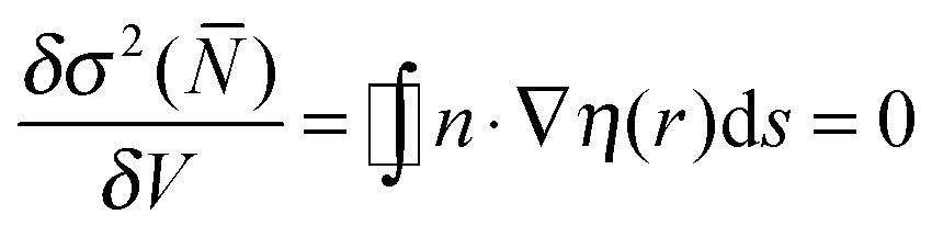 | (1) |
 | (2) |
 | (3) |
 where
where  is the population operator introduced by Diner and Claverie55 and
  is the basin population. The minimization is carried out with the help of the local covariance measure for σ spin electrons:
 | (4) |
The covariance can be written as the sum of four spin components, i.e.:
| σ2(ΩA,ΩB) = σαα2(ΩA,ΩB) + σαβ2(ΩA,ΩB) + σβα2(ΩA,ΩB) + σββ2(ΩA,ΩB) | (5) |
σαα2(ΩA,ΩB) = ![[capital Pi, Greek, macron]](https://www.rsc.org/images/entities/i_char_e136.gif) αα(ΩA,ΩB) − αα(ΩA,ΩB) − ![[N with combining overline]](https://www.rsc.org/images/entities/i_char_004e_0305.gif) α(ΩA)α(ΩB) α(ΩA)α(ΩB) | (6) |
| σαβ2(ΩA,ΩB) = αβ(ΩA,ΩB) − α(ΩA)β(ΩB) | (7) |
| σβα2(ΩA,ΩB) = βα(ΩA,ΩB) − β(ΩA)α(ΩB) | (8) |
| σββ2(ΩA,ΩB) = ββ(ΩA,ΩB) − β(ΩA)β(ΩB) | (9) |
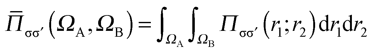 is the number of σσ′ electron pairs between ΩA and ΩB. The opposite spin contributions are expected to be negligible with respect to the same spin ones, and, in fact they are null in the Hartree–Fock approximation. Except for specific delocalized bonding situations such as charge-shift bonds, the covariance between non adjacent basins is negligible. The zero flux surfaces of the gradient field of the spin pair composition for which ELF is an excellent approximation, provide a partition which nearly minimizes the covariance between basins limited a same separatrix.56
The ELF partition yields basins of attractors clearly related to Lewis's model: core and valence basins. A core basin surrounds a nucleus with atomic Z > 2, it is a single basin for the elements of the second period or the union of the basins belonging to the inner shells for heavier elements. It is labelled C(A) where A is the element symbol. In the study of systems involving transition metal elements it is often useful to consider independently the basins of the metal external core (subvalence) shell. The valence basins are characterized by the number of atomic valence shells to which they participate, or in other words by the number of core basins with which they share a boundary. This number is called the synaptic order. Thus, there are monosynaptic, disynaptic, trisynaptic basins, and so on. Monosynaptic basins, labelled V(A), correspond to the lone pairs of the Lewis model, and polysynaptic basins to the shared pairs of the Lewis model. In particular, disynaptic basins, labeled V(A, X), correspond to two-centre bonds, trisynaptic basins, labeled V(A, X, Y), to three-centre bonds, and so on. The valence shell of a molecule is the union of its valence basins. As hydrogen nuclei are located within the valence shell they are counted as a formal core in the synaptic order because hydrogen atoms have a valence shell. For example, the valence basin accounting for a C–H bond is labeled V(C,H) and called protonated disynaptic. The valence shell of an atom, say A, in a molecule is the union of the valence basins whose label lists contain the element symbol A.
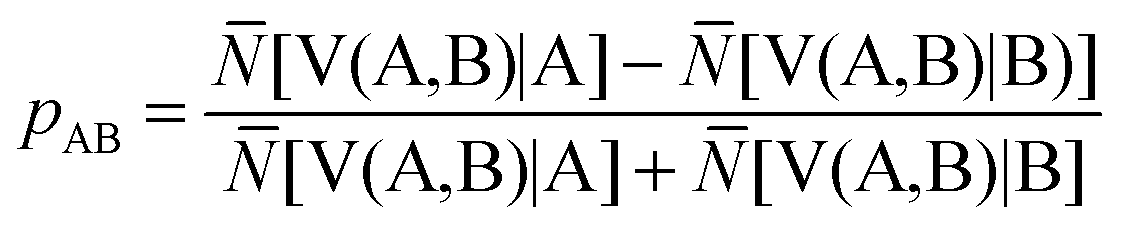
The ELF population analysis provides not only the basin populations and the associated covariance matrix but also the probability of finding n electrons in a given basin and the contribution of the QTAIM basins to the ELF basins. The contribution of the atomic basin of A to the ELF disynaptic basin V(A,B) which is denoted by N[V(A,B)|A] is evaluated by integrating the electron density over the intersection of the V(A,B) basin and of the atomic basin of A. Raub and Jansen57 have introduced a bond polarity index defined as:
 | (10) |
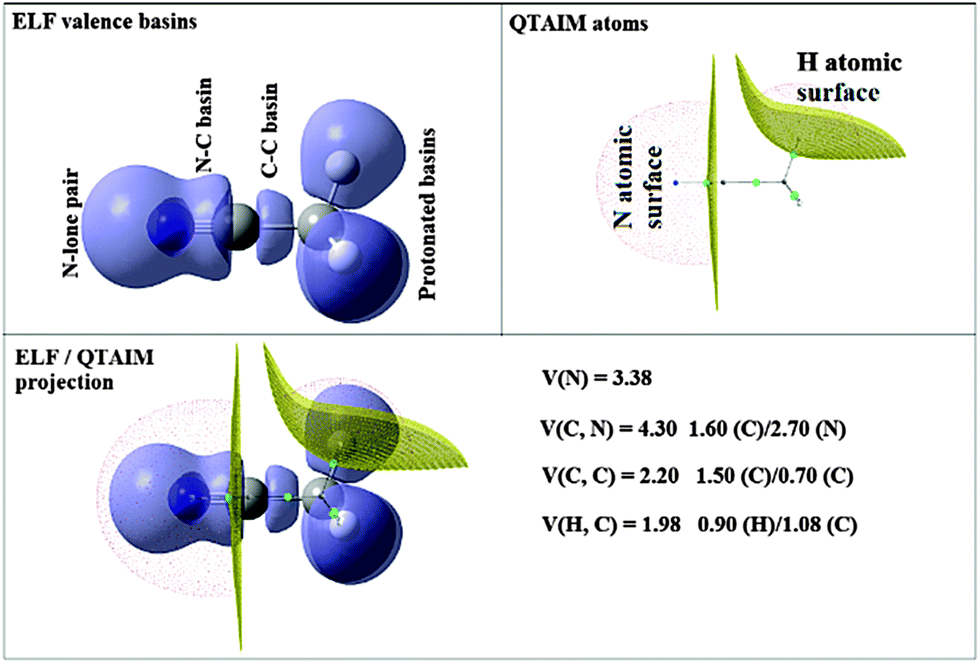 | ||
| Fig. 2 QTAIM and ELF basins for the free NCCH3 molecule. | ||
IV. Topological descriptions, probabilistic approach and qualitative estimators
1. Context
ELF has proven to be a valuable tool for characterizing all kinds of chemical bonds. In the case of weak interactions such as 2c–3e and hydrogen bonding, the ELF analysis enables us to describe and classify them in terms of topological properties very close and similar to the traditional chemical concepts.The analysis of basin population was helpful to distinguish between weak, medium and strong hydrogen bonding. It was shown that the core–valence bifurcation index is a suitable criterion to quantitatively describe these interactions.17,58
In the case of 2c–3e bonding, no disynaptic basins are found. However, this is not the sole criterion to determine whether a bonding exists or not, and once again, core–valence bifurcation index has proved to be a very powerful tool. In addition, in this specific case, a topological delocalization index was helpful in quantifying the electron fluctuation.59,60
These examples prove that, beyond the BCP, topological approaches can be used in a quantitative way to thoroughly characterize electron localization/delocalization involved in different types of interactions. Below we will present a similar approach to characterize agostic interactions.
2. Presentation of the approach
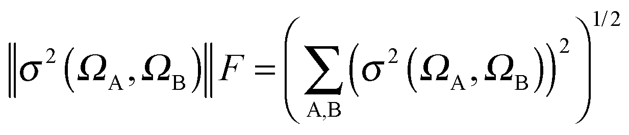
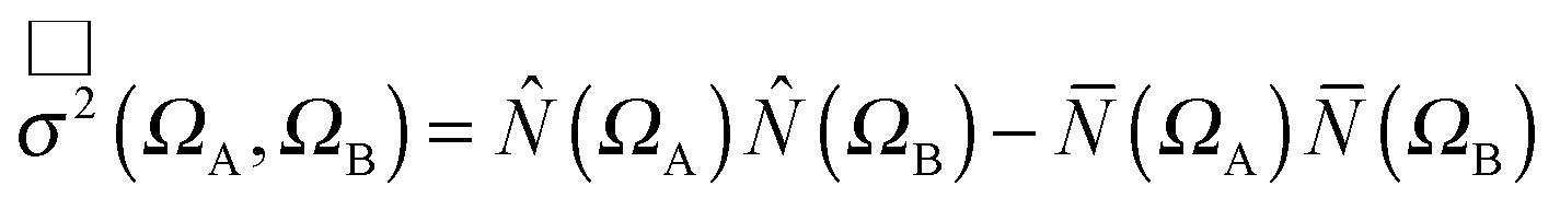
The multivariate analysis is a basic statistical method enabling one to reveal the correlations between different groups of data. It relies upon the construction of the covariance matrix elements defined by
| 〈cov(i,j)〉 = 〈ij〉 − 〈i〉〈j〉 | (11) |
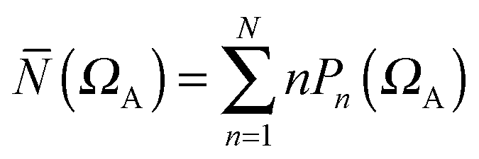
The bonding in most molecular systems can be described by a strict localization of electron pairs. A more realistic picture, closely related to the concept of resonance, is provided by the superposition of electron multiplets distributed among the basins and therefore accounting for the electron delocalization. The population of a given basin ΩA appears accordingly as the average of such n-tuplets weighted by the probability, Pn(ΩA) of finding n electron in ΩA:
 | (12) |
In our search for several parameters to qualitatively estimate the strength of agostic bonding, we studied a large number of systems. From this study, it was found that four parameters from QTAIM and ELF taken together may allow a comparison of agostic bonding present in different systems between the X–H bond (X = C, B…) and a metallic center M:
• First of all, we will consider only hydrogen atoms as potentially involved in agostic interactions. In the Brookhart and Green's definition,6,7 even if this is not the only criterion, the presence of three atomic centers sharing two electrons is the fundamental aspect of agostic bonding. Thus, in the topologic description, the total population of the protonated potentially agostic basin V(H) is an obvious important parameter.
• The projection of ELF on AIM basins gives some information on the atomic contribution in the agostic protonated basin. Hereafter in this paper, this quantity will be labeled as M/X/H in the case of the X–H agostic bond (X = C or B). Hereafter, this information will be used as a clear indicator of the trisynaptic character of a protonated basin. It is worthy to note that an atomic contribution only makes sense if its value is larger than the numerical error, i.e. 0.01 electron.
• The covariance calculated from the ratio between the basin's population of the potentially agostic H atom and the population of the metallic center core basin C(M) is an important parameter to characterize the interaction between these two basins Cov(V(H)/C(M)). The covariance thus obtained from ELF topological analysis gives some insights into the delocalization of electrons between the two atoms. Obviously this value depends on the theoretical description of the metallic center: the covariance is smaller when a pseudo potential is used for the metallic center. Taken together with the previous parameters, a covariance larger than 0.03 (in absolute value) is a proof of an agostic interaction between the X–H σ bond and M.
• Furthermore, in the context of comparison between several levels of calculations, the σ2 and the variance calculated with the ELF topological approach are an indication of deviation from perfect localization coming from inter-population. Similar values of variances for a same system calculated at different levels of theories thus allows us to ensure that all the theoretical descriptions are consistent with each other.
Furthermore, it was shown that the electron density (ρ) of the bond critical point (BCP) could be related to the bond order and thus the bond strength.62 We propose the use of three ρ(BCP) to gain some insight into the strength of the agostic interaction. In line with Popelier and Logothetis,18 we suggest the use of the ρ(BCP) of the M–Hβ bonding, when it exists. Additionally, the comparison of the ρ(BCP) values associated with the C–Hagostic and C–Hfree allows us to estimate the weakening of the C–Hagostic bond caused by the agostic interaction. Two conditions are necessary for the use of the ρ(BCP(C–Hagostic)) and ρ(BCP(C–Hfree)) values. First, the carbon bearing the hydrogen atom potentially involved in an agostic interaction should also bear an additional non-agostic hydrogen atom. This condition is often fulfilled. Furthermore, neither of the Hagostic and Hfree atoms should be involved in another non-covalent interaction. Provided that these conditions are satisfied, we can propose the following reference values. In the alkyl complexes, the ρ(BCP(C–Hfree)) are characterized by
| 0.28 ≤ ρ(BCP(C–Hfree)) ≤ 0.29 |
| 0.200 ≤ ρ(BCP(C–Hagostic)) ≤ 0.27 |
From the ELF point of view, a protonated basin is considered as a trisynaptic basin when its population originates from three atomic centers. An H-agostic bond is a protonated trisynaptic basin whose population is around 2e−. Consequently, it corresponds to the traditional 3c–2e interaction in chemistry.
These parameters were not only chosen for their ability to describe an agostic interaction, but also for their phenomenological significances. Indeed, the increase in covariance Cov(V(H)/C(M)) signifies that the delocalization of electrons between the metallic center and the agostic protonated basin increases, concomitantly with a weakening of the bond between the hydrogen and other atom X. The H–X bond is thus activated and the agostic character of the interaction between H and M is stronger. In a limit case, when the agostic bonding becomes stronger and stronger, the ELF basin evolves from a trisynaptic to a disynaptic basin, and the covariance increases till the formation of a covalent M–H bond. This corresponds to a metallic hydride.
Moreover, the strength of an agostic H–X bond may be estimated from the QTAIM properties calculated at the H–X bond critical point (BCP). Interestingly, the charge density at the agostic H–X BCP compared to that of a non-agostic H–X bond in the complex (and/or compared to the charge density at the H–X BCP of free ligand) provides an indication to the strength of the agostic interaction.
From this study as well as from further theoretical investigations, it was found that QTAIM suitably describe β C–H and γ C–H agostic bonds, but not the α C–H ones, even in cases for which experimental data tend to prove that α C–H agostic bonds were indeed formed.
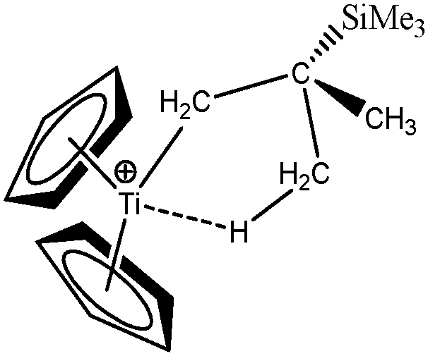
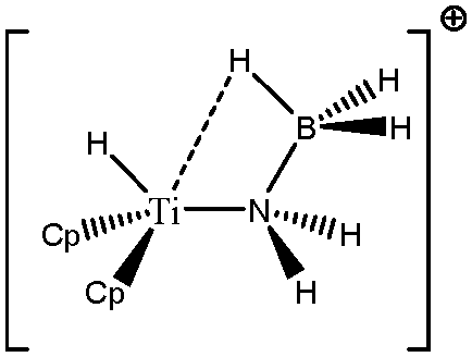
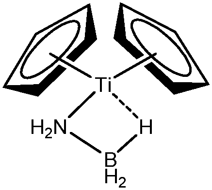
Some compounds were observed under different agostomers. We will choose a few examples of agostomers based on experimental investigations carried out by Baird et al.63,64 In the case of [Cp2TiCH2CHMe t-Bu]+, they observed that the α-agostic isomer is preferentially formed although a β-agostic isomer could have been formed. Such a situation is relatively rare: when both α-and β-agostic isomers may be formed, generally the β-agostic form is more stable. Another alkyl–titanium complex that may exist as β- and γ-agostomers will be considered.
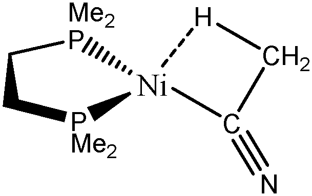
The complex formed between acetonitrile and zero-valent nickel that may lead to the formation of a C–H agostic bond65 will be investigated.
In an attempt to understand the parameters that influence the formation of agostic bonds, the effect of co-ligands, small changes in the structures and the nature of the metallic center, will be investigated. The effect of the presence of a co-ligand will be topologically investigated based on the example of a rhodium thiophosphoryl pincer complex studied by Milstein et al.66
Different titanium complexes will be compared, based on the compounds studied by Popelier,18 Baird63,64 and Mc Grady.67 The comparison of complexes studied by Mc Grady67 and Forster68 will allow the study of influence of the nature of the metallic center. Further examples derived from the model compounds of Popelier18 as well as from Sabo-Etienne69 will also be discussed.
Lastly, interactions involving heteroatoms will be considered. Indeed, such interactions are sometimes considered as “agostic” whereas some authors consider that all the contribution from a σ bond and an unoccupied orbital of a hypovalent transition metal center cannot be classified under an unique appellation. Our aim here is to determine whether the methodology above presented is able to differentiate between these types of interactions, or whether these interactions are due to a similar effect. For this purpose, titanocene and zirconocene amidoborane complexes,67,68 dimethylaminoborane complexes,69 and mesitylborane complexes70 will be considered. The last examples correspond to intermolecular interactions, whereas in the other systems, the weak interaction between a σ X–H bond and the metal center should be considered as an intramolecular interaction.
V. Application to a representative set of examples
1. Influence of the level of theory
To begin with, the influence of the level of theory on the parameters calculated with the ELF topology will be checked. To this end, DFT calculations were carried out, and three different types of functionals were selected:• B3LYP because this is one of the most popular hybrid functional,
• PBE0 because this is a non-empirical hybrid functional71 that was widely employed in the context of agostic interactions,
• TPSSh because this meta-GGA hybrid functional can be used for reference calculations, when combined with a suitable basis set.72
In combination with these functionals, six different basis sets were selected:
• the 6-311++G(2d,2p) basis set, in combination with a pseudo-potential LANL-2TZ-f including a triple ξ and an additional diffuse f function for the metallic center,
• the 6-311++G(2d,2p) basis set, in combination with a pseudo-potential LANL-2TZ-p including a triple ξ and an additional diffuse p function for the metallic center,
• the 6-311++G(2d,2p) basis set, in combination with a pseudo-potential LANL-2DZ including a double ξ function for the metallic center,
• the 6-31++G(2d,2p) basis set, in combination with a pseudo-potential LANL-2DZ including a double ξ function for the metallic center,
• the 6-311++G(2d,2p) basis set, without any pseudo potential for the metallic center,
• the 6-31++G(3df,3pd) basis set, without any pseudo potential for the metallic center.
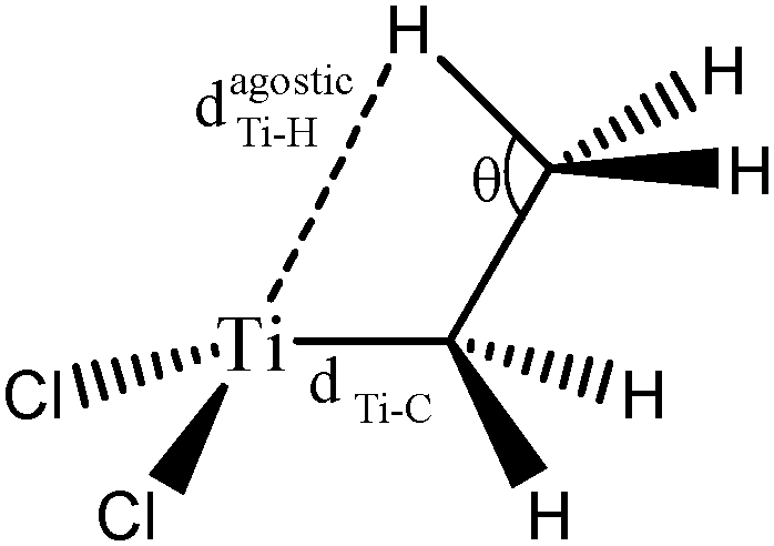
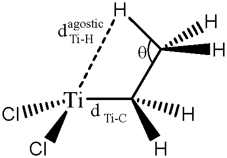
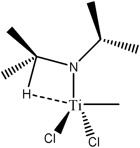
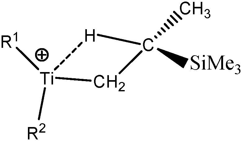
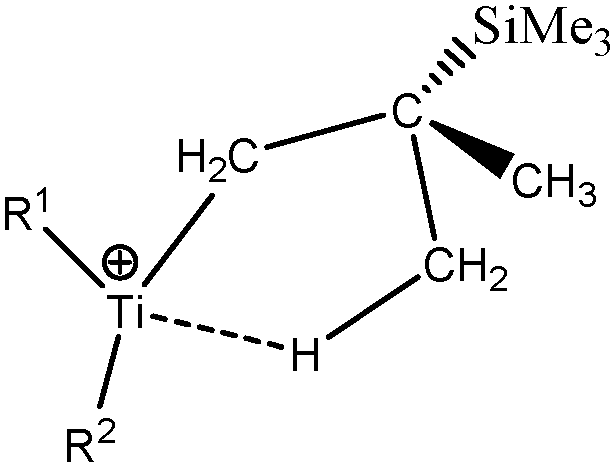
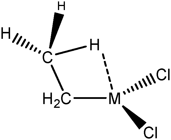
For these tests of the influence of the levels of theories, a simple model molecule taken from the study of Popelier and Logothetis was selected (see below, [TiCl2CH2CH3]+).
In a first series of tests, the molecule was re-optimized at each level of theory prior to the topological investigation. In a second series of tests, the complex was optimized using the highest level of theory, namely B3LYP, PBE0, or TPSSh/6-31++g(3df,3pd), and ELF calculations were then carried out on the wave function of the single point geometries using the LanL2DZ as the basis set.
Optimized geometries are compared in Table 2 and the topological parameters are summed up in Table 3.
| Level of theory | d(Ti–C) (Å) | d(Ti–Hagostic) (Å) | θ (°) | |
|---|---|---|---|---|
|
B3LYP/6-311++G(2d,2p) | 2.008 | 2.034 | 113.8 |
| B3LYP/6-311++G(3df,3pd) | 2.008 | 2.030 | 113.8 | |
| PBE0/6-311++G(3df,3pd) | 1.986 | 2.015 | 114.3 | |
| TPSSh/6-311++G(3df,3pd) | 2.009 | 2.008 | 113.5 |
| Level of theory | V(Hβ) | Ti/Cβ/Hβ | Cov(V(Hβ)/C(Ti)) | σ 2 | d(Ti–Hagostic), θ, d(Ti–C) | |
|---|---|---|---|---|---|---|
| B3LYP | Lanl2DZ | 1.89 | 0.04/0.82/1.03 | −0.08 | 0.72 | 2.116, 115.6, 1.982 |
| 6-31++G(2d,2p) | 1.95 | 0.08/0.78/1.09 | −0.09 | 0.74 | 2.034, 113.8, 2.003 | |
| 6-311++G(2d,2p) | 1.93 | 0.08/0.76/1.09 | −0.09 | 0.73 | 2.034, 113.8, 2.008 | |
| 6-31++G(2d,2p)/LanL2DZ | 1.92 | 0.03/0.78/1.11 | −0.09 | 0.72 | 2.025, 113.7, 1.994 | |
| 6-311++G(2d,2p)/LanL2DZ | 1.92 | 0.04/0.75/1.13 | −0.09 | 0.73 | 2.005, 113.4, 1.996 | |
| 6-311++G(2d,2p)/LanL2TZ(P) | 1.90 | 0.04/0.73/1.13 | −0.10 | 0.72 | 2.009, 113.6, 2.004 | |
| 6-311++G(2d,2p)/LanL2TZ(F) | 1.90 | 0.05/0.72/1.13 | −0.10 | 0.72 | 2.005, 113.4, 2.002 | |
| PBE0 | 6-31++G(2d,2p) | 1.93 | 0.07/0.78/1.08 | −0.09 | 0.74 | 2.019, 114.4, 1.983 |
| 6-311++G(2d,2p) | 1.92 | 0.07/0.77/1.08 | −0.10 | 0.74 | 2.018, 114.3, 1.986 | |
| 6-31++G(2d,2p)/LanL2DZ | 1.91 | 0.04/0.75/1.12 | −0.10 | 0.73 | 2.002, 117.0, 1.975 | |
| 6-311++G(2d,2p)/LanL2DZ | 1.91 | 0.04/0.75/1.12 | −0.10 | 0.73 | 1.985, 113.9, 1.977 | |
| 6-311++G(2d,2p)/LanL2TZ(P) | 1.90 | 0.04/0.74/1.12 | −0.10 | 0.74 | 1.990, 114.1, 1.985 | |
| 6-311++G(2d,2p)/LanL2TZ(F) | 1.90 | 0.05/0.73/1.12 | −0.10 | 0.73 | 1.989, 114.1, 1.982 | |
| TPSSH | 6-31++G(2d,2p) | 1.93 | 0.08/0.74/1.11 | −0.10 | 0.73 | 2.016, 113.6, 2.006 |
| 6-311++G(2d,2p) | 1.93 | 0.08/0.74/1.11 | −0.10 | 0.72 | 2.011, 113.5, 2.009 | |
| 6-31++G(2d,2p)/LanL2DZ | 1.93 | 0.03/0.77/1.13 | −0.10 | 0.73 | 2.001, 113.4, 1.995 | |
| 6-311++G(2d,2p)/LanL2DZ | 1.90 | 0.03/0.72/1.15 | −0.09 | 0.72 | 1.980, 113.1, 1.996 | |
| 6-311++G(2d,2p)/LanL2TZ(P) | 1.91 | 0.04/0.72/1.15 | −0.10 | 0.73 | 1.985, 113.3, 2.005 | |
| 6-311++G(2d,2p)/LanL2tz(F) | 1.91 | 0.04/0.72/1.15 | −0.10 | 0.72 | 1.985, 113.3, 2.002 | |
| SP | B3LYP/LanL2DZ//B3LYP/6-311++G(3df,3pd) | 1.83 | 0.03/0.73/1.07 | −0.08 | 0.72 | Single-point calculations |
| PBE0/LanL2DZ//PBE0/6-311++G(3df,3pd) | 1.89 | 0.03/0.82/1.04 | −0.08 | 0.73 | ||
| TPSSh/LanL2DZ// | 1.89 | 0.02/0.81/1.06 | −0.08 | 0.72 | ||
| TPSSh/6-311++G(3df,3pd) | ||||||
The values presented in Table 2 clearly show that the geometry of the complex is correctly described even with the B3LYP functional, when used in combination with a relatively large basis set including 2d and 2p polarization functions. Indeed, if we compare the distances and the angles calculated at the B3LYP/6-311++G(2d,2p) level of theory with the reference values (calculations at the TPSSh/6-311++G(3df,3pd) level of theory), the errors are 0.001 Å, 0.026 Å and 0.3° for the d(Ti–C), d(Ti–Hagostic), and θ, respectively.
Table 3 clearly shows that all the selected levels of theory identify an agostic bonding in this simple TiCl2–alkyl system. Indeed,
• the total population of the valence basin of Hβ is slightly smaller than 2e−,
• the variance value (σ2) does not depend on the level of theory which indicates the stability of the ELF topological procedure in partitioning the molecular space,
• in all the cases, the contribution of the titanium atom to this basin is in the range of 0.07–0.08 e− provided to use an explicit triple zeta quality basis set for metallic center,
• the calculated covariance is close to −0.1, clearly indicating a delocalization of the electrons between agostic hydrogen and a metallic center.
These four criteria should be considered all together, the presence or the absence of one of the criterion is not sufficient to drive any conclusion.
We would like to emphasize the fact that, whatever the level of theory selected, the topological analysis of the agostic bonding leads to similar results. Thus, the criteria selected are robust toward the level of theory.
This study thus show that the B3LYP/6-311++G(2d,2p) can be used for a topological investigation of agostic interactions. This level of theory was selected for all the further studies presented below.
2. Study of different agostomers
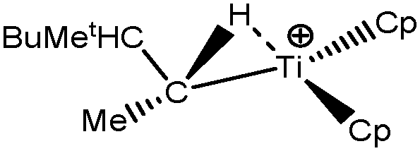
Let us first consider alkyl titanocene compounds [Cp2TiCH2CHMe(t-Bu)]+ studied by Baird et al.63 Two agostic isomers were characterized: α- and β-agostomers (Fig. 3).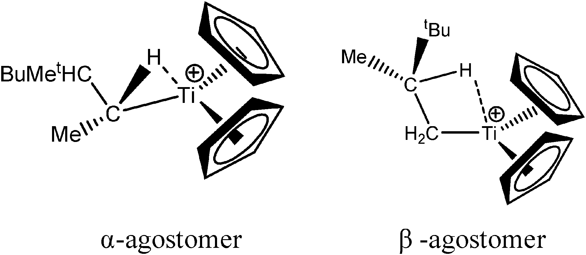 | ||
| Fig. 3 α- and β-agostomers observed for an alkyl titanocene compound.63 | ||
The experimental study clearly shows that, between two diastereoisomers α- and β-agostic, the α-agostic one is more stable. The Table 4 shows, without any surprise, that a BCP is indeed obtained in the case of the β-agostic isomer that is not the case for the α-agostic one. Nevertheless, it is worth noting that the electron density at the C–H bond slightly decreases by 0.05 a.u. due to the agostic deformation for both α- and β-agostic isomers. Simultaneously, the Laplacian of charge density (∇2ρ) and the energy density (H) at the BCP increase, leading to the reduction of the covalent character of the C–H bond.
| α-agostomer | β-agostomer |
|---|---|
| BCP(Ti–Hα): does not exist | BCP(Ti–Hβ): ρ = 0.03, ∇2ρ = +0.11, H = 0.00, ε = 0.37 |
| BCP(Ti–Cα): ρ = 0.10, ∇2ρ = +0.07, H = −0.04 | RCP(Ti–Hβ–Cβ): ρ = 0.03, ∇2ρ = +0.13 |
| BCP(Cα–Hα): ρ = 0.24, ∇2ρ = −0.70, H = −0.23 | BCP(Ti–Cα): ρ = 0.10, ∇2ρ = +0.03, H = −0.04 |
| BCP(Cα–H): ρ = 0.29, ∇2ρ = −1.05, H = −0.31 | BCP(Cα–H): ρ = 0.29, ∇2ρ = −1.04, H = −0.31 |
| BCP(Cα–Cβ): ρ = 0.24, ∇2ρ = −0.51, H = −0.19 | BCP(Cα–Cβ): ρ = 0.24, ∇2ρ = −0.49, H = −0.19 |
| BCP(Cβ–H): ρ = 0.29, ∇2ρ = −1.03, H = −0.30 | BCP(Cβ–Hβ): ρ = 0.24, ∇2ρ = −0.69, H = −0.22 |
To further characterize these two isomers, the methodological approach above proposed was applied, and Table 5 summarizes the ELF investigation of these two isomers.
| Isomer |
|
|
|---|---|---|
| Ti-alpha-Baird | Ti-beta-Baird | |
| V(H) | 1.89 | 1.9 |
| M/X/H | 0.04/0.78/1.07 | 0.04/0.80/1.11 |
| Cov(V(H)/C(M)) | −0.09 | −0.06 |
| d(Ti–Hagostic) (Å) | 2.05 | 2.01 |
| d(C–Hagostic) (Å) | 1.14 | 1.17 |

The results presented in Table 5 clearly show that, despite the absence of BCP in the alpha agostomer, the agostic bonding is indeed described by the combined ELF/QTAIM studies. Indeed, the total population of the valence basin of Hα is below 2e−, the contribution of the Ti atom to the protonated valence basin of Hα is 0.04, which is not negligible, and the covariance between two basins VHα/CM is close to −0.1. In comparison, the total population of the agostic H atom is closer to 2e− and the covariance is slightly smaller (in absolute value) in the case of the β-agostic isomer. As a conclusion, the agostic character is slightly more pronounced in the α-agostic isomer compared with the β-agostic one, for this specific case. Furthermore, these two agostic bonds are relatively weak.
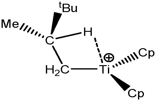
Baird et al.64 also studied an alkyl–titanium complex that exist under two isomeric forms, one presenting a β-agostic bonding, and another presenting a γ-agostic bonding. Table 6 summarizes the ELF/QTAIM characteristics of these two isomers. As in the previous case, the statistical parameters of ELF clearly describe both agostic bonds. These bonds are characterized by BCP's and RCP's in the QTAIM description. The quantitative study of these bonds shows that the σ C–H interactions are relatively weak, as it was the case in the previous α- and β-agostic isomers.
| Isomer |
|
|
|---|---|---|
| Ti-beta-Si-Baird | Ti-gamma-Si-Baird | |
| V(H) | 1.93 | 1.95 |
| M/X/H | 0.06/0.77/1.10 | 0.05/0.81/1.09 |
| Cov(V(H)/C(M)) | −0.08 | −0.07 |
| d(Ti–Hagostic) (Å) | 2.09 | 2.00 |
| d(C–Hagostic) (Å) | 1.16 | 1.15 |
As a conclusion, these examples show that the topological tools of the ELF approach indeed allows the characterization of α-, β- and γ-agostic bonds.
3. Topological characterization of a representative set of C–H agostic bonds
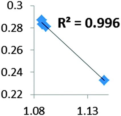
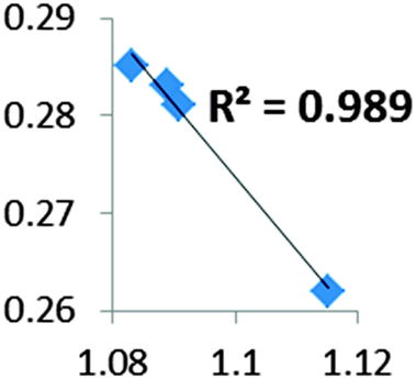
A set of complexes was used to probe the agostic character of different features of M⋯H–C bonding by means of the topological criteria previously presented, and the selected topological criteria are summarized in Table 7.| Compound |
|
|
|
|
|---|---|---|---|---|
| Ti-Popelier18 | Ti-alpha-Baird63 | Ti-beta-Baird63 | EtTiCl3(dmpe)-McGrady67 | |
| V(H) | 1.93 | 1.90 | 1.96 | 1.97 |
| M/X/H | 0.08/0.76/1.09 | 0.04/0.79/1.07 | 0.04/0.81/1.11 | 0.03/0.94/1.00 |
| Cov(V(H)/C(M)) | −0.09 | −0.09 | −0.06 | −0.04 |
| d(Ti–Hagostic) (Å) | 2.034 | 2.049 | 2.157 | 2.183 |
| d(C–Hagostic) (Å) | 1.146 | 1.140 | 1.151 | 1.115 |
| ω(C–Hagostic) (cm−1) | 2534 | 2589 | 2429 | 2815 |
| d(Cα–Hfree) (Å) | 1.0874, 1.0874 | 1.085 | 1.083 | 1.083 |
| ω(C–Hfree) (cm−1) | 3087–3172 | 3037–3134 | 3034–3197 | 3067–3177 |
| QTAIM topological parameters for agostic compound: ρ, ∇2ρ, H(ρ) in a.u. | ||||
| BCP(C–Hβ) | 0.233, −0.67, −0.22 | 0.238, −0.70, −0.30 | 0.235, −0.69, −0.22 | 0.262, −0.86, −0.26 |
| BCP(C–Hfree) | 0.287, −1.07, −0.30 | 0.288, −1.05, −0.31 | 0.288, −1.05, −0.31 | 0.285, −1.03, −0.31 |
| BCP(Ti–Hβ) | 0.045, +0.14, 0.00 | Does not exist | 0.029, +0.11, 0.00 | Does not exist |
| Some relevant parameters for free ligand: | ||||
| d(C–H) (Å) | 1.091 | 1.096 | 1.0908 | |
| ω(C–H) (cm−1) | 3034–03![[thin space (1/6-em)]](https://www.rsc.org/images/entities/char_2009.gif) 101 101 |
2991–3110 | 3034–3101 | |
| BCP(C–Hβ) | 0.281, −1.01, −0.30 | 0.282, −1.01, −0.30 | 0.281, −1.01, −0.30 | |
| Electron density at BCP(C–H) in function of d(C—H) |
|
|
|
|

| Compound |
|
|
|
|
|---|---|---|---|---|
| CpTiNiPr2Cl2-McGrady67 | Rh-butene-Milstein66 | Rh-H2CO-Milstein66 | Ni-Jones65 | |
| V(H) | 2.06 | 2.01 | 2.12 | 2.01 |
| M/X/H | 0.01/1.07/0.98 | 0.05/1.02/0.95 | 0.23/0.93/0.96 | 0.07/0.98/0.96 |
| Cov(V(H)/C(M)) | −0.02 | −0.15 | −0.38 | −0.13 |
| d(Ti–Hagostic) | 2.363 | 1.939 | 1.665 | 1.811 |
| d(C–Hagostic) | 1.095 | 1.131 | 1.222 | 1.126 |
| ω(C–Hagostic) | 3006 | 2612 | 1950 | 2665 |
| d(Cα–Hfree) | 1.088, 1.090, 1.090 | 1.088 | 1.088 | 1.088 |
| ω(C–Hfree) | 3040–3130 | 3174–3192 | 3174–3182 | 3070–3119 |
| QTAIM topological parameters for agostic compound: ρ, ∇2ρ, H(ρ) in a.u. | ||||
| BCP(C–Hagostic) | 0.287, −1.05, −0.30 | 0.250, −0.77, −0.24 | 0.202, −0.47, −0.16 | 0.256, −0.82, −0.25 |
| BCP(C–Hfree) | 0.284, −1.03, −0.30 | 0.281, −0.97, −0.28 | 0.282, −0.98, −0.85 | 0.285, −1.04, −0.30 |
| BCP(M–Hagostic) | Does not exist | 0.055, +0.20, −0.01 | 0.107, +0.26, −0.05 | 0.057, +0.23, −0.01 |
| Some relevant parameters for free ligand: | ||||
| d(C–H) | 1.093 | 1.092 | 1.089 | |
| ω(C–H) | 3020–3040 | 3050 | 3060–3128 | |
| BCP(C–Hβ) | 0.288, −1.06, −0.31 | 0.277, −0.94, −0.28 | 0.283, −1.03, −0.30 | |
| Electron density at BCP(C–H) in function of d(C–H) | Borderline case: if there was an agostic case, it should correspond to a very weak interaction! |
|
|
|
For all the species the total population of the valence basin of the agostic hydrogen atom is in the 2 ± 0.15 e− range. Both the covariance Cov(V(H)/C(M)) and the atomic contributions in the valence basin of H(M,X,H) fluctuate depending on the complex.
Table 7 presents complexes containing intramolecular σ C–H agostic bonding. However, the Rh-H2CO-Milstein66 and Rh-butene-Milstein66 complexes could not be easily classified as β agostic species. We note in passing with these two examples that a change in the nature of a co-ligand may strongly affect the agostic character of a C–H bond. Indeed a weak agostic character is topologically predicted in the case of the Rh-butene-Milstein66 complex, whereas a strong one is predicted for the analogous compound containing H2CO instead of butene as the co-ligand. These two cases will be further discussed hereafter.
A close look of the data reported in Table 7 shows some trends which be summarized as follows:
• In the view of the metal contribution in the protonated basin, we can classify the complexes into four categories: (1) M = 0.01 e corresponding to an undefined case, (2) 0.01 < M < 0.05 for weak–medium agostic bonding, (3) 0.05 < M < 0.20 for medium–strong agostic interaction, and (4) M > 0.20 for almost pre-dissociated C–Hagostic or pre-hydride Hagostic–M.
• One can note that the calculated harmonic vibrational frequency of the C–Hagostic oscillator is always red-shifted with respect to that of C–Hfree. To a certain extent, the amount of this red-shift reflects the strength of the agostic interaction. It is interesting to note that the harmonic vibrational frequency of C–Hfree is sometimes blue-shifted with respect to the C–H frequency in the free ligand. However, on the ground of C–H vibrational frequency red-shift one can easily distinguish three categories of agostic species: red-shift ≈2% for the weakest agostic compound (CpTiNiPr2Cl2-McGrady), red-shift ≈40% for the strongest agostic compound (Rh-H2CO-Milstein), and 5% < red-shift <40% for the other compounds going from weak to strong cases.
• The case of the CpTiNiPr2Cl2-McGrady compound: this compound has been previously considered as an agostic case by McGrady et al.67 and also by Scherer and coworkers.73 We would like to emphasize that the very low metal contribution (0.01 e) in the population of V(H) makes actually impossible to decide the presence or absence of an agostic interaction, because of the numerical uncertainty of our ELF analysis which is just equal to 0.01 e.
This is also consistent with the geometrical properties of the complex: if we refer to the criteria summarized in Table 1, the CpTiNiPr2Cl2-McGrady compound is anagostic (d(M–H) > 2.3 Å).
In order to check the possible effect of the dispersion contribution in the electronic structure, we also optimized the studied structure using two hybrid functionals (wB97XD and B2PLYPD3) which are suitable to treat the very weak non-covalent interactions.
As shown by the results reported in Table 8, topological differences between the Cβ–Hβ so-called agostic bond and Cβ–Hfree within the same compound are minor so that we can confidently exclude a dominant agostic interaction within this complex. This description is also supported by a very small vibrational ω(C–H) frequency shift (less than 2%) with respect to free ω(C–H). Furthermore, we found a BCP between the so-called agostic H atom and one of the two chlorine atoms. At this latter BCP, the electron density is equal to 0.015 e belonging to the hydrogen bonded range.74
| wB97XD | B2PLYPD3 | B3LYP | |
|---|---|---|---|
| d(Cβ–Hβ) (Å) | 1.096 | 1.095 | 1.095 |
| ω(C–H) (cm−1) | 3035 | 3006 | |
| BCP(Cβ–Hβ): ρ, ∇2ρ in a.u. | 0.286, −1.04 | 0.287, −1.05 | 0.284, −1.03 |
| d(Cβ–Hfree) (Å) | 1.091 | 1.090 | 1.090 |
| ω(C–H) (cm−1) | 3077 | 3040 | |
| BCP(Cβ–Hfree): ρ, ∇2ρ in a.u. | 0.290, −1.067 | 0.291, −1.08 | 0.287, −1.05 |
• Agostic bonding and QTAIM bond critical point: we note that the presence of a BCP(H–Ti) in the case of the EtTiCl3(dmpe)-McGrady compound actually depend on the level of theory. Indeed, we found a BCP only at the BP86/6-311++G(d,p) level, whereas there is no BCP(H–Ti) when we use B3LYP, PBE0 or BP86 with 6-311++G(2d,2p) as the basis set.
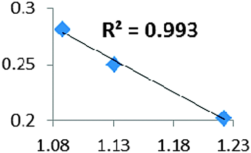
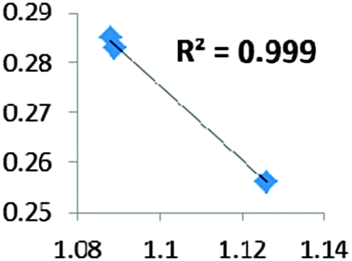
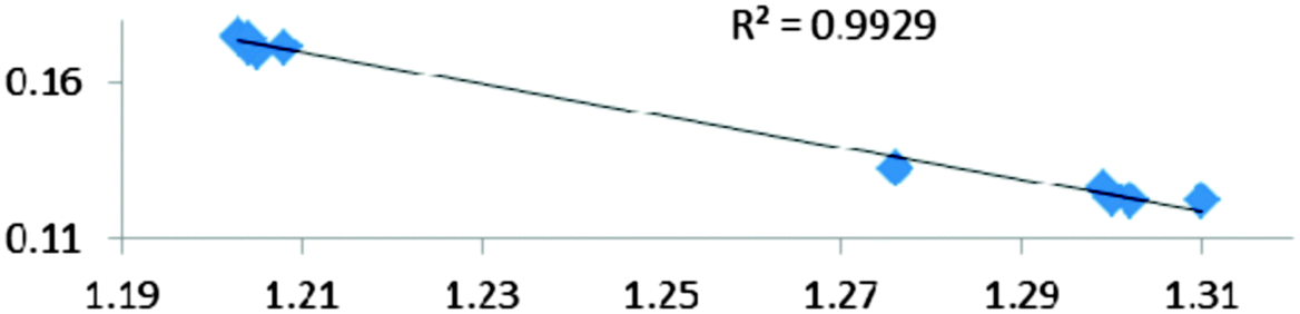
• Concerning the strength of an agostic bond, we note that the electron density at the BCP(C–H agostic) decreases when the agosticity increases. This trend is graphically shown for each compound in Table 7. A global linear regression graph for all the species will be discussed in Section VI.
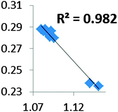
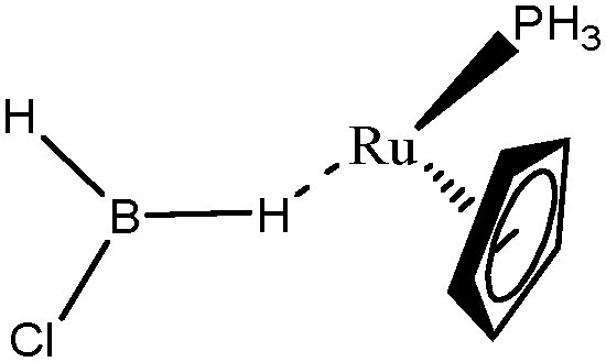
4. Topological characterization of a representative set of B–H agostic bonds
In Table 9 are gathered five complexes containing intramolecular σ B–H agostic bonds. These complexes have been a subject of experimental and/or theoretical study.65,67,68| Compound |
|
|
|
|
|
|---|---|---|---|---|---|
| ZrClNH2BH3-a-Forster68 | ZrClNH2BH3-b-Forster68 | TiHNH2BH3-a-McGrady67 | TiHNH2BH3-b-McGrady67 | TiCp2NH2BH3-McGrady67 | |
| V(H) | 1.89 | 1.92 | 1.89 | 1.85 | 1.92 |
| M/X/H | 0.07/0.22/1.59 | 0.07/0.27/1.58 | 0.07/0.24/1.58 | 0.07/0.26/1.52 | 0.12/0.23/1.57 |
| Cov(V(H)/C(M)) | −0.13 | −0.13 | −0.14 | −0.14 | −0.15 |
| d(M–Hagostic) | 2.030 | 2.039 | 1.892 | 1.855 | 1.892 |
| d(B–Hagostic) | 1.302 | 1.276 | 1.300 | 1.310 | 1.299 |
| ω(B–Hagostic) | 1932 | 2084 | 1959 | 1814 | 1895 |
| d(B–Hfree) | 1.203 | 1.203 | 1.205 | 1.204 | 1.204 |
| ω(B–Hfree) | 2488–2542 | 2487–2539 | 2474–2526 | 2480–2530 | 2477–2524 |
| QTAIM topological parameters for agostic compound: ρ, ∇2ρ, H(ρ) in a.u. | |||||
| BCP(B–Hagostic) | 0.122, +0.02, −0.11 | 0.132, 0.00, −0.13 | 0.123, +0.02, −0.11 | 0.122, −0.01, −0.11 | 0.126, −0.01, −0.12 |
| BCP(B–Hfree) | 0.175, −0.27, −0.20 | 0.174, −0.26, −0.19 | 0.170, −0.21, −0.18 | 0.171, −0.21, −0.18 | 0.174, −0.26, −0.19 |
| BCP(M–Hagostic) | 0.057, +0.11, −0.01 | 0.056, +0.11, −0.01 | 0.059, +0.11, −0.01 | 0.062, +0.13, −0.01 | 0.057, +0.16, −0.01 |
| Some relevant parameters for free ligand: | |||||
| d(B–H) (Å) | 1.208 | ||||
| BCP(B–Hβ) | 0.171, −0.24, −0.19 | ||||
| Electron density at BCP(B–H) in function of d(B–H) |
|
||||
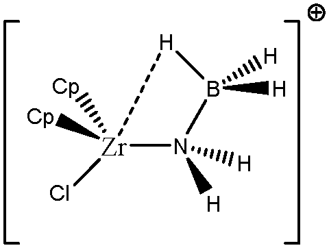
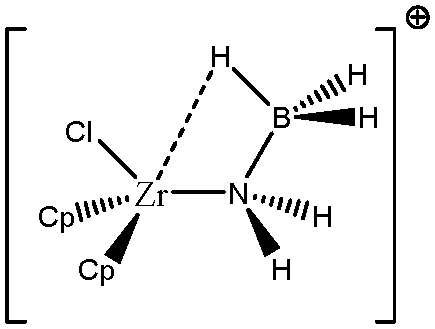

For all the amidoborane titanocene or zirconocene complexes, where the nitrogen atom is at the α-position and the boron atom at the β-position, the presence of a B–H protonated basin containing a metallic contribution ranging from 3% to 6% of the V(H) population is a clear indicator of the existence of a β-agostic bond. This is supported by the bond lengthening and frequency red-shift of the B–Hagostic bond. Compared to the C–H agostic bonding, the B–H agosticity should be considered as medium to strong interaction. This consideration is naturally in line with the decrease of the electron density at the B–Hagostic bond critical point. It is graphically evidenced on the linear regression graph (Table 9).
Globally, the ELF/QTAIM criteria led to a homogeneous and consistent description of the bonds thus supporting the use of “agostic” for both σ C–H⋯M and σ B–H⋯M intramolecular bonding.
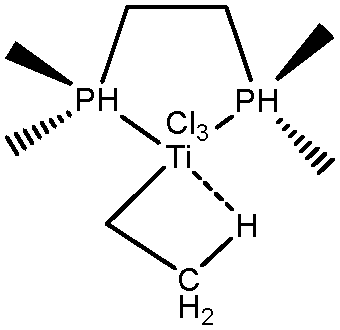
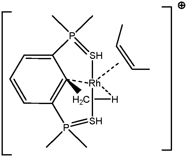
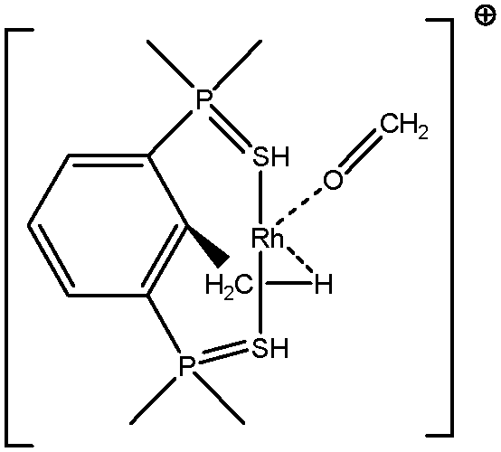
5. Parameters influencing the agostic character of bonding
To further investigate σ C–H β-agostic interactions and the parameters affecting such bonding, an interesting case-study of rhodium thiophosphoryl pincer investigated by Milstein et al. will be detailed below. Indeed, the authors reported the formation of identical agostic bonds with Rh that also interacts either with but-2-ene or with formaldehyde. The agostic hydrogen atoms are characterized by largely different geometrical parameters, and the topological investigation proves that the nature of the co-ligand R is of paramount importance on the agostic interaction (see Scheme 1).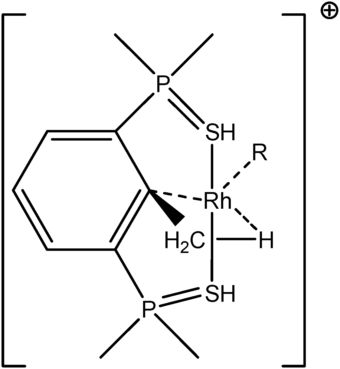 | ||
| Scheme 1 Rhodium thiophosphoryl pincer studied by Milstein et al., R = but-2-ene or formaldehyde.66 | ||
To better understand the co-ligand influence we will carefully analyze and compare the topological properties of the Rh-butene-Milstein compound to those of Rh-H2CO-Milstein. Tables 10 and 11 report the most relevant topological properties of both Rh-butene-Milstein and Rh-H2CO-Milstein complexes.
| H-agostic compound | QTAIM propertiesa | ELF propertiesb |
|---|---|---|
| a BCP and RCP are the bond and ring critical points corresponding to the (3, −1) and (3, +1) critical points. b V(X,Y) and V(X,Y,Z) stand for the disynaptic and trisynaptic basins which share two and three core basins, respectively. | ||
| Pincer (S-C-S)-R: R = cis-2-butene | BCP(Hβ, Rh): Yes | V(Rh, Cβ, Hβ): Yes |
| BCP(Cα, Rh): Yes | V(Rh, Cα): No | |
| BCP(Cβ, Rh): No | V(Rh, Cβ): No | |
| RCP(Rh, Hβ, Cβ, Cα): Yes | V(Cα, Cβ, Rh): Yes | |
| BCP(C(Ligand), Rh): Yes | V(C(Ligand), Rh): Yes | |
| BCP(C(Ligand), Rh): Yes | V(C(Ligand), Rh): Yes | |
| RCP(Rh, C, C): Yes | ||
| Pincer (S-C-S)-R: R = OCH2 | BCP(Hβ, Rh): Yes | V(Rh, Cβ, Hβ): Yes |
| BCP(Cα, Rh): No | V(Rh, Cα): No | |
| BCP(Cβ, Rh): No | V(Rh, Cβ): No | |
| RCP(Rh, Hβ, Cβ, Cα): No | V(Cα, Cβ, Rh): Yes | |
| BCP(O(Ligand), Rh): Yes | V1(O(Ligand), Rh): Yes | |
| V2(O(Ligand), Rh): No | ||
| Agostic compound | QTAIM propertiesaρ, ∇2ρ, H, ε | ELF propertiesb M, C and H contributions |
|---|---|---|
| a The four QTAIM characteristics at a critical point are given by ρ (the charge density), ∇2ρ (the Laplacian of charge density), H (the energy density) and ε (the ellipticity). Note that we have only the first three characteristics at a RCP. These quantities are given in atomic units. b The X/Y/Z contributions are the atomic contributions in the averaged population of the V(X,Y,Z) basin. These numbers are in electrons. | ||
|
Pincer (S-C-S)-R:
R = cis-2-butene Rh-butene-Milstein66 |
BCP(Hβ, Rh): 0.055; +0.204, −0.008, 0.29 | V(Rh, Cβ, Hβ): 0.05/1.02/0.95 |
| BCP(Cα, Rh): 0.050, +0.141, −0.008, 0.12 | V(Cα, Cβ, Rh): 1.25/0.91/0.06 | |
| RCP(Rh, Hβ, Cβ, Cα): 0.045, +0.172, −0.004, No ε | ||
| BCP(C(Ligand), Rh): 0.102, +0.192, −0.034, 1.13 | V(C(Ligand), Rh): 0.54/0.23 | |
| BCP(C(Ligand), Rh): 0.111, +0.158, −0.043, 0.37 | V(C(Ligand), Rh): 0.63/0.21 | |
| RCP(Rh, C, C): 0.100, +0.297, −0.027, No ε | ||
|
Pincer (S-C-S)-R:
R = OCH2 Rh-H2CO-Milstein66 |
BCP(Hβ, Rh): 0.107, +0.255, −0.046, 0.26 | V(Rh, Cβ, Hβ): 0.23/0.93/0.96 |
| V(Cα, Cβ, Rh): 1.24/0.99/0.09 | ||
| BCP(O(Ligand), Rh): 0.086, +0.488, −0.011, 0.46 | V1(O(Ligand), Rh): 2.31/0.03 | |
| V2(O(Ligand), Rh): 2.81/0.00 | ||
A close look of the data reported in Tables 10 and 11 allows us to summarize the similarities and differences between the titled complexes as follows:
• As it concerns the weak interactions, despite overall agreement between the topologies of ELF and QTAIM, few differences however have been underlined.49,75–78 Nevertheless, we would like to emphasize that we believe in the complementarity of these two methods, rather than mutual exclusion. But having said that, we remind the readers that there is no bond critical point between Hα and the metallic center, while we have a trisynaptic protonated basin accounting for the α-agostic interaction. Topological analysis of the C–C bonding – bond between the carbon of methyl and that of aryl – obtained from both QTAIM and ELF methods are likewise complementary and often clarify each other. In both Rh-butene-Milstein and Rh–H2CO–Milstein pincer complexes the C–C bond valence basin is indeed a trisynaptic basin with a non-negligible contribution from the metallic center (0.06 and 0.09 e−) which is a clear indication of the η3-C–C–H agostic compound. This conclusion supports the analysis advanced in the paper of Milstein and coworkers.66 As for the QTAIM analysis, it gives a BCP between the rhodium and the C atom of the aryl group in the case of the Milstein pincer bonded with cis-2-butene, while there exists no such a BCP for the other species. This means that the agostic interaction in the Rh-butene-Milstein could be referred to as the traditional β-agostic compound, while this is not the case for the Rh-H2CO-Milstein pincer complex.
• The ligand effect is another striking feature of these pincer-R (R = cis-2-butene or OCH2) agostic compounds. It is worth noting that both QTAIM and ELF topologies provide the same analysis for the ligand effect.
• In the case of the cis-2-butene ligand, rhodium thiophosphoryl pincer cation involves in the formation of two non-equivalent disynaptic basins labeled as V(C(Ligand), Rh) in Tables 10 and 11. The metal atom contribution amounts to 33% and 42% of the total averaged population of these metal–ligand bonds. These basins clearly are indicative of the formation of two metal–carbon coordinate covalent bonds. In parallel, we found two bond critical points for two Rh–C bonds and a RCP in the center of a C–Rh–C triangle. The non-negligible negative values of the energy density at the BCPs (−0.034 and −0.043) clearly indicate the non-negligible covalency of these bonds. As a consequence, the formation of these coordinate covalent bonds enriches the valence shell of the metal leading to lower acidity. Accordingly, the agostic interaction is relatively weak (as shown by values presented in Table 7, with a small covariance V(H)/C(M), and a small contribution of the metal in the valence basin of the agostic hydrogen atom). This weak agostic interaction is geometrically confirmed by a small Hagost–C distance and a large Hagost–Rh distance.
• Contrarily, in the case of the formaldehyde-rhodium thiophosphoryl pincer cation, the interaction between oxygen and rhodium atoms is almost weak – manifested by small contribution of Rh in the one of the two valence basins of oxygen – and thus without noticeable change in the valence shell of metal. Thus the electron-deficiency of the Rh center is not counterbalanced by a notable electron transfer. As a consequence, the agostic bonding between Rh and H will be enhanced. Geometrically, the Hagost–Rh distance will be smaller than in the previous case, and the Hagost–C distance will be larger, thus leading to a more pronounced activation of the H–C bond.
Thus, the presence of a co-ligand can be of paramount importance in the activation of a C–H bond by means of the formation of an agostic bond, and a topological description of the systems may help in understanding these differences.
On the other hand, a change in the nature of the co-ligand do not necessarily lead to a fundamental change in the agostic character of the bonding. As an example, Table 12 allows to follow the geometry and the topological characterization of the valence basin of the agostic hydrogen atom in β- and γ-agostic alkyl titanium complexes studied by Baird et al.64 The initial agostomers contain two cyclopentadienyl ligands. We suggest the substitution of a cyclopentadienyl ligand either by formaldehyde or by a chlorine atom to not lead to a huge distortion of the agostic bonding: Hagost–Ti and Hagost–C distances are almost unchanged (see Table 11). As far as the topological description of the valence basin of the agostic hydrogen atom is concerned, almost no change is observed, neither in the contribution of the metal center to the protonated valence basin nor in the covariance values. Thus, in this case, the substitution of the cyclopentadienyl ligand by formaldehyde or by a chlorine atom does not affect the agostic character of the bond.
| Isomer | Characterization |
|
|
|---|---|---|---|
| β | γ | ||
| R1 = R2 = Cp | V(H) | 1.93 | 1.95 |
| Ti/C/H | 0.06/0.77/1.10 | 0.05/0.81/1.09 | |
| Cov(V(H)/C(M)) | −0.08 | −0.07 | |
| d agosticTi–H (Å) | 2.09 | 2.00 | |
| d agosticH–C (Å) | 1.16 | 1.15 | |
|
R1 = Cp
R2 = OCH2 (TRANS) |
V(H) | 1.98 | 1.99 |
| Ti/C/H | 0.04/0.86/1.08 | 0.03/0.88/1.07 | |
| Cov(V(H)/C(M)) | −0.07 (AIM: −0.06) | −0.06 (AIM: −0.05) | |
| d agosticTi–H (Å) | 2.12 | 2.10 | |
| d agosticH–C (Å) | 1.13 | 1.12 | |
| R1 = R2 = OCH2 | V(H) | Starting from β isomer, it converges to γ agostomer. | 1.99 |
| Ti/C/H | 0.06/0.85/1.07 | ||
| Cov(V(H)/C(M)) | −0.09 (AIM: −0.07) | ||
| d agosticTi–H (Å) | 2.00 | ||
| d agosticH–C (Å) | 1.13 | ||
|
R1 = Cp
R2 = Cl (TRANS) |
V(H) | 1.98 | 1.97 |
| Ti/C/H | 0.08/0.80/1.09 | 0.06/0.84/1.08 | |
| Cov(V(H)/C(M)) | −0.09 (AIM: −0.07) | −0.08 (AIM: −0.06) | |
| d agosticTi–H (Å) | 2.06 | 2.01 | |
| d agosticH–C (Å) | 1.14 | 1.14 | |
| R1 = R2 = Cl | V(H) | Starting from β isomer, it converges to γ agostomer. | 1.98 |
| Ti/C/H | 0.08/0.84/1.06 | ||
| Cov(V(H)/C(M)) | −0.09 (AIM: −0.07) | ||
| d agosticTi–H (Å) | 1.99 | ||
| d agosticH–C (Å) | 1.15 | ||
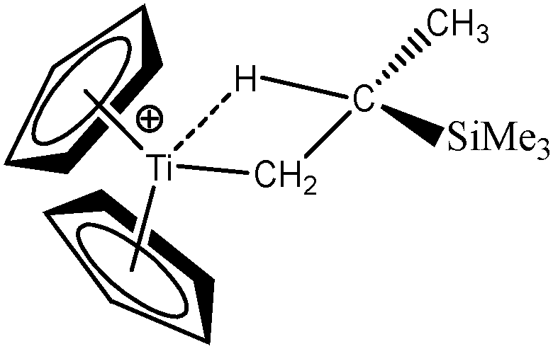
To further investigate the parameters influencing the formation of agostic bonds, we studied the influence of the metallic center on the agosticity. The β model compound of Popelier and Logothetis was chosen. Table 13 shows that the substitution of the titanium atom by either Zr or Hf does not affect the geometry of the agostic bond, and the topological description of the valence basin of the agostic hydrogen atom remains similar. Thus, in some cases, and specifically in the case of titanocene compounds, the substitution of the metallic center by an atom belonging to the same chemical family, does not affect the agostic character of the bond.
|
|
Topological description | ||
|---|---|---|---|
| β model compound (Popelier & Logothetis) | |||
| Geometry | ELF | AIM | |
| M = Ti | d(Hβ–Cβ) = 1.152 | V(Cβ–Hβ) = 1.93 | Q(Hβ) = −0.10 |
| d(M–Cα) = 2.010 | Ti(0.08)/C(0.75)/H(1.10) | Q(Ti) = +1.9 | |
| d(M–Cβ) = 2.393 | Cov(V(Hβ)/C(M)) = −0.10 | Cov(Ti/Hβ) = −0.08 | |
| d(M–Hβ) = 2.009 | |||
| a(M–Cα–Cβ) = 84.3 | |||
| a(Cα–Cβ–Hβ) = 113.5 | |||
| M = Zr | d(Hβ–Cβ) = 1.156 | V(Cβ–Hβ) = 1.94 | Q(Hβ) = −0.15 |
| d(M–Cα) = 2.148 | Zr(0.05)/C(0.74)/H(1.15) | Q(Zr) = +2.6 | |
| d(M–Cβ) = 2.553 | Cov(V(Hβ)/C(M)) = −0.10 | Cov(Zr/Hβ) = −0.08 | |
| d(M–Hβ) = 2.149 | |||
| a(M–Cα–Cβ) = 86.3 | |||
| a(Cα–Cβ–Hβ) = 113.9 | |||
| M = Hf | d(Hβ–Cβ) = 1.157 | V(Cβ–Hβ) = 1.93 | Q(Hβ) = −0.18 |
| d(M–Cα) = 2.140 | Hf(0.04)/C(0.71)/H(1.18) | Q(Hf) = +2.8 | |
| d(M–Cβ) = 2.545 | Cov(V(Hβ)/C(M)) = −0.09 | Cov(Hf/Hβ) = −0.07 | |
| d(M–Hβ) = 2.155 | |||
| a(M–Cα–Cβ) = 85.9 | |||
| a(Cα–Cβ–Hβ) = 114.5 | |||
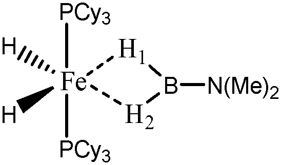
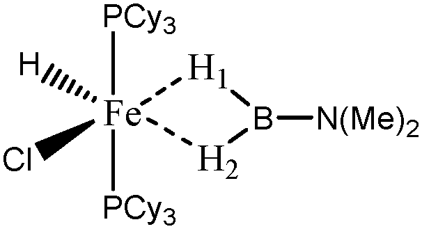
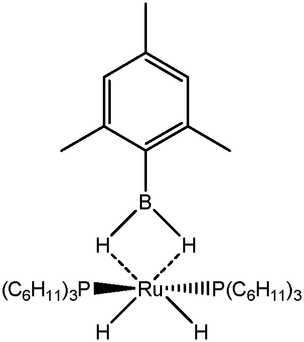
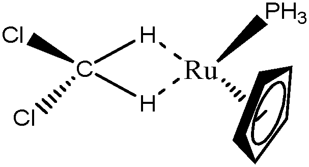
6. Characterization of double σ-BH2 and σ-CH2 interactions with a metallic center
The term “agostic bonding” was also used in the literature to describe situations in which a small molecule is in interaction with a metallic complex by means of two simultaneous weak interactions.26,69,70 Sabo-Etienne, Alcaraz et al. are particularly active in the study of such intermolecular interactions. To complete our topological study on agostic bonds, we applied our methodology to intermolecular interactions involving dimethylaminoborane69 and mesitylborane.70The complexes involved intermolecular interactions involving dimethylaminoborane and studied by Sabo-Etienne et al. are presented in Table 14.
|
|
||||
|---|---|---|---|---|
| Nature of M and X | Ru, H | Ru, Cl | Os, H | Os, Cl |
| d agosticH1–M (Å) | 1.85 | 1.62 | 1.81 | 1.62 |
| d agosticH1–B (Å) | 1.30 | 1.55 | 1.37 | 1.95 |
| d agosticH2–M (Å) | 1.85 | 2.00 | 1.81 | 1.97 |
| d agosticH2–B (Å) | 1.30 | 1.27 | 1.37 | 1.29 |
| Agostic character | Agostic | H1: strongly agostic | Agostic | H1: hydride |
| H2: weakly agostic | H2: agostic | |||
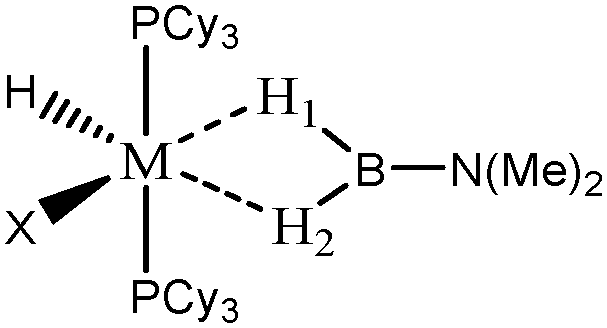
In the case of the osmium-containing complexes, an interaction is observed between the σ B–H bond and the metallic center when X = H. The substitution of this hydride by X = Cl dramatically affect the intermolecular interaction. The H atom trans to the chlorine atom leads to the formation of an hydride and the bond between H1 and B is broken. On the other hand the σ B–H agostic interaction with the metal is retained for the H2 atom.
In the case of the ruthenium-containing complexes, an interaction is similarly observed between the σ B–H bond and the metallic center when X = H. As in the case of the osmium-containing complex, the substitution of the X = H atom by a Cl atom causes a distinction between the H1 and H2 atoms: the H atom trans to the Cl atom leads to the formation of a stronger interaction with the metal, whereas the interaction between H2 and B becomes weaker.
For the present study, we selected the osmium-containing complexes for a topological investigation. Indeed, the two osmium-containing complexes allowed us to compare our quantitative approach with the strength of the interaction experimentally observed. Furthermore, these examples gave the opportunity that the topological descriptors herein chosen correctly discriminate a strong σ bond interaction and the formation of a hydride. For the sake of comparison, we also investigate the same system with M = Fe. Table 15 summarizes the topological data obtained for the intermolecular interactions of the four complexes.
| Compound |
|
|
|
|
|
|---|---|---|---|---|---|
| Os,H-MeB-Alcaraz69 | Os,Cl-MeB-Alcaraz69 | Fe,H-MeB | Fe,Cl-MeB | Ru,dimethyl amino-borane-Alcaraz70 | |
| V(H) | 2.25 | H1: 1.67 | 2.35 | H1: 2.32 | 2.16 |
| H2: 2.00 | H2: 2.28 | ||||
| M/B/H | 0.18/0.59/1.48 | H1: 0.39/0.01/1.27 | 0.30/0.54/1.51 | H1: 0.35/0.46/1.51 | 0.18/0.59/1.37 |
| H2: 0.04/0.42/1.54 | H2: 0.22/0.52/1.54 | ||||
| Cov(V(H)/C(M)) | −0.31 | H1: −0.40 | −0.31 | H1: −0.37 | −0.33 |
| H2: −0.17 | H2: −0.29 | ||||
| d agosticH1–M (Å) | 1.81 | 1.62 | 1.69 | 1.62 | 1.87 |
| d agosticH1–B (Å) | 1.37 | 1.95 | 1.27 | 1.29 | 1.28 |
| d agosticH2–M (Å) | 1.81 | 1.97 | 1.69 | 1.78 | 1.87 |
| d agosticH2–B (Å) | 1.37 | 1.29 | 1.27 | 1.24 | 1.28 |
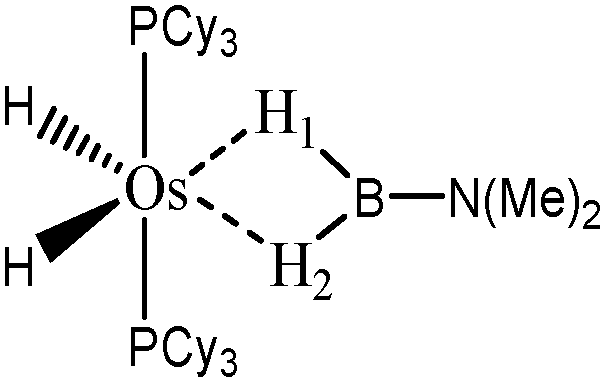

In the case of the osmium-containing complexes, the topological criteria selected for the present study are indeed consistent with the formation of an agostic bond, even if the total population of the valence basin of the hydrogen atom is a little bit high for a 3c–2e interaction.
As expected, H1 and H2 atoms are equivalent, and the agostic interaction is relatively strong compared with what was expected in the case of intramolecular interactions.
When the X = H atom is substituted by a chlorine atom, the topological description is fully consistent with what is expected from the data available in the literature. In the case of the H1 atom, the total population of the basin is 1.67 e− and the boron atom is not involved in this basin, which signifies that an hydride is formed, as already reported in the literature69 for this case. On the other hand, the topological description of the H2 atom is consistent with the formation of an agostic interaction. The total population of the valence basin of the hydrogen atom is 2.01 and both Os and B are involved in this basin. The covariance Cov(V(H)/C(M)) as well as the small contribution of the metal in the valence basin of H2 is clearly consistent with a weaker agostic interaction compared with what is observed for the complex with X = H.
Thus, the topological description herein proposed is qualitatively and quantitatively consistent with what is already reported for these osmium-containing complexes.
When the osmium atom is replaced by Fe, the total population of the valence basin of the hydrogen atoms interacting with the metallic center increases: a total population of 2.35 is calculated when X = H, whereas slightly smaller populations are obtained when X = Cl (2.33 and 2.29 e−).
For the “Fe,H-MeB” compound, both H1 and H2 atoms are identical, and the contribution of the metallic center to the valence basin of the hydrogen atom is quite large (0.30 e−), concomitantly with a large contribution of the boron atom (0.54). Furthermore, the covariance Cov(V(H)/C(M)) is large, thus suggesting that the agostic character of this compound is quite large.
When X = H is substituted by X = Cl, the two H1 and H2 atoms are characterized by quantitatively different interactions with the metallic center. Contrary to what was observed in the case of the osmium, the agostic interaction of the two H1 and H2 atoms is conserved. The agostic character of the hydrogen atom trans to the chloride atom is slightly reinforced, whereas the agostic character of the hydrogen atom cis to the chloride atom is slightly weakened.
In the case of a ruthenium-containing dimethylaminoborane compound,70 a similar topological description is calculated. Once again, the total population of the valence basin of the hydrogen atom is relatively high, but the contribution of the metallic atom in this basin and the covariance Cov(V(H)/C(M)) are fully consistent with the description of an agostic bond.
During the discussions it is clear that the chlorine substituted compounds lead to the formation of a hydridic bond only when the metallic atom is an osmium atom, whereas a strong agostic interaction is formed with iron and ruthenium atoms.
Thus, from a topological point of view, these intermolecular interactions are similar to the intramolecular, agostic interactions, and there is no topological reason for not using the same name, “agostic”.
In an attempt to better understand the formation of such intermolecular agostic bonds, model systems were studied:
(1) BH2Cl forming simultaneously two interactions with Ru(PH3)Cp,
(2) an isomer of the previous model system in which the BH2Cl molecule only forms one σ B–H interaction with the metallic center,
(3) an analog of the first model system in which BH2Cl is substituted by CH2Cl2. The formation of such complexes was proposed in the literature70,79 and was reported with Li as a metallic center,80 but not, to our knowledge, in the case of transition metal complexes. On the other hand, cases in which the three hydrogen atoms of a CH3–R group are simultaneously involved in agostic bonding with a same metallic center, were reported or proposed in the literature.81,82 Thus, a topological description of multiple σ C–H intermolecular agostic bonding is needed.
The topological criteria obtained for these three systems are presented in Table 16.
| Compound |
|
|
|
|---|---|---|---|
| Model system – 1 | Model system – 2 | Model system – 3 | |
| V(H) | 2.26 | 2.07 | 2.16 |
| M/B/H | 0.22/0.56/1.45 | 0.19/0.43/1.44 | 0.04/01.19/0.93 |
| Cov(V(H)/C(M)) | −0.41 | −0.35 | −0.14 |
| d agosticH–M (Å) | 1.73 | 1.73 | 2.03 |
| d agosticH–B or C (Å) | 1.34 | 1.35 | 1.12 |
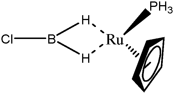
As already noted in the case of compounds reported in Table 15, relatively large values of total population of the hydrogen basins are observed in the case of the model systems 1 and 3. This corresponds to cases for which the molecule forms simultaneously two σ interactions with the metallic center. In the case of the Model system – 1, the topological criteria suggest the formation of two identical and relatively strong agostic bonds. A similar strong interaction is calculated in the isomeric system forming only one σ B–H interaction with the metallic center (Model system 2). On the other hand, in this case the total population of the valence basin is not particularly high, thus suggesting that the relatively large values of V(H) reported in Tables 15 and 16 are a specific signature of double intermolecular interactions.
In the case of the Model system – 3, both the hydrogen atoms involved in a σ interaction with the metallic center are identical. They are characterized by a lower total population of the valence basin of the hydrogen atoms, in comparison with the Model system – 1. Furthermore, the contribution of the metallic center in these valence basins is particularly weak. This may explain why the experimental formation, the isolation and the characterization of such systems may be difficult.
VI. Discussion
1. Identification of the existence or non-existence of agostic bonding
To begin with, Scheme 2 summarizes the conditions that should be fulfilled to conclude that an agostic bond exists between the C–H bond and the metallic center.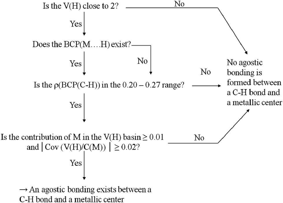 | ||
| Scheme 2 Determination of the existence or non-existence of an agostic bonding between a C–H bond and a metallic center. | ||
2. A qualitative comparison of different agostic bonds
To further evaluate the capability of the above presented statistical approach to qualitatively characterize the agostic bonding, our theoretical approach will be compared with experimental data. The first necessary step for such a comparison was obviously to find experimental criteria that correctly describe the agostic character of the bonding:• around different metallic centers,
• involving totally different compounds, and not focused in a well-defined chemical family of compounds,
• for α-, β-, γ-agostomers,
• involving σ C–H and σ B–H agostic bonds, with the possible presence of heteroatoms,
• with constrained geometries in the case of pincer ligands and bi-agostic compounds.
The experimental approaches generally used to characterize agostic bonds include NMR shifts, vibrational ν(C–H) shifts (IR spectroscopy) and X-ray structures.7,18–20,83 Obviously, the changes in reactivity due to the formation of an agostic bond, and more precisely the activation of the σ bond involved in the interaction with the metallic center, is in itself an evidence that such an interaction exists. More rarely EPR spectroscopy and visible/UV spectroscopy also proved, in some specific cases, to be able to describe the formation of an agostic bond.84,85
These methods will be shortly described below and in Table 17, in the context of the study of agostic bonding.
| Method | Effect leading to a possible characterization of an agostic bond | General values expected in the case of an agostic bond (and “normal” values expected for all other cases) | Limitations of the method |
|---|---|---|---|
| Reactivity | Activation of the C–H (or X–H, X = heteroatom such as B) bond. | Change in the reactivity.14,86 | The reactivity will obviously depend on co-ligands, geometry and the exact chemical nature of agostic bonding. |
| NMR | Redistribution of bonding-electron density in the formation of an agostic bonding. | δ = −5 to −15 ppm, 1JC–Hagostic = 75 to 100 Hz for C–H agostic bonding (1JCsp3–Hfree = 128 MHz)7,18,83,91 | NMR spectra cannot be obtained for dynamical systems. |
| Downfield paramagnetic shifts in the 700–1100 ppm range for axial ligands.92 | |||
| EPR spectroscopy | Influence on the Zeeman electronic effect of the distortion of the geometry. | Variations in the values of g's and determination of ΔH° and ΔS°.85,93 | Limited to paramagnetic compounds for with the single electron is involved in the agostic bonding. |
| IR spectroscopy | Weakening of the C–H bond leading to a reduction in frequency for ν(C–H) vibrational mode. | ν(C–H) = 2300–2700 cm−1 (to be compared with the ≈ 2700–3000 cm−1 range for free ligands).18–20 | Difficulty to identify a small weak signal that may overlap with other signals. |
| Visible/UV spectroscopy | Valence electron transition that may be affected by the formation of the M⋯H agostic bonding. | Depends on the crystal field perturbation induced by the agostic bonding.84 | Limited to cases for which the agostic bondings affect the color of the compound |
| X-ray diffraction | Geometrical distortion. | Distance Hagost–M = 1.8–2.3 Å (2.3–2.9 Å).7,94 | Difficulty to localize hydrogen atoms. Limited to agostomers that may be isolated as crystals. |
| Distance Hagost–X larger than the corresponding value for the free ligand | |||
| Change in the angles between the atoms.7 | |||
Experimentally, the formation of an agostic bond is distinguished first and foremost by an activation of the σ bond interacting with the metallic center.86 In the same chemical family of compounds, it may be possible to qualitatively estimate the agostic character of the bonding, by comparing their reactivity toward a same reagent. On the other hand, such a qualitative approach will be limited to a specific chemical family of compounds and may depend on the reagents. As a conclusion, such an approach, if fully relevant in a screening approach for the most suitable complex in a given reaction process, will not allow the determination of “absolute” agostic character of the bonding.
Spectroscopic methods that were applied to the study of agostic bonding almost cover the whole electromagnetic spectrum, from NMR to X ray spectroscopy.
The comparison of NMR shifts will not allow the comparison of agostic bonds of different chemical natures. Furthermore, only the strongest agostic bonding can be characterized by “classical” one-dimensional NMR experiments. Indeed, all the agostic bonds except the strongest ones are flexible in solution in the timescale of the NMR experiment, thus obscuring the effect.87,88
Complementarily to the NMR spectroscopy, EPR spectroscopy was also successfully applied for the characterization of agostic bonds.85 However, since this method is restricted to the study paramagnetic compounds, EPR spectroscopy is far from an “universal” experimental method that may be used to compare the agostic bonding of a wide set of complexes.
Another spectroscopic approach that was used to experimentally characterize agostic bonding is infrared (IR) spectroscopy.88 Once again, the characterization of weak interactions in mixtures that may contain agostic and anagostic isomers may be difficult. An elegant procedure to characterize agostic interactions by means of IR spectroscopy, particularly applied by Andrews et al.,89 consists of a coupling with the matrix isolation technique. Species to be analyzed are diluted in an inert medium in the gas phase, and further condensed on surface maintained at cryogenic temperatures. However, such a characterization is far from an easy tool that may be routinely used, without speaking about the experimental difficulty to generate a cryogenic matrix in which an agostic isomer is isolated. On the other hand, vibrational frequencies may be calculated by ab initio or DFT procedures once the geometry of the agostic compound is accurately determined.
Complexes of the transition metals are often colored. When the formation of an agostic bonding affects the energies of the d orbitals of the metallic center (especially the HOMO and the LUMO levels), visible/UV spectroscopy may be used to further characterize these interactions. Molybdenum β- and γ-agostomers were recently characterized by this technique.84 However the characterization of agostic bonds by visible/UV spectroscopy can only be applied in very specific cases for which the interactions between the metallic center and the σ bond affect the color of the species.
Since an agostic bonding should lead to a distortion of the geometry of a compound, the crystalline X-ray structure is an obvious characterization tool.90 The low scattering factor for hydrogen atoms and the difficulty to localize hydrogen in the vicinity of a metallic center are some of the limits of the method, in addition to the fact that agostic bonds may exist as intermediate species in liquid solution during reaction processes. In these latter cases, agostomers may not be obtained in the crystalline form. Even if limited to agostomers that may be isolated as crystals, and despite to its limitations X-ray diffraction structures were often reported in the literature for compounds involving agostic bonds. Furthermore, other experimental techniques provide data that may be further used for theoretical studies of the species. Thus geometries of agostomers can be obtained from DFT calculations and post-Hartree–Fock approaches. Theoretical calculations also allow the determination of spectroscopic data that may be compared with experimental values. It is then possible to determine structures for these compounds. From a geometrical point of view, the formation of an agostic bond will affect:
• the angles between the atoms,
• the Hagost–M distance,
• the Hagost–X distance.
The (harmonic) vibrational shift of the H–X stretching mode, Δω(H–X), caused by the agostic bonding, is an obvious tool to investigate the strength of the interaction. This shift is defined as follows:
| Δω(H–X) = ω(H–X)free ligand − ω(H–X)agostic compound |
The shift may depend on the nature of the X atom. In order to compare agostic bonds involving chemically different X atoms, we suggest the use of a normalized parameter:
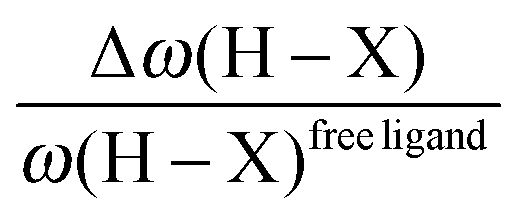
Additionally, geometrical parameters such as angles and distances were already proposed to characterize agostic bonds.7 The angles between the atoms will obviously depend on the system, and will not be directly linked to the agostic character of the bonding.
As already mentioned, the values of the angles cannot be used to compare the agostic character of bondings, in the set of compounds chosen for the present study, because their initial geometries are too much different from each other (Fig. 1). The Hagost–M distance will decrease, concomitantly with the increase in the Hagost–M distance, during the formation of an agostic bond. On the other hand, these two distances will be strongly affected by the nature of the X atom. In a first approximation, we can suggest that the ratio between dagosticH–X and dagosticH–M,  will not strongly depend on the nature of X.
Thus, two normalized experimental parameters may be used to compare the strength of agostic bonding,  and
and  . A simpler way to compare agostic bonding in a same family of complexes involving only one chemical type of H–X as agostic bond is to directly use the dagosticH–X and Δω(H–X) experimental parameters.
First of all, the contribution of the metallic center in the protonated agostic V(H) basin, MV(H), is an obvious important parameter.
On the other hand, this parameter depends on the whole structure of the metallic complex. As a consequence, a direct comparison of the MV(H) values will not allow the rigorous quantification of the agostic character of bonds. To overcome this limit, we propose to introduce a normalized parameter, the normalized metal contribution in the V(H) basin (NMV(H)). Its value is calculated by the ratio between the metal contribution in the V(H) basin and the total population of the V(H) basin:
 | (13) |
Fig. 4 shows the variations of MV(H) and NMV(H) as a function of the  ratio. The last point in the plots of the metal contribution corresponds to the hydride atom. This point was not included in the curve of the covariance. For all the other studied systems, all the values were taken into account in the plots.
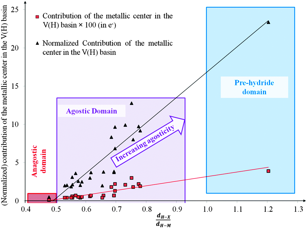 | ||
Fig. 4 Variation of the MV(H) and NMV(H) parameters as a function of the  ratio, with X = B or C, and ratio, with X = B or C, and 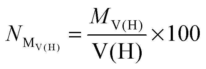 . . | ||
As already pointed out, the complexes selected for the present study cover a wide range of chemical families, owing to the nature of the metallic center, the nature of the ligand involved in the agostic bonding, the nature of co-ligands and the geometry of the complexes. Because of these chemical differences, a relative spread of the of the MV(H) and NMV(H) was expected. Given this point, a satisfactory linear correlation is observed for MV(H) and NMV(H) with the ratio of the distances. The coefficient of the linear regression clearly confirm that NMV(H) is a suitable criterion to compare agostic bonds in compounds belonging to different chemical families. Furthermore, the linear dependence observed demonstrates that NMV(H) can indeed be used to qualitatively characterize the agostic character of the bonding.
As mentioned earlier, the electron density at the bond critical point of the X–H bond is also an indication of the σ-donation to the metallic center and thus of the strength of the agostic bonding. Once again, if directly used, this parameter will depend on the system under investigation. As a consequence, the direct comparison of the ρ(BCPX–H) may be a suitable way to classify the strength of agostic bonds for a series of complexes belonging to a same chemical family of compounds, whereas the definition of a normalized value may be useful to compare agostic bonding in a set of complexes belonging to different chemical families. To this extent, we suggest to use the ratio between the ρ(BCP) for the X–H bond in the agostic complex and the ρ(BCP) for the X–H bond in the free ligand:

Fig. 5 illustrates the possibility of using:
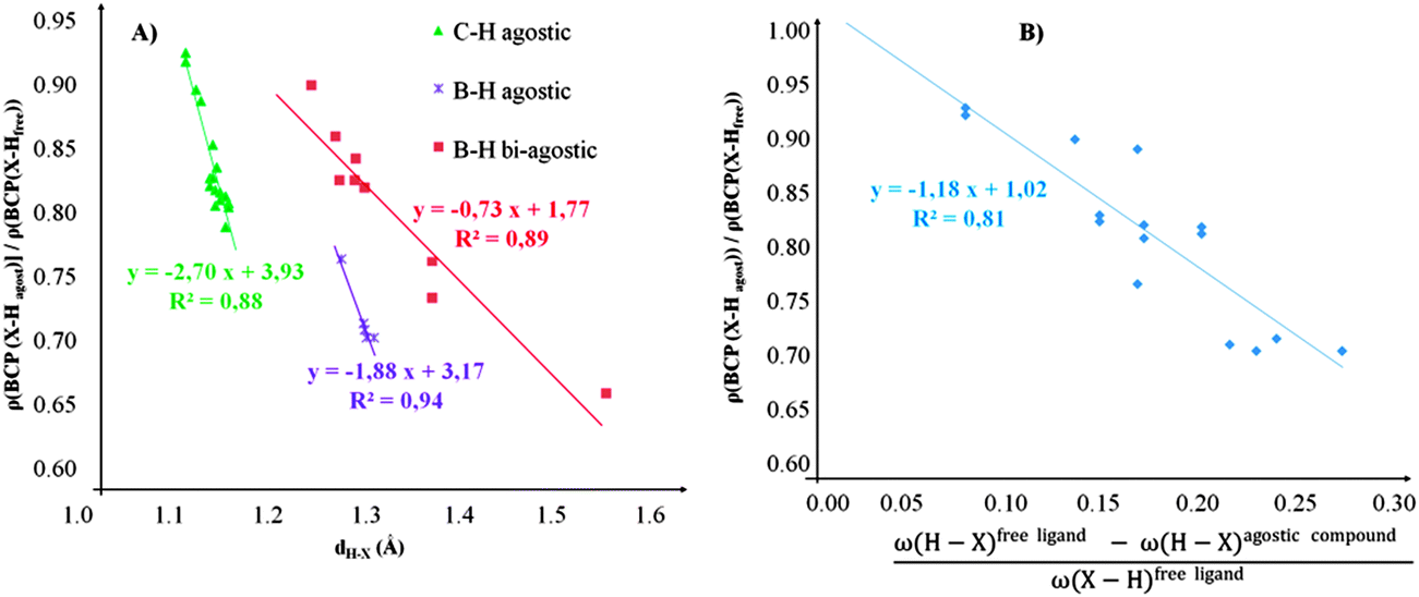 | ||
Fig. 5 Variation of the reduced  QTAIM parameter as a function of the: (A) dH–X distance, and (B) reduced frequencies of the H–X stretching mode. The strength of the agostic bonding increases from left to right and from top to bottom in both he graphs. QTAIM parameter as a function of the: (A) dH–X distance, and (B) reduced frequencies of the H–X stretching mode. The strength of the agostic bonding increases from left to right and from top to bottom in both he graphs. | ||
• direct H–X distances to characterize the strength of agostic bonds inside a same chemical family of compounds;
• reduced frequencies of the H–X stretching mode to characterize the strength of agostic bonds bonding in a set of complexes belonging to different chemical families;
• reduced ρ(BCP) for the H–X bond to classify the interaction with a metallic center.
Finally, the X–H bonds can be divided into four categories, depending on the strength of the M–H agostic bonding probably formed with a metallic center. Once the existence of the agostic bonding is ascertained based on the criteria presented in Scheme 2, four main estimators can be used to evaluate the strength of the interaction:
• two experimental parameters,  and
and 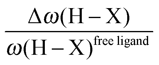 ; alternatively these parameters may be obtained by geometry optimization and theoretical calculations;
• the NMV(H) normalized parameter, based on ELF/QTAIM calculations;
• the  normalized QTAIM parameter.
In Table 18, a global classification is proposed to estimate the strength of an agostic bonding, based on these four parameters.
| Criterion | Characterization of the M–H interaction | |||
|---|---|---|---|---|
| Anagostic | Weak–medium agostic | Medium–strong agostic | Pre-hydride | |

|
<0.5 | 0.5–0.7 | 0.65–0.8 | >1 |
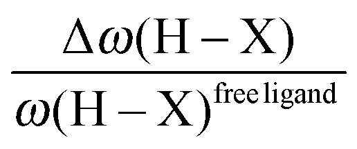
|
≥0.90 | 0.90–0.70 | <0.65 | |
| N MV(H) | <1 | 1–5 | 5–15 | >20 |
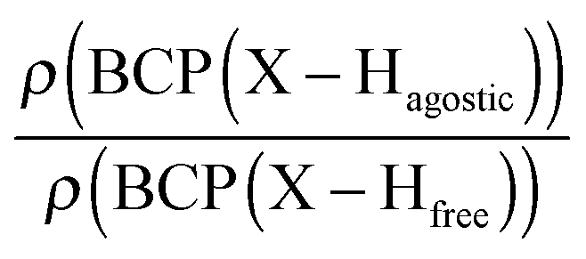
|
≥0.90 | 0.90–0.70 | <0.65 | |
VII. Conclusion
Herein we presented a topological quantitative investigation of σ C–H interactions. It was shown that the agostic character of the bonding can be compared even in the case of• complexes around a different metallic center,
• complexes containing different ligands and co-ligands,
• α-, β-, γ-, and η3-CCH agostomers,
• mono- and bis-agostic species,
• inter- and intramolecular agostic bonding.
Thus the present method makes it possible to compare the agostic character of interactions that take place in systems that do not belong to a same chemical family, by means of a simple topological approach. The large set of compounds presented in this article shows that the methodology proposed here can lead to an unambiguous determination of the agostic character, both qualitatively and quantitatively of a wide range of chemical compounds.
Furthermore, the topological description of intramolecular σ C–H and σ B–H interactions, as well as intermolecular σ B–H interactions, is similar, thus suggesting that the use of the same “agostic” term for all these interactions, is appropriate.
It has been evidenced that any X–H⋯M agostic bond could be fully analyzed using three topological descriptors obtained easily with the ELF method within the free TopMod code. We have to pay a particular attention on the stability and quality of the wave function derived from an optimization procedure. Indeed, the ELF topological analysis is actually an a posteriori approach whose reliability depends on that of the wave function in hand.
The most relevant descriptors are:
1. The existence of a protonated trisynaptic basin, labeled as V(Hag),
2. Three contributors participate in the averaged population of this basin: M/X/H,
3. The first and second descriptors are actually similar. We suggest them explicitly in order to underline the trisynaptic character of this basin which accounts for the 3c–2e interactions. Nevertheless, we also suggest the use of dimensionless descriptors to qualitatively estimate the strength of agostic bonding:
• the ratio between the metal contribution and the total population of the protonated basin, in order to emphasize the importance of the relative metal contribution. This  ratio allows the quantitative classification of the agostic character of bonding;
• the ratio of the electron densities at the BCP,  in order to take into account the weakening of the X–H bond due to the interaction with the metallic center.
4. We suggest the use of the above-mentioned descriptors in combination with two other criteria, ideally derived from experimental data. Indeed, experimental or, if not available, theoretical data, may be used to determine two additional reduced parameters that suitably describe the strength of agostic bonds:
• the weakening of the H–X bond due to the agostic interaction is characterized by a shift in the frequencies of the vibrational stretching mode of the H–X bond. The  reduced frequency parameter may be obtained from experimental IR spectra, or from (harmonic) calculations;
• the  reduced distance may be obtained or derived from X-ray structures. This reduced distance is increasing within the strength of the agostic bonding.
5. The covariance between two basins: the agostic protonated basin and the metallic core basin C(M). This quantity provide a measure of association between two quantities: C(M) and V(Hag). Agostic bonding for which the ratio NMV(H) is similar, the agostic character of the bonds increase with the |C(M)|.
Finally, we would like to emphasize the mutual complementary aspect of the topological results obtained from QTAIM and ELF analysis.
VIII. Computational details
The ELF calculations have been done using TopMod software.95 Furthermore, the AIMAll software was used for the quantitative study of the topological QTAIM data.96All the necessary wfn files for the topological investigations have been obtained using the Gaussian 09 Rev D.01 quantum chemical package. Calculations have been performed using different density functionals (B3LYP, PBE0 and TPSSh) as well as several basis sets (6-31++G(2d,2p), 6-311++G(2d,2p), TZVP, and LanL2DZ) as implemented in the Gaussian 09 package. In addition, the Def2-TZVP, Def2-TZVPD, LanL2TZ(P), and LanL2TZ(F) basis sets of Ahlrichs et al.,97 obtained from “EMSL Basis Set Exchange Library”.98 Furthermore, in order to take into account the dispersion contribution in some model compounds (mono- and bi-agostic model structures), geometry optimization have been done using the wB97XD range separated hybrid functional99 (Table 16) and also using the B2PLYPD3 double hybrid functional including the D3 version of Grimme's dispersion with the original D3 damping function.100 In order to ensure that an optimized structure corresponds to a true minimum, a frequency analysis was performed. Concerning the geometrical structures of the studied complexes, additional data on the optimized geometries are available in the ESI.†
Note added in proof
Since this work was submitted one paper dealing with the agostic-bonding in a particular set of pincer complexes has appeared.101 In this work several topological approaches have been used. Conclusions fully agree our description.References
- J. Chatt and J. M. J. Davidson, The tautomerism of arene and ditertiary phosphine complexes of ruthenium(0), and the preparation of new types of hydrido-complexes of ruthenium(II), J. Chem. Soc., 1965, 843–855 RSC.
- A. H. Janowicz and R. G. Bergman, Carbon–hydrogen activation in saturated hydrocarbons: direct observation of M + R–H → M(R)(H), J. Chem. Soc., 1982, 104, 352–354 CrossRef CAS.
- W. D. Jones, A. J. Vetter, D. D. Wick and T. O. Northcutt, Alkane Complexes as Intermediates in C–H Bond Activation Reactions, in Activation and Functionalization of C–H Bonds, ed. K. I. Goldberg and A. S. Goldman, ACS Symposium Series 885, Washington, DC, 2004, ch. 3, pp. 56–69 Search PubMed.
- M. Brookhart, M. L. H. Green and R. B. A. Pardy, Two-electron, three-centre carbon–hydrogen–cobalt bonds in the compounds [Co(η-C5Me4R)(η-C2H4)(η-C2H4-μ-H)]BF4, R = Me and Et, J. Chem. Soc., Chem. Commun., 1983, 691–693 RSC.
- M. Brookhart and M. L. H. Green, Carbon-hydrogen-transition metal bonds, J. Organomet. Chem., 1983, 250, 395–408 CrossRef CAS.
- M. Brookhart, M. L. H. Green and L. L. Wong, Carbon-Hydrogen-Transition Metal Bonds, Prog. Inorg. Chem., 1988, 36, 1–124 CrossRef CAS.
- M. Brookhart, M. L. H. Green and G. Parkin, Agostic interactions in transition metal compounds, Proc. Natl. Acad. Sci. U. S. A., 2007, 104, 6908–6914 CrossRef CAS PubMed.
- R. H. Crabtree, Organometallic alkane CH activation, J. Organomet. Chem., 2004, 689, 4083–4091 CrossRef CAS PubMed.
- B. Rybtchinsk, L. Konstantinovsky, L. J. W. Shimon, A. Vigalok and D. Milstein, Solvent-Stabilized Alkylrhodium(III) Hydride Complexes: A Special Mode of Reversible C–H Bond Elimination Involving an Agostic Intermediate, Chem. – Eur. J., 2000, 6, 3287–3291 CrossRef.
- I. Omae, Agostic bonds in cyclometallation, J. Org. Chem., 2011, 696, 1128–1145 CrossRef CAS PubMed.
- E. Clot, O. Eisenstein, T. Dubé, J. W. Faller and R. H. Crabtree, Interplay of Weak Interactions: An Iridium(III) System with an Agostic tert-Butyl but a Nonagostic Isopropyl Group, Organometallics, 2002, 21, 575–580 CrossRef CAS.
- T. Ziegler, The 1994 Alcan Award Lecture Density functional theory as a practical tool in studies of organometallic energetics and kinetics. Beating the heavy metal blues with DFT, Can. J. Chem., 1995, 73, 743–761 CrossRef CAS.
- H. H. Brintzinger, D. Fischer, R. MRlhaupt, B. Rieger and R. M. Waymouth, Stereospecific Olefin Polymerization with Chiral Metallocene Catalysts, Angew. Chem., Int. Ed. Engl., 1995, 34, 1143–1170 CrossRef CAS.
- M. Albrecht, Cyclometalation Using d-Block Transition Metals: Fundamental Aspects and Recent Trends, Chem. Rev., 2010, 110, 576–623 CrossRef CAS PubMed.
- J. Mathew, N. Koga and C. H. Suresh, C–H Bond Activation through σ-Bond Metathesis and Agostic Interactions: Deactivation Pathway of a Grubbs Second-Generation Catalyst, Organometallics, 2008, 27, 4666–4670 CrossRef CAS.
- M. Lein, J. A. Harison and A. J. Nielson, Identification of non-classical C–H⋯M interactions in early and late transition metal complexes containing the CH(ArO)3 ligand, Dalton Trans., 2013, 42, 10939–10951 RSC.
- F. Fuster and B. Silvi, Does the topological approach characterize the hydrogen bond?, Theor. Chem. Acc., 2000, 104, 13–21 CrossRef CAS.
- P. L. A. Popelier and G. Logothetis, Characterization of an agostic bond on the basis of the electron density, J. Organomet. Chem., 1998, 555, 101–111 CrossRef CAS.
- W. Scherer and G. S. McGrady, Agostic Interactions in d0 metal alkyl complexes, Angew. Chem., Int. Ed., 2004, 43, 1782–1806 CrossRef CAS PubMed.
- M. Lein, Characterization of agostic interactions in theory and computation, Coord. Chem. Rev., 2009, 253, 625–634 CrossRef CAS PubMed.
- M. Etienne and A. S. Weller, Intramolecular C-C agostic complexes: C-C sigma interactions by another name, Chem. Soc. Rev., 2014, 43, 242–259 RSC.
- W. H. Bernskoetter, C. K. Schauer, K. I. Goldberg and M. Brookhart, Characterization of a rhodium(I) σ-methane complex in solution, Science, 2009, 326, 553–556 CrossRef CAS PubMed.
- J. A. Calladine, S. B. Duckett, M. W. George, S. L. Matthews, R. N. Perutz, O. Torres and K. Q. Vuong, Manganese alkane complexes: an IR and NMR spectroscopic investigation, J. Am. Chem. Soc., 2011, 133, 2303–2310 CrossRef CAS PubMed.
- S. Lachaize and S. Sabo-Etienne, σ-Silane Ruthenium Complexes: The Crucial Role of Secondary Interactions, Eur. J. Inorg. Chem., 2006, 2115–2127 CrossRef CAS.
- G. Alcaraz and S. Sabo-Etienne, NMR: A good tool to ascertain σ-silane or σ-borane formulations?, Coord. Chem. Rev., 2008, 252, 2395–2409 CrossRef CAS PubMed.
- J. F. Hartwig, C. N. Muhoro and X. He, Catecholborane bound to titanocene. Unusual coordination of ligand σ bonds, J. Am. Chem. Soc., 1996, 118, 10936–10937 CrossRef CAS.
- A. T. Çolak, O. Z. Yeşilel and O. Büyükgüngör, A novel anagostic C single bond H⋯Cu interaction and clustered water molecules in copper(II)–pyridine-2,5-dicarboxylate complex, J. Mol. Struct., 2011, 991, 68–72 CrossRef PubMed.
- H. V. Huynh, L. R. Wong and P. S. Ng, Anagostic Interactions and Catalytic Activities of Sterically Bulky Benzannulated N-Heterocyclic Carbene Complexes of Nickel(II), Organometallics, 2008, 27, 2231–2237 CrossRef CAS.
- M. G. D. Holaday, G. Tarafdar, A. Kumar, M. L. P. Reddy and A. Srinivasan, Exploring anagostic interactions in 5,15-porphodimethene metal complexes, Dalton Trans., 2014, 43, 7699–7703 RSC.
- M. L. Yang, Y. A. Zhu, C. Fan, Z. J. Sui, D. Chen and X. G. Zhou, Density functional study of the chemisorption of C1, C2 and C3 intermediates in propane dissocuation on Pt(111), J. Mol. Catal. A: Chem., 2010, 321, 42–49 CrossRef CAS PubMed.
- G. Papoian, J. K. Nørskov and R. Hoffmann, A comparative theoretical study of the hydrogen, methyl, and ethyl chemisorption on the Pt(111) surface, J. Am. Chem. Soc., 2000, 122, 4129–4144 CrossRef CAS.
- T. Jacob and W. A. Goddard III, Agostic Interactions and Dissociation in the First Layer of Water on Pt(111), J. Am. Chem. Soc., 2004, 126, 9360–9368 CrossRef CAS PubMed.
- H. G. Cho, Agostic Structure of Titanium Methylidene Hydride (CH2
![[double bond, length as m-dash]](https://www.rsc.org/images/entities/char_e001.gif) TiH2): A Theoretical Investigation for the Elusive Intramolecular Interaction, Bull. Korean Chem. Soc., 2009, 30, 1631–1633 CrossRef CAS.
TiH2): A Theoretical Investigation for the Elusive Intramolecular Interaction, Bull. Korean Chem. Soc., 2009, 30, 1631–1633 CrossRef CAS. - S. Niu and M. B. Hall, Theoretical Studies on Reactions of Transition-Metal Complexes, Chem. Rev., 2000, 100, 353–406 CrossRef CAS PubMed.
- M. D. Su and S. Y. Chu, Theoretical Model for Insertion of the 16-Electron Species (η5-C5H5)M(L) into Saturated Hydrocarbons. A (η5-C5H5)M(CO) + CH4 (M = Ru–, Os–, Rh, Ir, Pd+, Pt+), Organometallics, 1997, 16, 1621–1627 CrossRef CAS.
- S. Zaric and M. B. Hall, Ab Initio Calculations of the Geometries and Bonding Energies of Alkane and Fluoroalkane Complexes with Tungsten Pentacarbonyl, J. Phys. Chem. A, 1997, 101, 4646–4652 CrossRef CAS.
- B. O. Roos, R. Lindh, H. G. Cho and L. Andrews, Agostic Interaction in the Methylidene Metal Dihydride Complexes H2MCH2 (M = Y, Zr, Nb, Mo, Ru, Th, or U), J. Phys. Chem. A, 2007, 111, 6420–6424 CrossRef CAS PubMed.
- E. D. Glendening, C. R. Landis and F. Weinhold, Natural bond orbital methods, Wiley Interdiscip. Rev.: Comput. Mol. Sci., 2012, 2, 1–42 CrossRef CAS.
- F. Weinhold and C. R. Landis, Natural bond orbitals and extensions of localized bonding concepts, Chem. Educ.: Res. Pract. Eur., 2001, 2, 91–104 RSC.
- F. Weinhold and C. R. Landis, Valency and Bonding – a natural bond donor-acceptor perspective, Cambridge University Press, 2005 Search PubMed.
- H. G. Cho and B. S. Cheong, Agostic Interaction of the Smallest Zirconium Methylidene Hydride: Reproduction of the Distorted Structure Experimentally Observed in Matrix Infrared Spectra, Bull. Korean Chem. Soc., 2009, 30, 470–481 Search PubMed.
- T. S. Thakur and G. R. Desiraju, Theoretical investigation of C–H⋯M interactions in organometallic complexes: A natural bond orbital (NBO) study, THEOCHEM, 2007, 810, 143–154 CrossRef CAS PubMed.
- M. Kaupp, The Unusual Fluxional Structure of Tetramethyloxotungsten: Quantum Chemical Structure Predictions for the d0 and d1 Complexes [MOR4] (M = W, Re; R = H, CH3), Chem. – Eur. J., 1998, 4, 2059–2071 CrossRef CAS.
- R. F. Bader, Atoms in Molecules: A Quantum Theory, Oxford University Press, Oxford, 1994 Search PubMed.
- S. Pillet, G. Wu, V. Kulsomphob, B. G. Harvey, R. D. Ernst and P. Coppens, Investigation of Zr-C, Zr-N, and Potential Agostic Interactions in an Organozirconium Complex by Experimental Electron Density Analysis, J. Am. Chem. Soc., 2003, 125, 1937–1949 CrossRef CAS PubMed.
- J. Saßmannshausen, Agostic or not? Detailed Density Functional Theory studies of the compounds, Dalton Trans., 2011, 40, 136–141 RSC.
- W. Scherer, V. Herz, A. Brück, C. Hau, F. Reiner, S. Altmannshofer, D. Leusser and D. Stalke, The Nature of β-Agostic Bonding in Late-Transition-Metal Alkyl Complexes, Angew. Chem., Int. Ed., 2011, 50, 2845–2849 CrossRef CAS PubMed.
- R. F. W. Bader and C. F. Matta, Bonding to titanium, Inorg. Chem., 2001, 40, 5603–5611 CrossRef CAS PubMed.
- V. Tognetti, L. Joubert, R. Raucoules, T. de Bruin and C. Adamo, Characterizing agosticity using the Quantum Theory of Atoms in Molecules: Bond Critical Poins and their local properties, J. Phys. Chem. A, 2012, 116, 5472–5479 CrossRef CAS PubMed.
- A. D. Becke and K. E. Edgecombe, A simple measure of electron localization in atomic and molecular system, J. Chem. Phys., 1990, 92, 5397–5403 CrossRef CAS PubMed.
- B. Silvi and A. Savin, Classification of chemical bonds based on topological analysis of electron localization functions, Nature, 1994, 371, 683–686 CrossRef CAS.
- A. Savin, B. Silvi and F. Colonna, Topological analysis of the electron localization function applied to delocalized bonds, Can. J. Chem., 1996, 74, 1088–1096 CrossRef CAS.
- B. Silvi, I. Fourré and M. E. Alikhani, The topological analysis of the electron localization function. A key for a position space representation of chemical bonds, Monatsh. Chem., 2005, 136, 855–858 CrossRef CAS PubMed.
- P. W. Ayers, Electron localization functions and local measures of the covariance, J. Chem. Sci., 2005, 117, 441–454 CrossRef CAS.
- S. Diner and P. Claverie, in Localization and Delocalization in Quantum Chemistry, ed. O. Chalvet, R. Daudel, S. Diner and R. Malrieu, Dordrecht, 1976, vol. II, pp. 395–448 Search PubMed.
- B. Silvi, The Spin-Pair Compositions as Local Indicators of the Nature of the Bonding, J. Phys. Chem. A, 2003, 107, 3081–3085 CrossRef CAS.
- S. Raub and G. Jansen, A quantitative measure of bond polarity from the electron localization function and the theory of atoms in molecules, Theor. Chem. Acc., 2001, 106, 223–232 CrossRef CAS.
- F. Fuster and S. Grabowski, Intramolecular hydrogen bonds: the QTAIM and ELF characteristics, J. Phys. Chem. A, 2011, 115, 10078–10086 CrossRef CAS PubMed.
- I. Fourré and J. Bergès, Structural and topological characterization of the three-electron bond: the SO radical, J. Phys. Chem. A, 2004, 108, 898–906 CrossRef.
- I. Fourré and B. Silvi, What can we learn from two-center three-electron bonding with the topological analysis of ELF?, Heteroat. Chem., 2007, 18, 135–160 CrossRef.
- J. Poater, M. Duran, M. Solà and B. Silvi, Theoretical evaluation of electron delocalization in aromatic molecules by means of Atoms in Molecules (AIM) and Electron Localization Function (ELF) topological approaches, Chem. Rev., 2005, 105, 3911–3947 CrossRef CAS PubMed.
- K. B. Wiberg, R. F. W. Bader and C. D. H. Lau, Theoretical analysis of hydrocarbon properties. 2. Additivity of group properties and the origin of strain energy, J. Am. Chem. Soc., 1987, 109, 1001–1012 CrossRef CAS.
- A. F. Dunlop-Brière, P. H. M. Budzelaar and M. C. Baird, α- and β-agostic alkyl-titanocene complexes, Organometallics, 2012, 31, 1591–1594 CrossRef.
- A. F. Dunlop-Brière, M. C. Baird and P. H. M. Budzelaar, [Cp2TiCH2CHMe(SiMe3)]+, an Alkyl–Titanium Complex Which (a) Exists in Equilibrium between a β-Agostic and a Lower Energy γ-Agostic Isomer and (b) Undergoes Hydrogen Atom Exchange between α-, β-, and γ-Sites via a Combination of Conventional β-Hydrogen Elimination–Reinsertion and a Nonconventional CH Bond Activation Process Which Involves Proton Tunnelling, J. Am. Chem. Soc., 2013, 135, 17514–17527 CrossRef PubMed.
- T. A. Atesin, T. Li, S. Lachaize, W. W. Brennessel, J. J. Garcia and W. D. Jones, Experimental and theoretical examination of C-CN and C-H bond activation of acetonitrile using zerovalent nickel, J. Am. Chem. Soc., 2007, 129, 7562–7569 CrossRef CAS PubMed.
- M. Montag, I. Efremenko, Y. Diskin-Posner, Y. Ben-David, J. M. L. Martin and D. Milstein, Exclusive C-C oxidative addition in a rhodium thiophosphoryl pincer complex and computational evidence for an η3-C-C-H agostic intermediate, Organometallics, 2012, 31, 505–512 CrossRef CAS.
- D. J. Wolstenholme, K. T. Traboulsee, A. Decken and G. S. McGrady, Structure and Bonding of Titanocene Amidoborane Complexes: A Common Bonding Motif with Their β-Agostic Organometallic Counterparts, Organometallics, 2010, 29, 5769–5772 CrossRef CAS.
- T. D. Forster, H. M. Tuononen, M. Parvez and R. Roesler, Characterization of β-B-Agostic Isomers in Zirconocene AmidoboraneComplexes, J. Am. Chem. Soc., 2009, 131, 6689–6691 CrossRef CAS PubMed.
- G. Bénac-Lestrille, U. Helmstedt, L. Vendier, G. Alcaraz and E. Clot, S. Sabo-Etienne. Dimethylaminoborane coordination to late transition metal centers: Snapshots of the B-H oxidative addition process, Inorg. Chem., 2011, 50, 11039–11045 CrossRef PubMed.
- G. Alcaraz, E. Clot, S. Sabo-Etienne, L. Vendier and U. Helmstedt, Mesitylborane as a bis (σ-B-H) ligand: an unprecedented bonding mode to a metal center, J. Am. Chem. Soc., 2007, 129, 8704–8705 CrossRef CAS PubMed.
- C. Adamo and V. Barone, Toward reliable density functional methods without adjustable parameters: The PBE0 model, J. Chem. Phys., 1999, 110, 6158–6169 CrossRef CAS PubMed.
- J. Tao, J. P. Perdew, V. N. Staroverov and G. E. Scuseria, Climbing the density functional ladder: nonempirical meta–generalized gradient approximation designed for molecules and solids, Phys. Rev. Lett., 2003, 146401, 1–4 Search PubMed.
- W. Scherer, D. J. Wolstenholme, V. Herz, G. Eickerling, A. Brück, P. Benndorf and P. W. Roesky, On the nature of agostic interaction in transition-metal amido complexes, Angew. Chem., Int. Ed., 2010, 49, 2242–2246 CrossRef CAS PubMed.
- U. Koch and P. L. A. Popelier, Characterization of C-H-O Hydrogen Bonds on the Basis of the Charge Density, J. Phys. Chem., 1995, 99, 9747–9754 CrossRef CAS.
- I. Vidal, S. Melchor, I. Alkorta, J. E lguero, M. R. Sundberg and J. A. Dobado, On the Existence of r-Agostic Bonds: Bonding Analyses of Titanium Alkyl Complexes, Organometallics, 2006, 25, 5638–5647 CrossRef CAS.
- B. Silvi, The synaptic order: a key concept to understand multicenter bonding, J. Mol. Struct., 2002, 614, 3–10 CrossRef CAS.
- N. Berkaïne, P. Reinhardt and M. E. Alikhani, Metal (Ti, Zr, Hf) insertion in the C–H bond of methane: manifestation of an agostic interaction, Chem. Phys., 2008, 343, 241–249 CrossRef PubMed.
- P. L. A. Popelier, On the full topology of the Laplacian of the electron density, Coord. Chem. Rev., 2000, 197, 169–189 CrossRef CAS.
- J. C. S. da Silva, W. B. de Almeida and W. R. Rocha, Theoretical investigation of the structure and nature of the interaction in metal-alkane σ-complexes of the type [M(CO)5(C2H6)] (M = Cr, Mo, and W), Chem. Phys., 2009, 365, 85–93 CrossRef CAS PubMed.
- D. Braga, F. Grepioni, K. Biradha and G. R. Desiraju, Agostic interactions in organic metal compounds. A Cambridge Structural database study, J. Chem. Soc., Dalton Trans., 1996, 3925–3930 RSC.
- J. Pinkas, V. Vargab, I. Cısarovac, J. Kubistaa, M. Horaceka and K. Mach, The first thermally stable half-sandwich titanium zwitterionic complex, J. Organomet. Chem., 2007, 692, 2064–2070 CrossRef CAS PubMed.
- W. E. Billups, S. C. Chang, R. H. Hauge and J. L. Margrave, Detection of a a-Complex in the Reaction of Cobalt Atoms with Methane, J. Am. Chem. Soc., 1993, 115, 2041–2042 CrossRef.
- R. H. Crabtree, The organometallic chemistry of the transition metals, John Wiley and Sons Inc, 5th edn, 2009, p. 307 Search PubMed.
- E. F. van der Eide, P. Yang and R. M. Bullock, Isolation of two agostic isomers of an organometallic cation: different structures and colors, Angew. Chem., 2013, 125, 10380–10384 CrossRef.
- W. W. Lukens, M. R. Smith III and R. A. Andersen, A π-Donor Spectrochemical Series for X in (Me5C5)2TiX, and β-Agostic Interactions in X Et and N(Me)Ph, J. Am. Chem. Soc., 1996, 118, 1719–1728 CrossRef CAS.
- See for instance: (a) R. S. Anju, D. K. Roy, B. Mondal, K. Yuvaraj, C. Arivazhagan, K. Saha, B. Varghese and S. Ghosh, Reactivity of Diruthenium and Dirhodium Analogues of Pentaborane – Agostic versus Boratrane Complexes, Angew. Chem., Int. Ed., 2014, 53, 2873–2877 CrossRef CAS PubMed; (b) M. A. Alvarez, D. Garcıa-Vivo, M. E. Garcıa, M. E. Martınez, A. Ramos and M. A. Ruiz, Reactivity of the r-Agostic Methyl Bridge in the Unsaturated Complex [Mo2(η5-C5H5)2(μ-η1:η2-CH3)(μ-PCy2)(CO)2]: Migratory Behavior and Methylidyne Derivatives, Organometallics, 2008, 27, 1973–1975 CrossRef.
- G. Alcaraz and S. Sabo-Etienne, NMR: a good tool to ascertain σ-silane or σ-borane formulations?, Coord. Chem. Rev., 2008, 252, 2395–2409 CrossRef CAS PubMed.
- See for instance (a) J. A. Calladine, S. B. Duckett, M. W. George, S. L. Matthews, R. N. Perutz, O. Torres and K. Q. Vuong, Manganese Alkane Complexes: An IR and NMR Spectroscopic Investigation, J. Am. Chem. Soc., 2011, 133, 2303–2310 CrossRef CAS PubMed; (b) O. Torres, J. A. Calladine, S. B. Duckett, M. W. George and R. N. Perutz, Detection of s-alkane complexes of manganese by NMR and IR spectroscopy in solution: (η5-C5H5)Mn(CO)2(ethane) and (η5-C5H5)-Mn(CO)2(isopentane), Chem. Sci., 2015, 6, 418–424 RSC.
- See for instance H. G. Cho, X. Wang and L. Andrews, The C–H Activation of Methane by Laser-Ablated Zirconium Atoms: CH2ZrH2, the Simplest Carbene Hydride Complex, Agostic Bonding, and (CH3)2ZrH2, J. Am. Chem. Soc., 2005, 127, 465–473 CrossRef CAS PubMed.
- See for instance F. M. Conroy-Lawis, L. Mole, A. D. Redhouse, S. A. Litster and J. L. Spencer, Synthesis of Coordinatively Unsaturated Diphosphine Nickel(II) and Palladium(II) β-Agostic Ethyl Cations: X-Ray Crystal Structure of [NiBut2P(CH2)2PBut2(C2H5)][BF4], J. Am. Chem. Soc., 1991, 1601–1603 Search PubMed.
- C. Elschenbroich, Organometallics: a concise introduction, Weinheim, New York, Basel, 2nd edn, 1992, p. 168 Search PubMed.
- K. Rachlewicz, S. L. Wang and C. H. Peng, C.H. Hung and L. Latos-Grazynski. Remarkable paramagnetically shifted 1H and 2H NMR spectra of Iron(II) complexes of 2-aza-21-carbaporphyrin: an evidence for agostic interaction, Inorg. Chem., 2003, 42, 7348–7350 CrossRef CAS PubMed.
- G. A. Luinstra, L. C. Ten Cate, H. J. Heeres, J. W. Pattiasina, A. Meetsmaand and J. H. Teuben, Synthesis and Reactivity of Tervalent Paramagnetic Titanium Compounds (η5-C5Me5)2TiR: Molecular Structure of (η5- C5Me5)2TiCH2CMe3, Organometallics, 1991, 10, 3227–3237 CrossRef CAS.
- T. S. Thakur and G. R. Desiraju, Misassigned C–HCu agostic interaction in a copper(II) ephedrine derivative is actually a weak, multicentred hydrogen bond, Chem. Commun., 2006, 552–554 RSC.
- S. Noury, X. Krokidis, F. Fuster and B. Silvi, Computational tools for the electron localization function topological analysis, Comput. Chem., 1999, 23, 597–604 CrossRef CAS.
- T. A. Keith, AIMAll (Version 14.10.27), TK Gristmill Software, Overland Park KS, USA, 2014 (http://aim.tkgristmill.com) Search PubMed.
- F. Weigend and R. Ahlrichs, Balanced basis sets of split valence, triple zeta valence and quadruple zeta valence quality for H to Rn: Design and assessment of accuracy, Phys. Chem. Chem. Phys., 2005, 7, 3297–3307 RSC.
- (a) D. Feller, The role of databases in support of computational chemistry calculations, J. Comput. Chem., 1996, 17, 1571–1586 CrossRef CAS; (b) K. L. Schuchardt, B. T. Didier, T. Elsethagen, L. Sun, V. Gurumoorthi, J. Chase, J. Li and T. L. Windus, Basis Set Exchange: A Community Database for Computational Sciences, J. Chem. Inf. Model., 2007, 47, 1045–1052 CrossRef CAS PubMed.
- J.-D. Chai and M. Head-Gordon, Long-range corrected hybrid density functionals with damped atom-atom dispersion corrections, Phys. Chem. Chem. Phys., 2008, 10, 6615–6620 RSC.
- L. Goerigk and S. Grimme, Efficient and Accurate Double-Hybrid-Meta-GGA Density Functionals—Evaluation with the Extended GMTKN30 Database for General Main Group Thermochemistry, Kinetics, and Noncovalent Interactions, J. Chem. Theory Comput., 2011, 7, 291–309 CrossRef CAS.
- C. Lepetit, J. Poater, M. E. Alikhani, B. Silvi, Y. Canac, J. Contreras-García, M. Solà and R. Chauvin, The Missing Entry in the Agostic–Anagostic Series: Rh(I)–η1-C Interactions in P(CH)P Pincer Complexes, Inorg. Chem. DOI:10.1021/acs.inorgchem.5b00069.
Footnote |
| † Electronic supplementary information (ESI) available. See DOI: 10.1039/c4cp05728g |
| This journal is © the Owner Societies 2015 |