Explicit solvent simulations of the aqueous oxidation potential and reorganization energy for neutral molecules: gas phase, linear solvent response, and non-linear response contributions†
Received
19th October 2014
, Accepted 8th April 2015
First published on 15th May 2015
Abstract
First principles simulations were used to predict aqueous one-electron oxidation potentials (Eox) and associated half-cell reorganization energies (λaq) for aniline, phenol, methoxybenzene, imidazole, and dimethylsulfide. We employed quantum mechanical/molecular mechanical (QM/MM) molecular dynamics (MD) simulations of the oxidized and reduced species in an explicit aqueous solvent, followed by EOM-IP-CCSD computations with effective fragment potentials for diabatic energy gaps of solvated clusters, and finally thermodynamic integration of the non-linear solvent response contribution using classical MD. A priori predicted Eox and λaq values exhibit mean absolute errors of 0.17 V and 0.06 eV, respectively, compared to experiment. We also disaggregate Eox into several well-defined free energy properties, including the gas phase adiabatic free energy of ionization (7.73 to 8.82 eV), the solvent-induced shift in the free energy of ionization due to linear solvent response (−2.01 to −2.73 eV), and the contribution from non-linear solvent response (−0.07 to −0.14 eV). The linear solvent response component is further apportioned into contributions from the solvent-induced shift in vertical ionization energy of the reduced species (ΔVIEaq) and the solvent-induced shift in negative vertical electron affinity of the ionized species (ΔNVEAaq). The simulated ΔVIEaq and ΔNVEAaq are found to contribute the principal sources of uncertainty in computational estimates of Eox and λaq. Trends in the magnitudes of disaggregated solvation properties are found to correlate with trends in structural and electronic features of the solute. Finally, conflicting approaches for evaluating the aqueous reorganization energy are contrasted and discussed, and concluding recommendations are given.
Introduction
Single electron transfer (SET) processes of organics in aqueous solution are important in biological,1 aquatic,2,3 and atmospheric chemistry.4,5 However, radicals are short-lived in aqueous solution, and accurate experimental measurements of single electron redox potentials are difficult, often requiring rapid spectroscopic methods.6 As a result, reliable single-electron oxidation potential data are limited for organic species in aqueous solution. This has motivated the development of computational methods to estimate accurate aqueous oxidation potentials for organic compounds7 and to improve our understanding of the chemical physics underlying the aqueous oxidation process.
We first briefly review the physical events taking place in a one-electron oxidation half-cell reaction. If SET occurs over a sufficiently large distance such that no charge-transfer complex is formed (outer sphere electron transfer), the half reaction of the electron donor (D) can be studied separately from the half reaction of the electron acceptor (A+):
In contrast to thermal SET reactions, here we partition the donor reaction (
eqn (1)) into an initial vertical electronic process followed by nuclear relaxation (
Fig. 1), comparable to photochemical experiments. This will allow a more direct link to the computational approach taken in the present work. The electronic transition and long-range solvent polarization happen on a much faster time frame (≤10
−15 s)
8,9 than the reorganization of the atomic nuclei of the extended solute + solvent system (≥10
−12 s),
10 and consequently the energies associated with each of these two processes can be considered separately. Thus, for the one-electron oxidation half-cell (
eqn (1)), the adiabatic free energy, AIE
aq, can be expressed as
15where VIE
aq is the vertical ionization energy of the reduced donor species (D), and
λaq is the half-cell reorganization energy of the donor (
Fig. 1). VIE
aq represents the fast electronic transition arising from the vertical oxidation of the reduced donor species and the associated electronic polarization of the solvent. The subsequent term, −
λaq, is the energy of relaxing the vertically oxidized donor and the proximate solvent, which are in the geometric configuration of the reduced donor system, to the equilibrium configuration of the oxidized donor system (D˙
+). Throughout this article, we will refer to
λaq determined
viaeqn (3) as the electrochemical definition of the reorganization energy.
12,15 Recent advances in aqueous liquid microjet spectroscopy have enabled the measurement of VIE
aq directly by experiment for soluble organic molecules.
9,11–14 Thus, in principle,
λaq can be determined from either measurements or computational estimates of both AIE
aq and VIE
aq, by
eqn (3). This contrasts with the definition that is employed in the Marcus linear response approximation, discussed further below.
 |
| | Fig. 1 Thermodynamic relationships between the adiabatic free energy of ionization, AIEaq, the vertical ionization energy (VIEaq), and the half-cell reorganization energy (λaq) in aqueous solution, for molecule D. The term rred denotes the reduced system geometry, and rox denotes the oxidized system geometry. The NVEAaq is defined by eqn (8). | |
Explicitly solvated molecular dynamics simulations can provide detailed insight into the influence of aqueous solvent on the oxidation potentials and reorganization energies of organic molecules. Early molecular dynamics approaches to model electron transfers were based on the work of Warshel,16–18 who originally employed classical Hamiltonians. Subsequently, density functional theory (DFT) and hybrid quantum-mechanical/molecular mechanical (QM/MM) Hamiltonians were used to simulate more accurate descriptions of the potential energy surface in solution.7,15,19–25 Recently, Ghosh et al. simulated the oxidation potentials of phenol and phenolate by using EOM-IP-CCSD26–31 to model the organic solute and using effective fragment potentials32,33 to model the solvent molecules, applying these methods to selected snapshots from a classical molecular dynamics trajectory of the explicitly solvated system.11 The simulation methods described above are computationally costly, and the results from finite simulation cells typically must be extrapolated to bulk solution. Alternatively, Eox values can be estimated more affordably with implicit solvent models, which treat solute–solvent interactions using empirically parameterized continuum dielectric models.1,34–50 We refer the reader to recent assessments of implicit solvent modeling approaches to estimate redox potentials.51,52
The linear response approximation (LRA) is widely employed for computational estimates of one-electron redox processes by explicit solvent simulation.11,15,19,22,23,53–61 The LRA is derived from the Marcus theory of electron transfer rates in solution.62–66 The LRA assumes that the polarization of the solvent is a linear function of the charge of the solute, and thus the solute's free energy of solvation is also a linear function of the solute charge at the solvent-accessible surface.15,65,67–70 These simplifications allow decreased computational expense of simulations of the one-electron oxidation potential. For example, under the LRA, the adiabatic free energy of the one-electron oxidation half-cell, AIELRAaq, can be computed from vertical gap quantities obtained from molecular dynamics simulations of an explicitly solvated system, as shown by Warshel,53 Kuharski et al.,54 Blumberger et al.,15,22,55–58 and others:11,19,23,59–61
| | | AIELRAaq = ½(VIEaq + NVEAaq) | (4) |
where NVEA
aq refers to the negative of the aqueous vertical electron affinity of the oxidized solute, D˙
+. NVEA
aq represents the energy required to remove one electron from a reduced donor system having the geometric configuration of the oxidized species system. By combining
eqn (3) and (4), the LRA also can be used to estimate the reorganization energy of the half-cell oxidation reaction, as
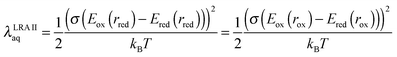
| | | λLRAaq = ½(VIEaq − NVEAaq) | (5) |
Use of the LRA thus enables straightforward computational protocols to estimate both the adiabatic free energy and the reorganization energy of the half-cell oxidation reaction, requiring only the determination of the vertical gap quantities, VIE
aq and NVEA
aq.
However the applicability of the linear response approximation depends on the system studied, and validity of the LRA is sometimes unclear. Comparison of the results obtained by the LRA and by thermodynamic integration provides a direct measure of the extent of non-linear response of the system. For example, Cheng et al. analyzed one-electron oxidations of benzoquinones, finding deviations of only 0.04–0.05 eV between the LRA result and the thermodynamic integration result for the free energy of oxidation of these neutral species.24 Sulpizi and Sprik used thermodynamic integration to analyze the deprotonation free energies of a set of organic and inorganic molecules in water, finding much larger non-linear response contributions of 0.25 to 0.90 eV for the neutral molecules studied.59 In another study, Blumberger and Sprik15 suggested possible deviation from linear solvent response for oxidation of Ag1+ to Ag2+ in aqueous solution, based on the finding that the vertical gap energy probability distributions were asymmetric for this oxidation half-cell. The LRA implies that the two vertical gap distributions should be symmetric, Gaussian-shaped, and of equal width.65 However in an additional investigation, thermodynamic integration of the Ag1+ to Ag2+ oxidation revealed only a 0.03 eV difference from the results obtained by free energy perturbation, indicating only a small contribution from non-linear solvent response.58 Later, Ayala and Sprik71 used thermodynamic integration to evaluate the non-linear response component for the oxidation of an M2+ to M3+ point charge model, finding very close agreement with the LRA result for this system. Further corroborating this result, histograms of the vertical energy gaps were found to fit a Gaussian distribution and were of the same width. However the LRA appeared less appropriate for the M1+ to M2+ oxidation process.71 Whereas histograms of vertical gaps from simulation data of the M1+ to M2+ oxidation process were Gaussian-shaped, the widths of the distributions were different (0.40 eV vs. 0.28 eV). Additionally, the radial distribution function indicated a change in the number of water molecules in the first solvation shell. These and other observations were suggestive of non-linear solvent response for the fictitious M1+/M2+ system. In other studies, diagnostics of the validity of the LRA have been less direct. For example, Ghosh et al. obtained reasonable agreement between computation and experiment for the oxidation potentials of phenol and phenolate, reporting errors of 0.28 and 0.18 V, respectively, using the LRA approach.11 They also found good agreement between simulated and experimental peak widths of aqueous photoelectron spectra for these two species. Thus only a handful of studies in the scientific literature have set out to evaluate the magnitude of non-linear solvent response in aqueous solution. Very few studies have investigated the extent of non-linear solvent response for the oxidation of neutral organics in aqueous solution.
The objectives of this study were as follows: (1) to formulate and validate an explicit solvent simulation protocol for estimating aqueous single electron oxidation potentials and half-cell reorganization energies, based on testing with structurally diverse neutral organic molecules; (2) to disaggregate and re-examine the free energy contributions to the aqueous oxidation potential and the reorganization energy that arise from the gas phase adiabatic ionization, the linear response of the solvent, and the non-linear solvent response; and (3) to identify the sources and magnitudes of error in the computed aqueous single electron oxidation potentials and aqueous reorganization energies, based on a systematic evaluation of each of several underlying thermodynamic sub-properties.
Methods
Theoretical approach
We first summarize the overall theoretical approach employed to compute the thermodynamic properties both in gas phase and in aqueous phase. The final computed estimates of each thermodynamic property are superscripted ref (“reference”) to distinguish them from intermediary computed quantities. An overview is provided in Scheme 1.
 |
| | Scheme 1 Overview of the disaggregated free energy properties that are used to construct the computed oxidation potential. | |
The gas phase adiabatic free energy of ionization of the reduced species at 298 K was determined as
| | | AIErefgas = Egas,ox(rox) − Egas,red(rred) + Gthermgas,ox(rox) − Gthermgas,red(rred) | (6) |
where
Egas,ox(
rox) is the electronic energy of the gas phase oxidized species in its stationary equilibrium geometry,
rox, and
Egas,red(
rred) is the free energy of the gas phase reduced species in its equilibrium geometry,
rred. Both energies were computed using high-level quantum chemistry methods. The terms
Gthermgas,ox(
rox) and
Gthermgas,red(
rred) include the zero-point vibrational energy and the thermal contributions to the free energy at 298 K arising from translations, rotations, and vibrations of the oxidized and reduced species, respectively. The gas phase vertical ionization energy of the reduced species at 298 K was determined as
| | VIErefgas = Egas,ox(rred) − Egas,red(rred) + ΔVIEvib![[thin space (1/6-em)]](https://www.rsc.org/images/entities/char_2009.gif) avggas(298 K) avggas(298 K) | (7) |
where
Egas,ox(
rred) is the electronic energy of the oxidized species in the stationary equilibrium geometry of the gas phase reduced species (
rred) and
Egas,red(
rred) is the electronic energy of the gas phase reduced species in its stationary equilibrium geometry (
rred), both computed using high-level quantum chemistry methods. ΔVIE
vibavggas is the difference in the vertical ionization energy between the vibrationally averaged structure at 298 K and the stationary structure. Analogous to the VIE
refgas, the negative of the vertical electron affinity of the oxidized species in gas phase at 298 K was determined as
| | | NVEArefgas = Egas,ox(rox) − Egas,red(rox) + ΔNVEAvibavggas(298 K) | (8) |
where
Egas,ox(
rox) is the electronic energy of the oxidized species in its stationary equilibrium geometry (
rox) and
Egas,red(
rox) is the electronic energy of the gas phase reduced species in the equilibrium geometry of the gas phase oxidized species (
rox). The gas phase half-cell reorganization energy of the reduced species was computed according to the electrochemical definition (
eqn (3)), as
| | | λrefgas = VIErefgas − AIErefgas | (9) |
Simulated aqueous properties were determined as follows. The aqueous vertical ionization energy of the reduced species at 298 K was determined as
| | | VIErefaq = VIErefgas + ΔVIEaq | (10) |
where VIE
refgas is the reference gas phase value determined by
eqn (7) and ΔVIE
aq represents the shift in the vertical ionization energy upon going from gas phase into aqueous solvent. The latter value was computed as
| | | ΔVIEaq = 〈VIEEOM-IP-CCSDaq〉 − VIEEOM-IP-CCSDgas | (11) |
where the term 〈VIE
EOM-IP-CCSDaq〉 represents a conformational average of the computed aqueous vertical ionization energy of an explicitly solvated reduced system, sampled using molecular dynamics. Vertical gap energies are computed with EOM-IP-CCSD to describe the solute and using effective fragment potentials (EFPs) to describe the solvent. The same level of theory is employed for the gas phase term in
eqn (11), VIE
EOM-IP-CCSDgas. Similarly, we determined the aqueous negative vertical electron affinity of the oxidized species as
| | | NVEArefaq = NVEArefgas + ΔNVEAaq | (12) |
and
| | | ΔNVEAaq = 〈NVEAEOM-IP-CCSDaq〉 − NVEAEOM-IP-CCSDgas | (13) |
where 〈NVEA
EOM-IP-CCSDaq〉 represents a conformational average of the computed aqueous negative vertical electron affinity of the explicitly solvated oxidized system. The terms in
eqn (13) are determined with the same computational protocols used for
eqn (11).
The aqueous adiabatic free energy of the one-electron oxidation half-cell reaction was determined in two different ways: by following the LRA approach (eqn (4)) and also by an extended approach intended to recover the effects of non-linear response. The LRA estimate was computed as
| | | AIELRAaq = ½(VIErefaq + NVEArefaq) | (14) |
where the values for VIE
refaq and NVEA
refaq are determined by
eqn (10) and (12), respectively. We repartitioned the vertical gap terms in
eqn (14) into a gas phase component and a solution phase contribution:
| | | AIELRAaq = AIELRAgas + ΔΔGLRAsolv | (15) |
By inspection of
eqn (10), (12) and (14), we can assign the gas phase term and the solution phase term in
eqn (15) as
| | | AIELRAgas = ½(VIErefgas + NVEArefgas) | (16) |
| | | ΔΔGLRAsolv = ½(ΔVIEcompaq + ΔNVEAcompaq) | (17) |
where AIE
LRAgas is the linear response approximation of the gas phase adiabatic free energy of ionization and ΔΔ
GLRAsolv is the linear solvent response contribution to the AIE
LRAaq.
A more complete estimate of AIEaq is obtained by including the appropriate non-LRA terms in both gas phase and solution phase, as follows:
| | | AIErefaq = AIErefgas + ΔΔGsolv | (18) |
where AIE
refgas is the gas phase adiabatic free energy of ionization given by
eqn (6). ΔΔ
Gsolv is the shift in the AIE upon moving from gas phase into aqueous solution, representing the change in the solvation free energy of the solute upon ionization. The term ΔΔ
Gsolv was computed as
| | | ΔΔGsolv = ΔΔGLRAsolv + ΔΔΔGnon-LRsolv | (19) |
where ΔΔ
GLRAsolv is the linear solvent response contribution, given by
eqn (17), and ΔΔΔ
Gnon-LRsolv represents the magnitude of non-linear solvent response upon ionization, as determined by classical molecular dynamics simulations.
The aqueous reorganization energy was computed according to the electrochemical definition:
| | | λrefaq = VIErefaq − AIErefaq | (20) |
where VIE
refaq was determined by
eqn (10), and AIE
refaq was determined by
eqn (18). We also determined an LRA estimate of the reorganization energy, given by
| | | λLRAaq = ½(VIErefaq − NVEArefaq) | (21) |
By consideration of
eqn (3) and (4),
eqn (21) can be equivalently written as
| | | λLRAaq = VIErefaq − AIELRAaq | (22) |
which is the LRA analogy to
eqn (20). Thus the half-cell electrochemical reorganization energy can be determined by completing the thermodynamic cycle (
Fig. 1), independent of the presence (or absence) of non-linear solvent response.
Finally, the oxidation potential of the half-cell reaction was estimated by the relationship
| | 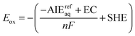 | (23) |
where
n is the number of electrons transferred (one),
F is the Faraday constant (96485.3365 C mol
−1, or 1 eV V
−1),
72 and SHE is the potential of the standard hydrogen electrode, 4.28 V.
73 The term EC is the integrated heat capacity of the electron according to Fermi–Dirac statistics, 0.03261 eV.
74 The EC term is needed to convert computed AIE
refaq values from the ion convention to electron convention.
74 The free energy of the gas phase free electron is zero under the ion convention, employed for reported AIE
refaq values. According to
eqn (23), our reported computational estimates of the oxidation potential employ the electron convention, enabling proper comparisons with reported experimentally measured
Eox data.
Chemical test set
The test set consisted of aniline, methoxybenzene, dimethylsulfide (DMS), imidazole, and phenol. These compounds were chosen because they represent diverse chemical structures for which experimental aqueous vertical ionization energy, experimental aqueous single electron oxidation potential data from pulse radiolysis, and/or experimentally derived reorganization energy data are available. Phenol has been known to undergo hydrogen atom transfer, a form of proton-coupled electron transfer (PCET), and thus its electron transfer may be better described by the bond dissociation free energy.75 However, the experimental BDFE of phenol is determined from the oxidation potential of phenol and the pKa of the oxidized phenol radical cation (or alternatively from the pKa of phenol and the oxidation potential of phenolate anion). The single electron oxidation potential of phenol cannot be measured directly, since the phenol radical cation is very acidic (pKa = −2)2 and thus undergoes rapid deprotonation. The experimental Eox value of phenol used in this study (Table 1) is based on the determination of the oxidation potential of phenolate, the pKa of phenol, and the pKa of phenol radical cation.2
Table 1 Experimental and computed thermodynamic data for the single-electron oxidation of organic compounds. All values are listed in eV at 298 K except Eox values, which are reported in V vs. SHE
| |
Aniline |
Methoxybenzene |
DMS |
Imidazole |
Phenol |
MUE |
Max. dev. |
|
Experimental and computed data reported in Tentscher et al.12λrefgas is determined by eqn (9).
Computed gas phase negative vertical electron affinity as defined by eqn (8).
Computed aqueous vertical ionization energy and aqueous negative vertical electron affinity as defined in eqn (10)–(13).
Computed free energy of oxidation from simulations, according to eqn (18).
AIEexptaq values are based on aqueous single-electron Eox data from pulse radiolysis.2,111–114
Computed free energy of oxidation under the linear response approximation according to eqn (14).
Computed aqueous reorganization energy as determined by eqn (20).
Computed aqueous reorganization energy according to the LRA, as determined by eqn (21).
Computed aqueous single electron oxidation potential as determined from simulation AIErefaq data, using eqn (23).
Computed aqueous single electron oxidation potential as determined from eqn (23) using AIErefgas and ΔΔGSMDsolv computed by SMD119/M06-2X120/aug-cc-pVTZ.
|
| AIErefgasa |
7.73 |
8.23 |
8.65 |
8.82 |
8.52 |
|
|
| VIErefgasa |
8.04 |
8.47 |
8.80 |
9.11 |
8.75 |
|
|
| NVEArefgasb |
7.52 |
8.03 |
8.70 |
8.61 |
8.33 |
|
|
|
λ
refgasa |
0.31 |
0.23 |
0.16 |
0.29 |
0.23 |
|
|
|
|
| VIErefaqc |
7.31 |
8.11 |
8.27 |
8.45 |
8.09 |
0.16 |
0.25 |
| VIEexptaqa |
7.49 |
|
|
8.51 |
7.84 |
|
|
| NVEArefaqc |
3.33 |
4.37 |
3.92 |
3.81 |
4.19 |
|
|
|
|
| AIErefaqd |
5.19 |
6.15 |
5.86 |
6.00 |
6.01 |
0.17 |
0.28 |
| AIEexptaqe |
5.27 |
5.87 |
5.91 |
|
5.75 |
|
|
| AIELRAaqf |
5.32 |
6.24 |
6.10 |
6.13 |
6.14 |
0.25 |
0.39 |
|
|
|
λ
refaqg |
2.12 |
1.95 |
2.41 |
2.45 |
2.08 |
0.06 |
0.10 |
|
λ
exptaqa |
2.22 |
|
|
|
2.09 |
|
|
|
λ
LRAaqh |
1.99 |
1.87 |
2.18 |
2.32 |
1.95 |
0.19 |
0.23 |
|
|
|
E
refoxi |
0.94 |
1.90 |
1.61 |
1.75 |
1.76 |
0.17 |
0.28 |
|
E
exptox
|
1.02 |
1.62 |
1.66 |
|
1.50 |
|
|
|
E
LRAox
|
1.07 |
1.99 |
1.85 |
1.8 |
1.89 |
0.25 |
0.39 |
|
E
SMDoxj |
1.18 |
1.82 |
1.85 |
1.91 |
1.92 |
0.24 |
0.42 |
Determination of AIErefgas, VIErefgas, and NVEArefgas values
For each compound in the test set, we used modified W1 methods to compute the gas phase adiabatic ionization energy, AIErefgas, and the vertical ionization energy of the reduced species, VIErefgas, obtained in our recent report.12 We also computed the gas phase negative vertical electron affinity of the oxidized radical species, NVEArefgas, following the same protocol as for the other two properties. Details of these computational procedures are described in ESI.† Briefly, equilibrium gas phase geometries were minimized with B2PLYP-D,76,77 using Ahlrich's tzvpp basis set78 augmented with diffuse functions from Dunning's aug-cc-pVTZ basis set for N, O, and S atoms, with the Gaussian09 rev. B.01 software suite79 with thermal contributions from computations of vibrationally averaged structures, according to the anharmonic VPT2 protocol.80
MM and QM/MM molecular dynamics simulations
Fully classical MM simulations were performed to generate initial solvated system structures for QM/MM simulations and also to conduct classical thermodynamic integration calculations. The parameters and computational methodologies for executing both the MM and QM/MM molecular dynamics simulations are described in ESI.† Briefly, gas phase geometries were optimized and RESP81 charges generated using M05-2X82/aug-cc-pVDZ83 as implemented in Gaussian09 rev. B.01.79 Solutes were solvated in AMBER (v. 11)84 whereby GAFF force field parameters85 were generated for the solute, and POL386 water molecules were used for the solvent using the SHAKE87 algorithm. We performed molecular dynamics trajectories of the solvated molecule using QM/MM88,89 molecular dynamics with the CP2K v. 2.2.422 software.90 The solute was represented quantum mechanically using BLYP-D291/TZV2P-GTH.92,93 The QUICKSTEP algorithm was used for the QM subsystem,94 with orbital transformation95 applied. For open shell species, restricted open-shell Kohn–Sham (ROKS) and self-interaction correction (SIC)96 with values of a = 0.2 and b = 0.0 were applied. Periodic boundary conditions (PBC) were maintained with the Ewald Poisson solver.97,98 Temperature in each of the QM and MM regions was maintained at 300 K using a three-chain Nosé–Hoover thermostat.99
Determination of ΔVIEaq and ΔNVEAaq values using solvated cluster snapshots from the QM/MM trajectory
The solvent-induced shifts in the vertical gap energies, ΔVIEaq and ΔNVEAaq (eqn (11) and (13)), were determined using solvated clusters, or “cluster snapshots”, extracted from instantaneous geometric configurations of the QM/MM molecular dynamics trajectories of the reduced and oxidized species, respectively. Each solvated cluster consisted of the solute and the 3072 water molecules that lay nearest to any point of the van der Waals surface of each solute. Individual clusters were extracted at equally spaced time intervals (250 fs each) of the 25 ps QM/MM production trajectory. On each extracted cluster, the vertical gap energy was computed using EOM-IP-CCSD26–31/6-31+G(d)100–103 to describe the solute electronic structure and effective fragment potentials (EFPs)32,33,104 to describe the water molecules, as implemented in QCHEM v. 4.01.0.105 The one-electron terms for Coulomb, self-consistently computed polarization, exchange-repulsion, and dispersion106 interactions contribute to the total QM-EFP interaction energy of the system. In order to superimpose the fixed geometry EFP water molecules onto the coordinates of the (also fixed geometry) POL3 water molecules of the QM/MM trajectory, we minimized the squared deviation of absolute coordinates of all three centers for each water molecule in the cluster.
For the reduced species, the ΔVIEaq value was determined as the averaged computed vertical ionization energy of all solvated clusters, 〈VIEEOM-IP-CCSDaq〉, minus the gas phase vertical ionization energy computed at the same level of theory, VIEEOM-IP-CCSDgas (eqn (11)). The VIEEOM-IP-CCSDgas was determined by eqn (7), where the gas phase energy gaps Egas,ox(rred) and Egas,red(rred) were computed with EOM-IP-CCSD/6-31+G(d). The difference between the vertical ionization energy of the vibrationally averaged gas phase solute geometry and that of its stationary geometry, ΔVIEEOM-IP-CCSD,vibavggas, was also computed with EOM-IP-CCSD/6-31+G(d) (Table S1, ESI†). The ΔNVEAaq value of the oxidized species was computed with an analogous protocol (eqn (13)). Tentscher et al. employed this same computational protocol recently for the simulation of aqueous vertical ionization energies.12 The approach described above is also similar (although not identical) to the protocol employed by Ghosh et al. for the aqueous simulation of vertical ionization energy of phenol and the vertical electron affinity of the oxidized phenol radical cation.11 By computing the vertical gap energies on large gas phase clusters rather than on periodic systems, we avoid having to determine the Poisson potential shift71,107–109 that arises from the background counter-charge applied to systems having a net non-zero charge. Previous work has shown that correcting for the Poisson potential shift is not trivial.19,20,110
Computation of contributions from non-linear solvent response, ΔΔΔGnon-LRsolv
We accounted for non-linear solvent response contributions to the change in solvation free energy upon one-electron oxidation, ΔΔΔGnon-LRsolv, using classical simulations. This term was determined as the difference between the adiabatic free energy of the one-electron oxidation value computed by thermodynamic integration, AIETIaq (which includes nonlinear solvent response), and that computed using free energy perturbation, AIEFEPaq (which assumes only linear solvent response), using a classical Hamiltonian in both cases.| | | ΔΔΔGnon-LRsolv = AIETIaq − AIEFEPaq | (24) |
See ESI† for further details about the computational methodology employed for eqn (24).
Results and discussion
We analyzed both simulated and experimental data to determine the disaggregated thermodynamic contributions underlying the half-cell oxidation potential (Eox) and the half-cell reorganization energy (λaq) in water, for several neutral organic solutes. We first report the adiabatic ionization energy and vertical gap energies in gas phase (AIErefgas, VIErefgas, and NVEArefgas). This allows us to isolate the influence of aqueous solvent on the oxidation process. We then discuss the shifts in the vertical gap energies upon moving from gas phase into aqueous solution, ΔVIEaq and ΔNVEAaq, which together determine the linear solvent response contribution, ΔΔGLRAsolv (eqn (17)). Under the linear response approximation, the aqueous vertical gap energies VIEaq and NVEAaq together dictate the magnitudes of both the adiabatic free energy (AIELRAaq) and the reorganization energy (λLRAaq) of the half-cell oxidation process (eqn (4) and (5)). We then move beyond the LRA and examine the role of non-linear solvent effects (ΔΔΔGnon-LRsolv). These separated thermodynamic components illuminate several distinct physical contributions to the aqueous half-cell oxidation potential. Finally, we discuss the first reported comparison of simulated and experimentally derived half-cell reorganization energies for several organic molecules in aqueous solution, including a re-examination of the LRA and contributions beyond linear response.
Gas phase ionization properties: AIErefgas, VIErefgas, NVEArefgas, and λrefgas
We computed high-quality gas phase values for the adiabatic ionization energy of the reduced species (AIErefgas), vertical ionization energy of the reduced species (VIErefgas), negative vertical electron affinity of the oxidized species (NVEArefgas), and reorganization energy of the reduced species (λrefgas) for each compound in the test set (Table 1). For the five compounds studied here, VIErefgas values ranged from 8.04 to 9.11 eV. The vertical ionization energies of the reduced species uniformly exhibited the highest energies compared to the other three properties. NVEArefgas values were consistently lower than VIErefgas, differing by −0.11 eV (DMS) to −0.51 eV (aniline). AIErefgas values fell in between the two vertical properties, with the exception of DMS, which exhibited an AIErefgas value of 8.65 eV and a slightly higher NVEArefgas value of 8.70 eV, due to differences in vibrational contributions. These reported values of AIErefgas, VIErefgas, and NVEArefgas indicate that substantial energy is required for the gas phase one-electron oxidation of the molecules investigated here, irrespective of whether it is a vertical or adiabatic process. This arises largely from the electronic contribution to ionization. Vibrational and rotational contributions to AIErefgas, VIErefgas, and NVEArefgas at 298 K are small: computed ΔGthermgas,ox contributions were ≤0.11 eV for all five compounds, and ΔVIEvibavggas and ΔNVEAvibavggas contributions were ≤0.04 eV. By comparison, gas phase reorganization energy values, λrefgas, ranged from 0.16 to 0.31 eV. The reorganization energy in gas phase is thus about an order of magnitude smaller than the observed reorganization energy in solution, λexptaq, for this compound set (Table 1).12
Computed AIErefgas, VIErefgas, and NVEArefgas values are expected to have errors of 0.09 eV or less. As discussed in a recent report,12 the modified W1 computational protocols employed here produced AIErefgas(0 K) values in agreement with high-accuracy experimental ZEKE and MATI data (at 0 K) to within 0.03 eV or less for aniline, methoxybenzene, phenol, and DMS. Our computed VIErefgas values exhibited agreement with experiment to within 0.09 eV or less, where reasonably resolved experimental data were available.12
Linear solvent response contribution to the change in solvation free energy, ΔΔGLRAsolv
To move from the adiabatic free energy of oxidation in gas phase (AIEgas) to that in the aqueous phase (AIEaq), we evaluate the change in solvation free energy upon oxidation, ΔΔGsolv (eqn (18)). We first discuss the linear solvent response contribution, ΔΔGLRAsolv, followed by discussion of the contribution from non-linear solvent response, ΔΔΔGnon-LRsolv (eqn (19)). Under the LRA, the change in solvation free energy upon oxidation of the solute, ΔΔGLRAsolv, is given by the average of the vertical energy gap shifts, ΔVIEaq and ΔNVEAaq (eqn (17)). The ΔΔGLRAsolv is found to range from −2.01 to −2.73 eV for the compounds considered here. The large magnitude of ΔΔGLRAsolv owes largely to the shift upon solvation of the vertical gap energy of the oxidized radical cation species, ΔNVEAaq, but contributions from the ΔVIEaq of the reduced neutral species are also important (Table 2). Insight into ΔΔGLRAsolv thus necessitates a discussion of ΔVIEaq and ΔNVEAaq, which follows below.
Table 2 Computed thermodynamic properties for the aqueous single–electron oxidation of selected organic molecules, and associated shifts upon solvation, in eV
| |
Aniline |
Methoxybenzene |
DMS |
Imidazole |
Phenol |
|
Ensemble averaged vertical gap energies of the reduced and oxidized solute, respectively, computed from 100 snapshots using EOM-IP-CCSD/6-31+G(d) to model the solute and using EFPs to model the explicit water molecules. Uncertainty values (±) represent 95% confidence intervals as determined on a normal distribution.
Computed shifts in vertical gap quantities upon solvation, as determined by eqn (11) and (13).
Determined from experimental data in Tentscher et al.12
Computed ΔΔGsolv as determined by simulations, using eqn (19).
Experimental shift in solvation free energy upon ionization, ΔΔGexptsolv, determined from the difference between AIEexptgas and AIEexptaq.51
Computed ΔΔGLRAsolv as determined from simulations, using eqn (17).
Computed free energies of solvation upon oxidation by SMD119/M06-2X120/aug-cc-pVTZ.
ΔΔΔGnon-LRsolv is computed by eqn (24).
Computed shift in reorganization energy upon solvation, Δλrefaq, determined by eqn (28).
Computed shift in reorganization energy under the LRA, ΔλLRAaq, determined by ΔλLRAaq = λLRAaq − λrefgas.
|
| 〈VIEEOM-IP-CCSDaq〉a |
6.892 ± 0.087 |
7.704 ± 0.069 |
7.808 ± 0.088 |
8.149 ± 0.079 |
7.688 ± 0.084 |
| ΔVIEaqb |
−0.72 |
−0.36 |
−0.54 |
−0.66 |
−0.66 |
| ΔVIEexptaqc |
−0.55 |
|
|
−0.60 |
−0.91 |
| 〈NVEAEOM-IP-CCSDaq〉a |
2.887 ± 0.032 |
3.949 ± 0.092 |
3.462 ± 0.077 |
3.495 ± 0.075 |
3.780 ± 0.090 |
| ΔNVEAaqb |
−4.19 |
−3.66 |
−4.78 |
−4.80 |
−4.14 |
|
|
| ΔΔGsolvd |
−2.54 |
−2.08 |
−2.80 |
−2.83 |
−2.51 |
| ΔΔGexptsolve |
−2.45 |
−2.37 |
−2.78 |
|
−2.76 |
| ΔΔGLRAsolvf |
−2.46 |
−2.01 |
−2.66 |
−2.73 |
−2.40 |
| ΔΔGSMDsolvg |
−2.30 |
−2.17 |
−2.56 |
−2.66 |
−2.36 |
| ΔΔΔGnon-LRsolvh |
−0.08 |
−0.07 |
−0.14 |
−0.10 |
−0.11 |
|
|
| Δλrefaqi |
1.81 |
1.72 |
2.26 |
2.17 |
1.85 |
| ΔλLRAaqj |
1.68 |
1.56 |
1.87 |
2.01 |
1.54 |
|
|
| AIErefaq − AIELRAaq |
−0.13 |
−0.08 |
−0.24 |
−0.13 |
−0.13 |
|
λ
refaq − λLRAaq |
0.13 |
0.08 |
0.24 |
0.13 |
0.13 |
Solvent-induced shifts of the vertical gap energies, ΔVIEaq and ΔNVEAaq
The vertical gap energies of the reduced and oxidized species are both substantially shifted in the aqueous phase relative to the gas phase, expressed as values of ΔVIEaq and ΔNVEAaq (Table 2). These quantities reveal the extent of electronic polarization of the solvent induced by the electronic transition, which takes place before the reorganization of the solvent has occurred. Thanks to recent advances in aqueous liquid microjet photoelectron spectroscopy, recently reported experimental ΔVIEexptaq values can be compared with simulated values, ΔVIEaq.12 Experimental values are not available for the ΔNVEAaq, and we rely entirely on simulation results for this quantity.
Simulated ΔVIEaq values and experimental ΔVIEexptaq values are negative for all five compounds (Table 2), ranging from −0.36 eV (ΔVIEaq, methoxybenzene) to −0.91 eV (ΔVIEexptaq, phenol). This indicates that the presence of solvent stabilizes the vertical ionization energy relative to gas phase for all of these neutral molecules, despite the fact that the solvent is not in an equilibrium orientation with respect to the vertically ionized species. Simulated ΔVIEaq values show semi-quantitative agreement with experiment, with the largest discrepancy observed for phenol (+0.25 eV error). For neutral organic solutes, trends in the ΔVIEaq were recently explained in terms of contributions from proximate solute–solvent interactions and the electronic polarization of the outer-lying solvent.12 Detailed computational analysis showed that solute hydrogen-bond donor moieties increased the magnitude of ΔVIEaq, indicating solvent stabilization, whereas solute hydrogen-bond acceptor moieties decreased the magnitude of ΔVIEaq, indicating solvent destabilization. For neutral organic solutes, the electronic polarization of the outer-lying solvent is generally favorable and involves approximately 3000 water molecules. A more detailed discussion of the physical origins of the ΔVIEaq is provided in our recent report.12
Simulated values of ΔNVEAaq range from −3.66 eV (methoxybenzene) to −4.80 eV (imidazole) and are of much larger magnitudes than ΔVIEaq. The negative vertical electron affinity of the oxidized species is more strongly stabilized by the presence of an aqueous solvent than is the vertical ionization energy of the reduced species. In aqueous solution, the ΔNVEAaq is favored by solvent dipoles that are already optimally oriented in such a way as to stabilize the oxidized cation species, whereas this is not the case for the ΔVIEaq.
Trends in simulated ΔNVEAaq values are tentatively explainable in terms of the structural features of the ionized solute. Comparison of two structural analogues, methoxybenzene and phenol, suggests that the presence of a hydrogen-bond donor group substantially increases the magnitude of the ΔNVEAaq (−3.66 eV vs. −4.14 eV). The very acidic ionized phenol species forms a strong hydrogen-bond with the solvent, resulting in a paired, structured water molecule that is oriented to enhance favorable solute–solvent interactions upon ionization of the non-equilibrium reduced system. However, an analogous interaction does not arise for methoxybenzene. Similar reasoning may be extended to aniline, which exhibits a ΔNVEAaq value (−4.19 eV) comparable to that of phenol. Trends in ΔNVEAaq data also suggest that the extent of charge localization of the ionized species is important. DMS and imidazole display the largest magnitude ΔNVEAaq values among the set, and their corresponding ionized cations also exhibit the greatest extent of charge localization compared to the other studied molecules, according to computed NPA charges (Fig. S3, ESI†). The ionized radical cations of phenol, aniline, and methoxybenzene exhibit a highly delocalized electron hole, leading to a net positive charge that is distributed across most of the molecule. A more localized charge is observed on the ionized cation species of the smaller molecules DMS and imidazole, which would induce increased structuring of the nearby solvent, and this is expected to lead to a more negative ΔNVEAaq. Thus, for the neutral compounds considered here, trends in the ΔNVEAaq appear partly explainable in terms of the presence of solute hydrogen-bond donor groups and the extent of charge localization on the ionized solute.
For phenol, our simulated ΔVIEaq and ΔNVEAaq values can be compared with values recently reported by Ghosh et al.,11 who employed a similar computational methodology to determine both vertical gap energies for this compound. Our ΔVIEaq value of −0.66 eV agrees very well with the value of −0.66 eV reported by Ghosh et al. However, our ΔNVEAaq value of −4.14 eV differs substantially from the value of about −4.75 eV reported in the earlier paper (Ghosh et al., Fig. 8).11 Further comparison of the two studies is provided in the ESI.† In brief, we interpret that the surprising 0.6 eV discrepancy in ΔNVEAaq of the oxidized phenol radical cation reported by us and by Ghosh et al. arises chiefly from differences in the choice of Hamiltonian that was used to generate the conformations of solute + solvent in the molecular dynamics trajectory. Future investigations would benefit from further scrutiny of the Hamiltonian used for molecular dynamics simulation of the oxidized radical species.
Simulations of the oxidized phenol radical cation are arguably unphysical, since this unstable species deprotonates extremely rapidly once formed. In separate MD simulations with fully QM treatment of both the solute and solvent (data not shown), the oxidized phenol radical species was observed to deprotonate rapidly (<0.1 ps), which precludes converged conformational sampling of the solvent. Our QM/MM protocol circumvents this issue, simply because the QM proton of the oxidized phenol species artifactually fails to migrate into the MM solvent. However it is arguable whether this technical implementation leads to a physically meaningful oxidation potential for phenol (a property that cannot be measured directly by experiment).
Our analysis indicated that simulated ΔVIEaq and ΔNVEAaq values were well-converged with respect to conformational sampling, with respect to solvated cluster size and also with respect to basis set. Vertical gap quantities over the course of the simulation trajectory are displayed in Fig. S2 (ESI†). Using autocorrelation analysis (Fig. S4, ESI†), we confirmed that vertical gap energies computed on individual solvated clusters were mutually independent (uncorrelated) when sampled from the molecular dynamics trajectory at a frequency of 4 ps−1 (i.e., 1 frame collected every 250 fs over 25 ps). For mutually uncorrelated samples that follow a normal distribution, the uncertainty in the estimated mean due to finite sampling is115
| | 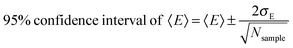 | (25) |
where
σE is the standard deviation of the sampled energy gap data and
Nsample is the number of samples collected (here,
Nsample = 100). The 95% confidence intervals of 〈VIE
EOM-IP-CCSDaq〉 and 〈NVEA
EOM-IP-CCSDaq〉 arising from sampling uncertainty were ≤±0.09 eV in all cases (
Table 3). Recent work demonstrated that the 〈VIE
EOM-IP-CCSDaq〉 is also well-converged with respect to solvated cluster size when 3000 explicit water molecules are included, using the protocol employed here.
12 In the present work, we have assumed that this cluster size is adequate to also converge 〈NVEA
EOM-IP-CCSDaq〉, for the monovalent radical cations that were studied. Finally, consistent with the preliminary observations by Ghosh
et al.,
11 we find that the ΔVIE
aq is converged with respect to basis set with the EOM-IP-CCSD/6-31+G(d) model chemistry. We tested this by evaluating solvent-induced shifts in the vertical gap energy for imidazole embedded in solvent clusters of 32 explicit water molecules, using EOM-IP-CCSD to model the solute and EFPs to model the solvent molecules. Results obtained with the 6-31+G(d) basis set differed from those obtained with 6-311+G(2df,2pd) by only 0.006 ± 0.003 eV (
n = 5), with a maximum discrepancy of 0.011 eV.
Table 3 Aqueous reorganization energies determined under the linear response approximation according to eqn (30)
| |
Aniline |
Methoxybenzene |
DMS |
Imidazole |
Phenol |
| 〈VIEaq〉 |
〈VEAaq〉 |
〈VIEaq〉 |
〈VEAaq〉 |
〈VIEaq〉 |
〈VEAaq〉 |
〈VIEaq〉 |
〈VEAaq〉 |
〈VIEaq〉 |
〈VEAaq〉 |
|
σ
100
2 is the computed variance in the vertical gap energy from a sample of 100 snapshots from EOM-IP-CCSD/6-31+G(d)/EFP computations on solvated clusters consisting of the solute and 3072 water molecules.
λ
LRAIIaq is the computed reorganization energy determined from eqn (30) using 100 snapshots.
σ
500
2 is the computed variance in the vertical gap energy from a sample of 500 snapshots from EOM-IP-CCSD/6-31+G(d)/EFP computations on solvated clusters consisting of the solute and 3072 water molecules.
λ
LRAII,500aq is determined in the same manner as λLRAIIaq, but using 500 snapshots.
σ
expt
2 is determined by Gaussian fit from experimental aqueous PES data.12
λ
LRAII,exptaq is calculated from σexpt2 using eqn (30).
|
|
σ
100
2a |
0.192 |
0.115 |
0.121 |
0.193 |
0.198 |
0.148 |
0.156 |
0.145 |
0.180 |
0.204 |
|
λ
LRAIIaqb |
3.744 |
2.239 |
2.359 |
3.764 |
3.852 |
2.888 |
3.044 |
2.831 |
3.514 |
3.978 |
|
σ
500
2c |
0.180 |
|
0.137 |
|
0.162 |
|
0.164 |
|
0.164 |
|
|
λ
LRAII,500aqd |
3.498 |
2.672 |
3.159 |
3.187 |
3.194 |
|
|
|
σ
expt
2e |
0.186 |
|
|
0.335 |
0.221 |
|
λ
LRAII,exptaqf |
3.620 |
6.517 |
4.312 |
Nonlinear solvent response contribution, ΔΔΔGnon-LRsolv
In order to obtain the complete change in free energy of solvation upon ionization, ΔΔGsolv, the linear solvent response contribution (ΔΔGLRAsolv) is amended with a computed contribution from non-linear solvent response, ΔΔΔGnon-LRsolv (eqn (19)). The ΔΔΔGnon-LRsolv was determined as the difference between the free energy of one-electron oxidation as computed by thermodynamic integration (AIETIaq) and that computed by free energy perturbation (AIEFEPaq), using a classical Hamiltonian in both cases (eqn (24)) (Fig. S5, ESI†). For the neutral molecules tested here, the ΔΔΔGnon-LRsolv contribution ranged from −0.07 eV (methoxybenzene) to −0.14 eV (DMS). Thus the ΔΔΔGnon-LRsolv term is about an order of magnitude smaller than the ΔΔGLRAsolv contribution to the total ΔΔGsolv (Table 2).
Among the five solutes, the largest computed ΔΔΔGnon-LRsolv values are found for the two compounds that exhibit a reversal of sign (− to +) in (non-zero) RESP charges of at least one atom upon ionization: DMS and phenol (Table 2 and Fig. S6, ESI†). The solvent-exposed sulfur atom of DMS was assigned RESP charges of −0.14 and +0.45 in the neutral and oxidized states, respectively. For phenol, the net RESP charges of the para –CH group (in the phenyl ring) are −0.34 and +0.32 in the neutral and oxidized states, respectively. According to these electrostatic charge assignments, the proximate solvent molecule may be expected to undergo a complete reorientation upon ionization, and this is consistent with the conditions expected to lead to nonlinear response of the solvent.67,116 The other studied solutes (imidazole, methoxybenzene, and aniline) do not exhibit this attribute, consistent with the observed slightly lower ΔΔΔGnon-LRsolv values compared to those for DMS and phenol. It is worth noting that natural population analysis (NPA) charges, computed with SMD119/M06-2X120/aug-cc-pVTZ, produce a somewhat different electrostatic distribution than the RESP charges, which were computed in gas phase with M05-2X/aug-cc-pVDZ (Fig. S3 and S6, ESI†). Future work in this area would benefit from further evaluation of the most appropriate choice of electrostatic charge assignments used for the determination of ΔΔΔGnon-LRsolv.
We find larger non-linear solvent response contributions than have been reported previously for other organic solutes. Cheng et al. evaluated differences in AIETIaq and AIEFEPaq for both the one-electron reduction and one-electron oxidation of benzoquinone, finding non-linear response contributions of ≤0.05 eV for this neutral molecule.24 The ΔΔΔGnon-LRsolv found for benzoquinone is smaller than the values found for molecules studied here (Table 2). This is consistent with our interpretation (discussed above) that trends in the ΔΔΔGnon-LRsolv are explainable in terms of the extent of charge localization on the ionized solute: the oxidized radical cation (or reduced radical anion) produced by one-electron oxidation (or reduction) of benzoquinone is expected to exhibit greater charge delocalization than the ionized solutes considered in the present study. Little is otherwise known about the magnitude of non-linear solvent response for the single-electron oxidation/reduction of neutral organic molecules in water. Conducting DFT-MD simulations of the one-electron oxidations of tetrathiafulvalene (TTF) and thianthrene (TH) in the polar aprotic solvent acetonitrile, Vandevondele et al. found parabolic vertical gap energy distributions, suggesting applicability of the LRA. However the resulting half-cell λLRAaq values differed by >0.2 eV for the oxidation of TH versus for the reduction of TH˙+.21 Nonetheless, their approach reasonably reproduced experimental free energy differences for the SET between TH˙+ and TTF and for the SET between TH2+ and TTF˙+.
Finally, for redox pairs such as CO2/CO2˙− that have vertical ionization gaps approaching the band edge of water, the non-linear solvent response component may strongly increase, due to the mixing of vertical electronic states of the solute and the solvent.117 The computational protocol of the present study has not been designed to handle such cases, which would require fully QM simulation of (at least) the solvent molecules immediately proximate to the solute. Such mixed vertical states are not expected to arise for the solutes tested here, all of which have VIEaq and NVEAaq values that differ from the valence band energies of water by ≥1.3 V.
Free energy contributions to Eox from the gas phase and from the solvent: AIErefgas and ΔΔGsolv
The Eox is determined from the adiabatic free energy of one-electron oxidation in solution, AIEaq, by eqn (23). Our computed AIErefaq values can be viewed as originating from three summed free energy components: the contribution from ionization in gas phase (AIErefgas); a contribution arising from linear response of the solvent (ΔΔGLRAsolv); and a non-linear solvent response contribution (ΔΔΔGnon-LRsolv), as shown by eqn (18) and (19). The largest free energy contribution is the AIErefgas, followed by the linear solvent response component, ΔΔGLRAsolv. For the compounds in the test set, the AIErefgas ranges from 7.73 to 8.82 eV. The magnitude of the ΔΔGLRAsolv term lies between −2.01 and −2.73 eV, or roughly one-third the size of the gas phase component, but with opposite sign (Fig. 2). The ΔΔΔGnon-LRsolv term is the smallest contribution, ranging from −0.07 eV to −0.14 eV. These results illustrate that a priori predictions of Eox having “chemical accuracy” (≤0.04 V error) would require the inclusion of all three energy components, computed correctly, for the molecule set considered here.
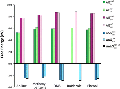 |
| | Fig. 2 Adiabatic free energy of the aqueous one-electron oxidation (AIErefaq) and the disaggregated free energy properties, AIErefgas, ΔΔGLRAsolv, and ΔΔΔGnon-LRsolv, for several organic molecules. AIEexptaq is the aqueous free energy of oxidation as calculated from the experimental oxidation potential (Table 1). AIErefaq is the computed free energy of oxidation determined by eqn (18). AIEexptgas is the reported gas phase experimental adiabatic ionization energy at 0 K (Table 1), and AIErefgas is the gas phase adiabatic ionization energy determined by eqn (6). ΔΔGexptsolv is the difference in free energy of solvation between the oxidized and reduced species as determined from the experimentally available oxidation potential and gas phase adiabatic ionization energy.51 ΔΔGLRAsolv is determined by eqn (17), and ΔΔΔGnon-LRsolv is computed by eqn (24). | |
The total change in free energy of solvation upon oxidation, ΔΔGsolv, is instructive because it indicates the extent to which the solvent influences the free energy of oxidation. The computed ΔΔGsolv ranges from −2.08 (methoxybenzene) to −2.83 eV (imidazole), spanning a range of 0.75 eV for the five compounds considered here. We can make comparisons with experimentally derived ΔΔGexptsolv values based on experimentally available Eox,aq and AIEgas values, as described in Guerard and Arey.51 Computed ΔΔGsolv values are in good agreement with ΔΔGexptsolv values, exhibiting an MUE of 0.19 eV for the four compounds where these quantities can be compared (Table 2 and Fig. 2). Trends in computed ΔΔGsolv are also roughly consistent with experimental values. For example, within the set, methoxybenzene exhibits the smallest ΔΔGexptsolv value (−2.37 eV) and also the smallest computed ΔΔGsolv value (−2.09 eV). Similarly, DMS exhibits the largest ΔΔGsolv value and also the largest ΔΔGexptsolv value. For the compounds considered here, the largest contributor to variability in the ΔΔGsolv is the ΔNVEAaq, followed by ΔVIEaq, with the least variability arising from ΔΔΔGnon-LRsolv. Trends in the ΔΔGsolv therefore can be thought of in terms of the structural features that regulate the underlying quantities ΔVIEaq, ΔNVEAaq, and ΔΔΔGnon-LRsolv, including the extent of charge localization of the oxidized radical cation species and the presence of hydrogen-bond donor groups on both the reduced and oxidized species, as discussed in previous sections.
Performance of predictions for Eox by explicit solvent simulations
Simulated aqueous single electron oxidation potentials from first principles exhibit a mean unsigned error of 0.17 V and a maximum absolute error of 0.28 V with respect to available experimental Eox data for four compounds (Table 1 and Fig. 3). Predictions for aniline and DMS exhibit errors of −0.13 V and −0.15 V respectively. Predictions for methoxybenzene and phenol exhibited larger errors of +0.28 V and +0.26 V, respectively. The explicit solvent method provides slightly better results on average than the implicit solvent model, SMD (Table 1). In particular, the largest error of the explicit solvent model (0.28 V) is considerably smaller than the largest error of the implicit solvent model (0.42 V). In comparing the two models, it is worth remarking that implicit solvent models have been re-developed and re-fitted empirically with thousands of experimental solvation energy data by several independent research groups over several decades. By comparison, the explicit method presented here is a 1st generation ab initio approach that was not fitted using any experimental solvation energy data and likely could be submitted to further improvements in future studies.
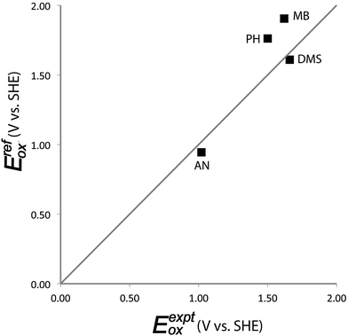 |
| | Fig. 3 Comparison of computed aqueous single-electron oxidation potentials from explicitly solvated simulations versus experimental values. AN = aniline, MB = methoxybenzene, DMS = dimethylsulfide, PH = phenol. | |
For the case of phenol, our method exhibited an error of similar magnitude, but opposite sign, to that of Ghosh et al.,11 who obtained a deviation of −0.28 V from the experimental Eox. The 0.54 V discrepancy in the computed value of Eox between the two studies arises largely from the difference in computed ΔNVEAaq values of the oxidized radical cation of phenol. As discussed above, we infer that this difference is primarily due to the choice of Hamiltonian used to generate the solvated trajectories. Differences in computed Eox values reported by the two studies are (to a lesser extent) also due to our incorporation of an energy contribution from non-linear solvent effects (−0.11 eV for phenol) and our incorporation of highly accurate reference gas phase values (also not included by Ghosh et al.).
Consideration of the disaggregated thermodynamic energy components contained in AIErefaq provides direct insight into the origins of uncertainty in our computational estimates of Eox. The computed change in free energy of solvation upon oxidation, ΔΔGsolv, has much larger error (∼0.20 eV) than the computed free energy of ionization in gas phase, AIErefgas (∼0.04 eV). The errors in ΔΔGsolv are, in turn, largely due to uncertainties in computed ΔVIEaq and ΔNVEAaq values. Improved methods to compute ΔVIEaq and ΔNVEAaq therefore represent the key advance needed to obtain improved predictions of Eox from first principles, for the neutral solutes studied here.
The aqueous reorganization energy
The computed aqueous reorganization energy of the oxidation half-cell reaction can be defined in three different ways, each of which produces different results: (1) by eqn (20) (λrefaq), which closes the thermodynamic cycle between VIErefaq and AIErefaq (Fig. 1) and is not restricted by the linear response approximation;19 (2) by the linear response approximation according to eqn (21) (λLRAaq), which is equivalent to eqn (20) under the LRA; or (3) by the relationship that arises between the variance of the fluctuations in the vertical gap and the reorganization energy15 (here called λLRAIIaq) under the LRA. Each of these different computational interpretations is discussed in turn below, including comparisons to experimental data where available.
The electrochemical definition, eqn (20), is considered here to be the most general and thermodynamically consistent description of the aqueous reorganization energy. Our simulation estimates of λrefaq are in excellent agreement with recently reported experimental data (λexptaq)12 that are available for the two compounds aniline and phenol, exhibiting discrepancies of only 0.10 and 0.01 eV, respectively (Table 1). Experimentally derived λaq values were determined previously by eqn (20) based on experimental VIEaq data from aqueous liquid microjet photoelectron spectroscopy measurements and reported experimental AIEaq data from pulse radiolysis measurements of the oxidation potential.12 Simulated λrefaq values for the five compounds studied here range from 1.95 eV (methoxybenzene) to 2.45 eV (imidazole). These values are about an order of magnitude larger than the gas phase reorganization energies (λrefgas) for these same compounds, which range from 0.16 to 0.31 eV (Table 1), demonstrating that the aqueous solvent is responsible for the dominant contribution to the reorganization.
In order to better understand the physical origins of λrefaq, we separately consider the gas phase reorganization energy (λrefgas) and the shift in the reorganization energy upon moving from gas phase into aqueous solution (Δλrefaq).
| | | λrefaq = λrefgas + Δλrefaq | (26) |
Δ
λrefaq is the dominant term in
eqn (26) (
Table 2). Similar to trends in the magnitude of ΔNVEA
aq discussed above, trends in the Δ
λrefaq appear to have a positive relationship with the extent of charge localization on the ionized solute. DMS and imidazole have the largest magnitudes of both ΔNVEA
aq and Δ
λrefaq, and they both exhibit the greatest extent of charge localization on the ionized solute, according to NPA charges computed with SMD/M06-2X/aug-cc-pVTZ (Fig. S3, ESI
†). This is intuitively consistent with the expectation that the free energy change associated with solvent reorganization is strongly related to the creation or redistribution of localized charge density on the solute as a result of the ionization.
65 The gas phase reorganization energy,
λrefgas, is the free energy gain upon relaxing the structure of the ionized solute from the non-equilibrium (
rred) geometry to its equilibrium (
rox) geometry.
Further insight into contributions to Δλrefaq in terms of computationally or experimentally accessible properties can be gained by consideration of eqn (9), (10), (18), (20) and (26), which can be used to deduce that
| | | λrefaq = λrefgas + ΔVIEaq − ΔΔGsolv | (27) |
As has been shown previously,
12,51 the three terms on the right hand side of
eqn (27) all can be obtained from experimental data, in principle. Using
eqn (17), (19), (26) and (27) to further repartition Δ
λrefaq, we find
| | | Δλrefaq = ½(ΔVIEaq) − ½(ΔNVEAaq) − ΔΔΔGnon-LRsolv | (28) |
Thus, the solvent contribution to the reorganization energy is simply related to the solvent-induced shifts in the vertical energy gaps, ΔVIE
aq and ΔNVEA
aq, and a contribution from non-linear solvent response, ΔΔΔ
Gnon-LRsolv. These three contributing terms have widely differing magnitudes, with the ordering |ΔNVEA
aq| > |ΔVIE
aq| > |ΔΔΔ
Gnon-LRsolv| (
Table 2). For the neutral compounds studied here, both the magnitude and the variability in Δ
λrefaq are regulated largely by the terms ΔNVEA
aq and ΔVIE
aq, which are discussed above and in recent work.
12
A second estimate of the aqueous reorganization energy, λLRAaq, can be obtained from the linear response approximation by way of eqn (21). Inspection of eqn (15)–(22) reveals that λLRAaq differs from λrefaq by the amount
| | | λrefaq − λLRAaq = AIELRAaq − AIErefaq = ½(VIErefgas + NVEArefgas) − AIErefgas − ΔΔΔGnon-LRsolv | (29) |
For the compounds studied here,
λLRAaq differs from
λrefaq by −0.08 eV (methoxybenzene) to −0.24 eV (DMS).
λLRAaq exhibits less agreement with available experimental data (
λexptaq) than does
λrefaq (
Table 1). The gas phase energy difference, ½(VIE
refgas + NVEA
refgas) − AIE
refgas, can be viewed as a gas phase contribution to non-linear response. This term ranges from 0.01 to 0.10 eV for the compounds studied here. This is slightly smaller, on average, than the solution phase contribution, ΔΔΔ
Gnon-LRsolv (
Table 2). However, both the gas phase and solvent non-linear response contributions to the reorganization energy are substantial, lending support to the supposition that non-linear response contributions are appropriate to include in computational estimates of both
λaq and AIE
aq.
In addition to the definitions discussed above, the aqueous reorganization energy can be estimated by a third means, labeled here as λLRAIIaq. According to the linear response approximation, thermally induced fluctuations in the vertical energy gap produce a population distribution that has Gaussian curvature, and the variance of this distribution is assumed independent of the oxidation state.15 The LRA implies that the reorganization energy for the half-cell reaction is the same going either forward or backward, i.e. the energy of deformation from the oxidized system geometry to the reduced system geometry (in the reduced electronic state) is the same as the energy of deformation from the reduced system geometry to the oxidized system geometry (in the oxidized electronic state). This is illustrated in the well-known parabolic diabatic free energy curves that are used in Marcus theory to characterize electron transfer in solution. As a consequence, the aqueous vertical gap energies, Eox(rred) − Ered(rred) and Eox(rox) − Ered(rox), should exhibit Gaussian-shaped ensemble distributions that are of the same width.15,118 According to the LRA, the aqueous reorganization energy thus can be estimated as
| |  | (30) |
where
σ2 is the variance in the thermalized distribution of the aqueous vertical gap energy.
Computed λLRAIIaq values (Table 3) exhibit startling discrepancies from other computed and experimental estimates of the aqueous reorganization energy. For all five neutral organic molecules, λLRAIIaq values are much larger than LRA reorganization energies computed according to the electrochemical cycle (λLRAaq, eqn (5)), exhibiting disagreements of >1 eV in several cases (compare Tables 1 and 3). Additionally, the λLRAIIaq estimates derived from vertical gap energy distributions of the reduced species differ substantially from λLRAIIaq estimates derived from vertical gap energy distributions of the oxidized species, by amounts ranging from 0.47 to 1.50 eV. On visual inspection, the histograms of the vertical gap energies appear non-Gaussian in several cases (Fig. S7, ESI†). Finally, compared to our reference λrefaq values, the λLRAIIaq estimates are unacceptably erroneous (Tables 1 and 3), despite the fact that total (gas phase plus solvent) non-linear response contributions are relatively modest (<0.3 eV; eqn (29)).
We further investigated the quality of the reorganization energy estimates produced by eqn (30). We considered whether 100 snapshots provided sufficient information to adequately converge the distribution variance, σ2. Increasing the number of vertical gap energy snapshots from 100 to 500, taken from the same 25 ps trajectory, led to changes ranging from 0.15 to 0.69 eV in computed λLRAIIaq values (autocorrelation analysis showed that the 500 snapshots were statistically independent). The resulting computed λLRAII,500aq values nonetheless remain substantially inflated compared to other computational estimates of λaq. We also determined an experimental reorganization energy estimate according to eqn (30), based on the width of the first vertical ionization band according to liquid aqueous microjet photoelectron spectroscopy data. The resulting λLRAII,exptaq estimates exceed experimental reorganization energies (λexptaq) obtained by using the electrochemical cycle (eqn (5)) by >1 eV, consistent with the trends in computational estimates of these same quantities (Tables 1 and 3). Thus eqn (30) is inconsistent with other estimates of the reorganization energy for the neutral organic molecules considered here, irrespective of the methodological approach used (computation or experiment). Additionally, the λLRAIIaq estimate (eqn (30)) requires far more sample data to achieve statistical convergence than does the electrochemical λLRAaq estimate (eqn (5)). The observed large discrepancies in these different estimates of λaq suggest that eqn (30) is very sensitive to non-linear solvent response. Regardless of the system studied, we recommend that results from eqn (30) are checked against eqn (5), if possible, when either computational or experimental data are used to estimate the reorganization energy under the linear response approximation. Ideally, measures (e.g., eqn (24)) should additionally be taken to directly quantify the extent of non-linear solvent response.
Conclusions
In the present study, explicitly solvated molecular dynamics simulations were employed to determine aqueous one-electron oxidation potentials (Eox) and aqueous half-cell reorganization energies (λaq) of several neutral organic molecules. Simulated redox properties achieve good agreement with experimental values, exhibiting an MUE of 0.17 V for Eox (4 values) and an MUE of 0.06 eV for λaq (2 values). This ab initio approach uses no parameters fitted to experimental redox or solvation energy data, and nonetheless it is found to be competitive with other existing models to estimate redox properties.
To gain further insight into the aqueous one-electron oxidation process, we disaggregate the aqueous adiabatic free energy of oxidation (AIEaq) into several well-defined thermodynamic sub-properties (eqn (17)–(19)):
| | | AIEaq = AIEgas + ½(ΔVIEaq + ΔNVEAaq) + ΔΔΔGnon-LRsolv | (31) |
This thermodynamic formulation is facilitated by the fact that the accurately computed gas phase (vertical or adiabatic) ionization property data can be subtracted from accurate experimental aqueous ionization data, thereby isolating the influence of the solvent on the ionization process. For the neutral organic molecules studied here, AIE
aq is dominated by the gas phase component (AIE
gas; 7.73 to 8.82 eV), followed by the linear solvent response component (½ΔVIE
aq + ½ΔNVEA
aq; −2.01 to −2.73 eV), with a small contribution from the non-linear solvent response component (ΔΔΔ
Gnon-LRsolv; −0.07 to −0.14 eV). An important advantage of the approach is that each of these additive sub-properties can be studied in isolation and can be computed separately. Comparisons with available experimental data confirm that our simulations produce accurate results for the properties AIE
gas, ΔVIE
aq, and ΔΔ
Gsolv. Based on additional analysis of simulated solute–solvent interactions, trends in the solvent sub-properties ΔVIE
aq, ΔNVEA
aq, and ΔΔΔ
Gnon-LRsolv appear to be explainable in terms of the structural features of the solute, such as presence of hydrogen-bond donor groups on the solute and the extent of charge localization on the oxidized radical cation species. Such associations may inform future development of more empirical models to estimate redox properties based on chemical structure.
The aqueous reorganization energy, λaq, can be similarly disaggregated into thermodynamic sub-properties (eqn (26) and (28)):
| | | λaq = λgas + ½(ΔVIEaq − ΔNVEAaq) − ΔΔΔGnon-LRsolv | (32) |
The magnitude of
λaq ranges from 1.95 to 2.45 eV for the neutral organic compounds studied here, according to computational estimates. The
λaq is dominated by the solvent-induced shift in negative vertical electron affinity, ½ΔNVEA
aq, with smaller (< 0.5 eV) contributions from ½ΔVIE
aq,
λgas, and ΔΔΔ
Gnon-LRsolv. For these neutral solutes, the aqueous reorganization energy alternatively can be estimated through the linear response approximation, either by using the thermodynamic cycle given by
eqn (22) or by simply neglecting the ΔΔΔ
Gnon-LRsolv term in
eqn (32). Neglect of the ΔΔΔ
Gnon-LRsolv term eliminates the costly thermodynamic integration procedure needed to evaluate this term. Finally, it is worth noting that we have considered only rigid solutes in the present study. For flexible solutes having more pronounced internal rotations or large bending modes, determination of the reorganization energy may require appropriately weighted sampling of multiple stable conformers, and this may increase the computational cost of the simulation protocol.
The aqueous reorganization energy is often estimated from the variance of the fluctuation distributions of the aqueous vertical energy gap quantities, by way of eqn (30) (λLRAIIaq). However we find that the λLRAIIaq disagrees with more thermodynamically consistent definitions of the aqueous reorganization energy (eqn (20), (27) and (32)), regardless of whether computational or experimental data are used. The λLRAIIaq has the additional disadvantage that it converges much more slowly with respect to sampling than the other definitions of λaq considered here. For these reasons, we recommend considerable caution when using the fluctuation distributions of the aqueous vertical gap energies to estimate the reorganization energy.
The principal source of uncertainty in computational Eox and λaq predictions is the linear solvent response component. The linear solvent response contribution is expressed as the simple average of the solvent-induced shifts in the two vertical energy gaps, ½(ΔVIEaq + ΔNVEAaq). Thus, our ability to simulate accurate redox potentials is limited primarily by our ability to compute these two vertical properties accurately. Efforts to advance computational methodologies of Eox and λaq should focus on improving the simulation descriptions of ΔVIEaq and ΔNVEAaq. Among the thermodynamic properties investigated here, the ΔNVEAaq remains perhaps the most difficult to simulate. Future efforts should be focused on improved Hamiltonians for the molecular dynamics trajectories that are used for solvated vertical energy gap computations, as well as improved model chemistries for the solvated vertical gap energies themselves. Appropriate methods must be chosen for the simulation of radical structures121 as well as their electronic interaction with aqueous solvent.122,123 It remains unclear whether EFPs fully capture the important solute–solvent interactions relevant to the oxidation process, and useful future testing could include the extension of the QM region to envelope the first solvation shell. Recent advances in fragment quantum mechanical models suggest that improved electronic descriptions of extended systems, at decreased computational cost, may soon be within reach.124–126
Acknowledgements
J.J.G. was supported by U.S. N.S.F. I.R.F.P. award 0852999, and this work was also supported by Swiss N.S.F. ProDoc TM Grant PDFMP2-123028. Computational simulations were conducted partly at the Swiss National Supercomputing Center (CSCS) and at EPFL centralized HPC facilities. The authors would also like to thank Kristopher McNeill, Silvio Canonica, and Ivano Tavernelli for valuable discussions.
Notes and references
- Y. Paukku and G. Hill, J. Phys. Chem. A, 2011, 115, 4804–4810 CrossRef CAS PubMed.
- S. Canonica, B. Hellrung and J. Wirz, J. Phys. Chem. A, 2000, 104, 1226–1232 CrossRef CAS.
- W. A. Arnold, Environ. Sci.: Processes Impacts, 2014, 16, 832–838 CAS.
- D. J. Jacob, Atmos. Environ., 2000, 34, 2131–2159 CrossRef CAS.
- B. Ervens, B. J. Turpin and R. J. Weber, Atmos. Chem. Phys., 2011, 11, 11069–11102 CrossRef CAS.
- P. Wardman, J. Phys. Chem. Ref. Data, 1989, 18, 1637–1755 CrossRef CAS PubMed.
- S. C. L. Kamerlin, M. Haranczyk and A. Warshel, J. Phys. Chem. B, 2009, 113, 1253–1272 CrossRef CAS PubMed.
- B. Winter and M. Faubel, Chem. Rev., 2006, 106, 1176–1211 CrossRef CAS PubMed.
- B. Jagoda-Cwiklik, P. Slavíček, L. Cwiklik, D. Nolting, B. Winter and P. Jungwirth, J. Phys. Chem. A, 2008, 112, 3499–3505 CrossRef CAS PubMed.
- F. Paesani and G. A. Voth, J. Phys. Chem. B, 2009, 113, 5702–5719 CrossRef CAS PubMed.
- D. Ghosh, A. Roy, R. Seidel, B. Winter, S. E. Bradforth and A. I. Krylov, J. Phys. Chem. B, 2012, 116, 7269–7280 CrossRef CAS PubMed.
- P. R. Tentscher, R. Seidel, B. Winter, J. J. Guerard and J. S. Arey, J. Phys. Chem. B, 2015, 199, 238–256 CrossRef PubMed.
- B. Jagoda-Cwiklik, P. Slavíček, D. Nolting, B. Winter and P. Jungwirth, J. Phys. Chem. B, 2008, 112, 7355–7358 CrossRef CAS PubMed.
- P. Slavíček, B. Winter, M. Faubel, S. E. Bradforth and P. Jungwirth, J. Am. Chem. Soc., 2009, 131, 6460–6467 CrossRef PubMed.
- J. Blumberger and M. Sprik, Lect. Notes Phys., 2006, 704, 481–506 CAS.
- A. Warshel, J. Phys. Chem., 1982, 86, 2218–2224 CrossRef CAS.
- G. King and A. Warshel, J. Chem. Phys., 1990, 93, 8682–8692 CrossRef CAS PubMed.
- J. K. Hwang and A. Warshel, J. Am. Chem. Soc., 1987, 109, 715–720 CrossRef CAS.
- R. Seidel, M. Faubel, B. Winter and J. Blumberger, J. Am. Chem. Soc., 2009, 131, 16127–16137 CrossRef CAS PubMed.
- M. Sulpizi and M. Sprik, J. Phys.: Condens. Matter, 2010, 22, 284116 CrossRef PubMed.
- J. Vandevondele, R. Lynden-Bell, E. J. Meijer and M. Sprik, J. Phys. Chem. B, 2006, 110, 3614–3623 CrossRef CAS PubMed.
- J. Blumberger, Y. Tateyama and M. Sprik, Comput. Phys. Commun., 2005, 169, 256–261 CrossRef CAS PubMed.
- J. Vandevondele, R. Ayala, M. Sulpizi and M. Sprik, J. Electroanal. Chem., 2007, 607, 113–120 CrossRef CAS PubMed.
- J. Cheng, M. Sulpizi and M. Sprik, J. Chem. Phys., 2009, 131, 154504 CrossRef PubMed.
- F. Costanzo, M. Sulpizi, R. G. Della Valle and M. Sprik, J. Chem. Phys., 2011, 134, 244508 CrossRef PubMed.
- D. Sinha, S. Mukhopadhyay and D. Mukherjee, Chem. Phys. Lett., 1986, 129, 369–374 CrossRef CAS.
- S. Pal, M. Rittby, R. J. Bartlett, D. Sinha and D. Mukherjee, Chem. Phys. Lett., 1987, 137, 273–278 CrossRef CAS.
- J. F. Stanton and J. Gauss, J. Chem. Phys., 1994, 101, 8938–8944 CrossRef CAS PubMed.
- P. A. Pieniazek, S. A. Arnstein, S. E. Bradforth, A. I. Krylov and C. D. Sherrill, J. Chem. Phys., 2007, 127, 164110 CrossRef PubMed.
- A. I. Krylov, Annu. Rev. Phys. Chem., 2008, 59, 433–462 CrossRef CAS PubMed.
- P. A. Pieniazek, S. E. Bradforth and A. I. Krylov, J. Chem. Phys., 2008, 129, 074104 CrossRef PubMed.
- L. V. Slipchenko, J. Phys. Chem. A, 2010, 114, 8824–8830 CrossRef CAS PubMed.
- D. Kosenkov and L. V. Slipchenko, J. Phys. Chem. A, 2011, 115, 392–401 CrossRef CAS PubMed.
- B. T. Psciuk, R. L. Lord, B. H. Munk and H. B. Schlegel, J. Chem. Theory Comput., 2012, 8, 5107–5123 CrossRef CAS.
- K. M. Solntsev, D. Ghosh, A. Amador, M. Josowicz and A. I. Krylov, J. Phys. Chem. Lett., 2011, 2, 2593–2597 CrossRef CAS.
- T. Tugsuz, J. Phys. Chem. B, 2010, 114, 17092–17101 CrossRef CAS PubMed.
- J. L. Hodgson, M. Namazian, S. E. Bottle and M. L. Coote, J. Phys. Chem. A, 2007, 111, 13595–13605 CrossRef CAS PubMed.
- M. Namazian and M. L. Coote, J. Phys. Chem. A, 2007, 111, 7227–7232 CrossRef CAS PubMed.
- M. Namazian, C. Y. Lin and M. L. Coote, J. Chem. Theory Comput., 2010, 6, 2721–2725 CrossRef CAS.
- M. Namazian and H. A. Almodarresieh, THEOCHEM, 2004, 686, 97–102 CrossRef CAS PubMed.
- M. Namazian, H. R. Zare and M. L. Coote, Biophys. Chem., 2008, 132, 64–68 CrossRef CAS PubMed.
- M. Namazian, H. A. Almodarresieh, M. R. Noorbala and H. R. Zare, Chem. Phys. Lett., 2004, 396, 424–428 CrossRef CAS PubMed.
- M. Namazian, S. Siahrostami and M. L. Coote, J. Fluorine Chem., 2008, 129, 222–225 CrossRef CAS PubMed.
- R. I. Zubatyuk, L. Gorb, O. V. Shishkin, M. Qasim and J. Leszczynski, J. Comput. Chem., 2010, 31, 144–150 CrossRef CAS PubMed.
- A. Lewis, J. A. Bumpus, D. G. Truhlar and C. J. Cramer, J. Chem. Educ., 2004, 81, 596–604 CrossRef CAS.
- M. Shamsipur, K. Alizadeh and S. Arshadi, THEOCHEM, 2006, 758, 71–74 CrossRef CAS PubMed.
- R. S. Assary, L. A. Curtiss, P. C. Redfern, Z. Zhang and K. Amine, J. Phys. Chem. C, 2011, 115, 12216–12223 CAS.
- M. B. Camarada, P. Jaque, F. R. Díaz and M. A. del Valle, J. Polym. Sci., Part B: Polym. Phys., 2011, 49, 1723–1733 CrossRef CAS PubMed.
- J. P. Blinco, J. L. Hodgson, B. J. Morrow, J. R. Walker, G. D. Will, M. L. Coote and S. E. Bottle, J. Org. Chem., 2008, 73, 6763–6771 CrossRef CAS PubMed.
- C. Y. Lin, M. L. Coote, A. Gennaro and K. Matyjaszewski, J. Am. Chem. Soc., 2008, 130, 12762–12774 CrossRef CAS PubMed.
- J. J. Guerard and J. S. Arey, J. Chem. Theory Comput., 2013, 9, 5046–5058 CrossRef CAS.
- A. V. Marenich, J. Ho, M. L. Coote, C. J. Cramer and D. G. Truhlar, Phys. Chem. Chem. Phys., 2014, 16, 15068–15106 RSC.
- A. Warshel, J. Phys. Chem., 1979, 83, 1640–1652 CrossRef CAS.
- R. A. Kuharski, J. S. Bader, D. Chandler, M. Sprik, M. L. Klein and R. W. Impey, J. Chem. Phys., 1988, 89, 3248–3257 CrossRef CAS PubMed.
- J. Blumberger, Phys. Chem. Chem. Phys., 2008, 10, 5651–5667 RSC.
- J. Blumberger and G. Lamoureux, Mol. Phys., 2008, 106, 1597–1611 CrossRef CAS PubMed.
- J. Blumberger and M. Sprik, Theor. Chem. Acc., 2005, 115, 113–126 CrossRef PubMed.
- J. Blumberger, I. Tavernelli, M. L. Klein and M. Sprik, J. Chem. Phys., 2006, 124, 064507 CrossRef PubMed.
- M. Sulpizi and M. Sprik, Phys. Chem. Chem. Phys., 2008, 10, 5238 RSC.
- J. Moens, R. Seidel, P. Geerlings, M. Faubel, B. Winter and J. Blumberger, J. Phys. Chem. B, 2010, 114, 9173–9182 CrossRef CAS PubMed.
- J. Moens, P. Jaque, F. De Proft and P. Geerlings, J. Phys. Chem. A, 2008, 112, 6023–6031 CrossRef CAS PubMed.
- R. A. Marcus, J. Chem. Phys., 1957, 26, 867–871 CrossRef CAS PubMed.
- R. A. Marcus, J. Chem. Phys., 1957, 26, 872–877 CrossRef CAS PubMed.
- R. A. Marcus, J. Phys. Chem., 1963, 67, 853–857 CrossRef CAS.
- R. A. Marcus, J. Chem. Phys., 1956, 24, 966–978 CrossRef CAS PubMed.
- R. A. Marcus, Discuss. Faraday Soc., 1960, 29, 21 RSC.
- A. Milischuk and D. V. Matyushov, J. Phys. Chem. A, 2002, 106, 2146–2157 CrossRef CAS.
- A. Milischuk and D. V. Matyushov, J. Chem. Phys., 2003, 118, 1859–1862 CrossRef CAS PubMed.
- D. V. Matyushov and G. A. Voth, J. Chem. Phys., 2000, 113, 5413 CrossRef CAS PubMed.
- J. Åqvist and T. Hansson, J. Phys. Chem., 1996, 100, 9512–9521 CrossRef.
- R. Ayala and M. Sprik, J. Phys. Chem. B, 2008, 112, 257–269 CrossRef CAS PubMed.
-
P. J. Mohr, B. N. Taylor and D. B. Newell, “The 2010 CODATA recommended values of physical constants” Web version 6.1, 2011, (http://physics.nist.gov/constants, accessed March 19, 2013) Search PubMed.
- D. G. Truhlar, C. J. Cramer, A. Lewis and J. A. Bumpus, J. Chem. Educ., 2007, 84, 934 CrossRef.
- J. E. Bartmess, J. Phys. Chem., 1994, 98, 6420–6424 CrossRef CAS.
- J. J. Warren, T. A. Tronic and J. M. Mayer, Chem. Rev., 2010, 110, 6961–7001 CrossRef CAS PubMed.
- T. Schwabe and S. Grimme, Phys. Chem. Chem. Phys., 2007, 9, 3397–3406 RSC.
- S. Grimme, J. Chem. Phys., 2006, 124, 034108 CrossRef PubMed.
- F. Weigend and R. Ahlrichs, Phys. Chem. Chem. Phys., 2005, 7, 3297–3305 RSC.
-
M. J. Frisch, G. W. Trucks, H. B. Schlegel, G. E. Scuseria, M. A. Robb, J. R. Cheeseman, G. Scalmani, V. Barone, B. Mennucci, G. A. Petersson, H. Nakatsuji, M. Caricato, X. Li, H. P. Hratchian, A. F. Izmaylov, J. Bloino, G. Zheng, J. L. Sonnenberg, M. Hada, M. Ehara, K. Toyota, R. Fukuda, J. Hasegawa, M. Ishida, T. Nakajima, Y. Honda, O. Kitao, H. Nakai, T. Vreven, J. A. Montgomery Jr., J. E. Peralta, F. Ogliaro, M. Bearpark, J. J. Heyd, E. Brothers, K. N. Kudin, V. N. Staroverov, R. Kobayashi, J. Normand, K. Raghavachari, A. Rendell, J. C. Burant, S. S. Iyengar, J. Tomasi, M. Cossi, N. Rega, J. M. Millam, M. Klene, J. E. Knox, J. B. Cross, V. Bakken, C. Adamo, J. Jaramillo, R. Gomperts, R. E. Stratmann, O. Yazyev, A. J. Austin, R. Cammi, C. Pomelli, J. W. Ochterski, R. L. Martin, K. Morokuma, V. G. Zakrzewski, G. A. Voth, P. Salvador, J. J. Dannenberg, S. Dapprich, A. D. Daniels, Ö. Farkas, J. B. Foresman, J. V. Ortiz, J. V. Cioslowski and D. J. Fox, Gaussian 09, Gaussian, Inc., Wallingford, CT, 2009 Search PubMed.
- V. Barone, J. Chem. Phys., 2005, 122, 014108 CrossRef PubMed.
- C. I. Bayly, P. Cieplak, W. D. Cornell and P. A. Kollman, J. Phys. Chem., 1993, 97, 10269–10280 CrossRef CAS.
- Y. Zhao, N. E. Schultz and D. G. Truhlar, J. Chem. Theory Comput., 2006, 2, 364–382 CrossRef.
- R. A. Kendall, T. H. Dunning and R. J. Harrison, J. Chem. Phys., 1992, 96, 6796–6806 CrossRef CAS PubMed.
-
D. A. Case, T. A. Darden, T. E. Cheatham, C. L. Simmerling, J. Wang, R. E. Duke, R. Luo, R. C. Walker, W. Zhang, K. M. Merz, B. Roberts, B. Wang, S. Hayik, A. Roitberg, G. Seabra, I. Kolossváry, K. F. Wong, F. Paesani, J. Vanicek, J. Liu, X. Wu, S. R. Brozell, T. Steinbrecher, H. Gohlke, Q. Cai, X. Ye, M.-J. Hsieh, G. Cui, D. R. Roe, D. H. Mathews, M. G. Seetin, C. Sagui, V. Babin, T. Luchko, S. Gusarov, A. Kovalenko and P. A. Kollman, AMBER 10, University of California, San Francisco, 2010 Search PubMed.
- J. Wang, R. M. Wolf, J. W. Caldwell, P. A. Kollman and D. A. Case, J. Comput. Chem., 2004, 25, 1157–1174 CrossRef CAS PubMed.
- J. W. Caldwell and P. A. Kollman, J. Phys. Chem., 1995, 99, 6208–6219 CrossRef CAS.
- J.-P. Ryckaert, G. Ciccotti and H. J. C. Berendsen, J. Comput. Phys., 1977, 23, 327–341 CrossRef CAS.
- T. Laino, F. Mohamed, A. Laio and M. Parrinello, J. Chem. Theory Comput., 2006, 2, 1370–1378 CrossRef CAS.
- T. Laino, F. Mohamed, A. Laio and M. Parrinello, J. Chem. Theory Comput., 2005, 1, 1176–1184 CrossRef CAS.
-
The CP2K Developers Group, cp2k.org, 2012 Search PubMed.
- S. Grimme, J. Comput. Chem., 2006, 27, 1787–1799 CrossRef CAS PubMed.
- M. Krack, Theor. Chem. Acc., 2005, 114, 145–152 CrossRef CAS.
- G. Lippert, J. Hutter and M. Parrinello, Theor. Chem. Acc., 1999, 103, 124–140 CrossRef CAS.
- J. Vandevondele, M. Krack, F. Mohamed, M. Parrinello, T. Chassaing and J. Hutter, Comput. Phys. Commun., 2005, 167, 103–128 CrossRef CAS PubMed.
- J. Vandevondele and J. Hutter, J. Chem. Phys., 2003, 118, 4365 CrossRef CAS PubMed.
- J. Vandevondele and M. Sprik, Phys. Chem. Chem. Phys., 2005, 7, 1363–1367 RSC.
- T. Laino and J. Hutter, J. Chem. Phys., 2008, 129, 074102 CrossRef PubMed.
- P. P. Ewald, Ann. Phys., 1921, 369, 253–287 CrossRef PubMed.
- W. Hoover, Phys. Rev. A: At., Mol., Opt. Phys., 1985, 31, 1695–1697 CrossRef.
- W. J. Hehre, J. Chem. Phys., 1972, 56, 2257–2261 CrossRef CAS PubMed.
- P. C. Hariharan and J. A. Pople, Theor. Chem. Acc., 1973, 28, 213–222 CrossRef CAS.
- M. M. Francl, J. Chem. Phys., 1982, 77, 3654–3665 CrossRef CAS PubMed.
- T. Clark, J. Chandrasekhar, G. N. W. Spitznagel and P. V. R. Schleyer, J. Comput. Chem., 1983, 4, 294–301 CrossRef CAS PubMed.
- M. S. Gordon, M. A Freitag, P. Bandyopadhyay, J. H. Jensen, V. Kairys and W. J. Stevens, J. Phys. Chem. A, 2001, 105, 293–307 CrossRef CAS.
- Y. Shao, L. F. Molnar, Y. Jung, J. R. Kussmann, C. Ochsenfeld, S. T. Brown, A. T. B. Gilbert, L. V. Slipchenko, S. V. Levchenko, D. P. O Neill, R. A. DiStasio Jr, R. C. Lochan, T. Wang, G. J. O. Beran, N. A. Besley, J. M. Herbert, C. Yeh Lin, T. Van Voorhis, S. Hung Chien, A. Sodt, R. P. Steele, V. A. Rassolov, P. E. Maslen, P. P. Korambath, R. D. Adamson, B. Austin, J. Baker, E. F. C. Byrd, H. Dachsel, R. J. Doerksen, A. Dreuw, B. D. Dunietz, A. D. Dutoi, T. R. Furlani, S. R. Gwaltney, A. Heyden, S. Hirata, C.-P. Hsu, G. Kedziora, R. Z. Khalliulin, P. Klunzinger, A. M. Lee, M. S. Lee, W. Liang, I. Lotan, N. Nair, B. Peters, E. I. Proynov, P. A. Pieniazek, Y. Min Rhee, J. Ritchie, E. Rosta, C. David Sherrill, A. C. Simmonett, J. E. Subotnik, H. Lee Woodcock III, W. Zhang, A. T. Bell, A. K. Chakraborty, D. M. Chipman, F. J. Keil, A. Warshel, W. J. Hehre, H. F. Schaefer III, J. Kong, A. I. Krylov, P. M. W. Gill and M. Head-Gordon, Phys. Chem. Chem. Phys., 2006, 8, 3172–3191 RSC.
- I. Adamovic and M. S. Gordon, Mol. Phys., 2005, 103, 379–387 CrossRef CAS PubMed.
- L. Kleinman, Phys. Rev. B: Condens. Matter Mater. Phys., 1981, 24, 7412–7414 CrossRef CAS.
- D. Asthagiri, L. R. Pratt and H. S. Ashbaugh, J. Chem. Phys., 2003, 119, 2702–2708 CrossRef CAS PubMed.
- P. Hunt and M. Sprik, ChemPhysChem, 2005, 6, 1805–1808 CrossRef CAS PubMed.
- C. Adriaanse, M. Sulpizi, J. Vandevondele and M. Sprik, J. Am. Chem. Soc., 2009, 131, 6046–6047 CrossRef CAS PubMed.
- M. Bietti, E. Baciocchi and S. Steenken, J. Phys. Chem. A, 1998, 102, 7337–7342 CrossRef CAS.
- M. Jonsson, J. Lind, T. E. Eriksen and G. Merényi, J. Am. Chem. Soc., 1994, 116, 1423–1427 CrossRef CAS.
- M. Jonsson, J. Lind, T. Reitberger, T. E. Eriksen and G. Merényi, J. Phys. Chem., 1993, 97, 11278–11282 CrossRef CAS.
- G. Merényi, J. Lind and L. Engman, J. Phys. Chem., 1996, 100, 8875–8881 CrossRef.
-
R. E. Walpole and R. H. Myers, Probability and Statistics for Engineers and Scientists, Pearson, New York, 4th edn, 1989 Search PubMed.
- D. V. Matyushov, J. Chem. Phys., 2004, 120, 1375 CrossRef CAS PubMed.
- C. Adriaanse, J. Cheng, V. Chau, M. Sulpizi, J. Vandevondele and M. Sprik, J. Phys. Chem. Lett., 2012, 3, 3411–3415 CrossRef CAS.
- M. Tachiya, J. Phys. Chem., 1993, 97, 5911–5916 CrossRef CAS.
- A. V. Marenich, C. J. Cramer and D. G. Truhlar, J. Phys. Chem. B, 2009, 113, 6378–6396 CrossRef CAS PubMed.
- Y. Zhao and D. G. Truhlar, Theor. Chem. Acc., 2008, 120, 215–241 CrossRef CAS.
- P. R. Tentscher and J. S. Arey, J. Chem. Theory Comput., 2012, 8, 2165–2179 CrossRef CAS.
- P. R. Tentscher and J. S. Arey, J. Chem. Theory Comput., 2013, 9, 1568–1579 CrossRef CAS.
- P. R. Tentscher and J. S. Arey, J. Phys. Chem. A, 2013, 117, 12560–12568 CrossRef CAS PubMed.
- S. Li, W. Li and J. Ma, Acc. Chem. Res., 2014, 47, 2712–2720 CrossRef CAS PubMed.
- B. Wang, K. R. Yang, X. Xu, M. Isegawa, H. R. Leverentz and D. G. Truhlar, Acc. Chem. Res., 2014, 47, 2731–2738 CrossRef CAS PubMed.
- S. R. Pruitt, C. Bertoni, K. R. Brorsen and M. S. Gordon, Acc. Chem. Res., 2014, 47, 2786–2794 CrossRef CAS PubMed.
Footnote |
| † Electronic supplementary information (ESI) available: Text pertaining to computational methods and figures pertaining to convergence of VIE quantities during the molecular dynamics simulation, as well as autocorrelation and normality plots of computed vertical gap quantities. Also included are plots of diabatic free energy curves, thermodynamic integration results, depictions of RESP and NPA charges on each atom for each molecule within the test set, and an example input file/keyword selection for the QM/MM molecular dynamics trajectories produced in CP2K. See DOI: 10.1039/c4cp04760e |
|
| This journal is © the Owner Societies 2015 |
Click here to see how this site uses Cookies. View our privacy policy here. 
 Open Access Article
 This Open Access Article is licensed under a Creative Commons Attribution-Non Commercial 3.0 Unported Licence


