Dynamics of correlated forces in lattice model of granular solids near jamming

Abstract

We investigate the dynamics of a simple lattice model of granular solids near jamming, using a Monte Carlo simulation that samples the ensemble of force networks consistent with a given average stress and distance from the isostatic point J. The Hamiltonian is simply the number of nearest-neighbor pairs that bear no force (“zero bonds”); as the simulation “temperature” decreases, the system is depleted of force-bearing contacts. We find that as point J approaches, various measures of the dynamics become extremely slow, with power-law divergences of characteristic times. We also observe dynamic heterogeneity, with a growing length scale defined by the spatial correlations of the persistence function for zero bonds. The model appears to approach point J at a finite temperature, at which various timescales diverge without an obvious corresponding divergence in the correlation length of some static order parameter, suggesting that this lattice model exhibits a hallmark of a dynamical glass transition.

---

1 Introduction

The nature of the glass transition has been the object of enduring interest, described by some as the most interesting unsolved problem in condensed matter physics.^1–6 Over the past decade, intense and sustained efforts have been focused on a closely related problem, the dynamical behavior of granular materials. Both glassy and granular materials are amorphous systems of particles in which the dynamics changes dramatically, in what may be described as a transition between fluid-like and solid-like states, but without the appearance of any obvious long-range order.

It has been argued that the glass transition in molecular fluids, most typically accessed by temperature (but affected by pressure) is one manifestation of a more general jamming transition, which may be approached either by cooling, applying stress, or increasing the volume fraction of particles.⁷ This argument serves to justify a focus on the hard-sphere jamming transition at zero temperature and stress (denoted by point J), as a simpler proxy for investigating the glass transition more generally. The relative simplicity of simulating hard or nearly-hard colloidal particles, and of exploring such experimental systems with confocal microscopy and rheology, has made this avenue of research very fruitful.^8–11

The main feature of granular materials is that they can support stress like solids, or flow like liquids, depending on conditions. Jamming is the point at which a fluid granular system becomes solid-like. The jammed state has no static long-range order in the positions of particles. At point J, a granular system is isostatic, meaning that there are just enough forces acting between particles to satisfy force balance on every particle. Well into the jammed state, there are many more forces acting between particles than the minimum number necessary for static equilibrium, so that there is a large degeneracy in the arrangement of forces consistent with static equilibrium.⁷ Static properties of jamming systems in both d = 2 and d = 3 dimensions, such as pressure, bulk and shear modulus, were extensively studied by O'Hern et al.,^12,13 who demonstrated that these quantities scale as power laws with excess volume fraction near point J.

Granular materials also display signatures of a dynamical transition as point J is approached. A fascinating aspect of the dynamical slowing in these materials is that it occurs without an obvious accompanying static order parameter. Thus some features of the jamming transition appear to be consistent with a conventional second-order phase transition (power law divergences of various static quantities), yet an accompanying static correlation length has not been identified.

A key feature of glassy dynamics is heterogeneity: slowly and rapidly evolving regions coexist, with a characteristic size significantly larger than the molecular scale. Dynamical heterogeneity has been observed both in experiments¹⁴ and in numerical simulations.^15,16 Dynamical heterogeneity is typically accompanied by observation of nonexponential relaxation of macroscopic quantities, often reasonably fit by stretched exponentials. Despite these observations, no clear consensus exists for the generic origin of dynamical heterogeneity, or for the expected growth of the corresponding correlation length as the glass or jamming transition is approached.

Convenient and appealing as hard- and nearly-hard sphere models are to simulate and study, lattice models are simpler still. Snoeijer et al.¹⁷ and Unger et al.¹⁸ exploited contact networks by investigating on the restricted ensemble of force configurations for a fixed packing configuration. Tighe et al.¹⁹ introduced a lattice model of a jammed system designed to explore the degeneracy of force networks well above the isostatic point, bearing some large average stress. In our previous work,²⁰ we adapted this lattice model to study the approach to jamming from the solid side of the transition.

The resulting model may be regarded as exploring an ensemble of slightly rough, nearly hard particles forced into a lattice, in which only elastic contacts bear (repulsive) force. Point J is approached by depleting the system of force-bearing bonds, which may be thought of as increasing the roughness of the particles. The force configurations as point J is approached showed no long-range correlations; however, perturbations of the force network subject to the constraint that no missing contacts be newly engaged were observed to exhibit a diverging length scale in the isostatic limit.²⁰

More generally, our model may be regarded as a new form of facilitated spin model,^21,22 in which the requirement that bonds cannot bear negative forces serves to restrict the possible local rearrangements. On physical grounds, we expect the number of excess degrees of freedom to vanish as point J is approached. From our simulations, it appears that this condition corresponds to a finite value of the control parameter (i.e., finite “temperature”). Thus our model is of potential interest as a proper Hamiltonian lattice model with a dynamical transition at finite control parameter.

In the present paper, we focus on the dynamical properties of our lattice model of jamming. In particular, we examine the autocorrelation function of bond forces, the persistence of the zero or nonzero state of bonds, and the corresponding spatial correlations of the persistence of bonds, in the manner now commonly applied in other studies of glassy systems.^15,16 This paper is arranged as follows. Section 2, briefly describes our lattice model of jamming, first introduced in ref. 19. In Section 3 and Section 4, dynamical analysis is carried out for the bond force network and the dual structure of “force tiles”, respectively. A discussion and conclusions section follows.

2 Model

In our lattice model of jamming,^19,20 a jammed granular system in d = 2 dimensions is modeled as a regular hexagonal packing of hard disks of equal size, in which each particle has six neighboring particles.

All forces in the model are central, acting along the vector between the centers of neighboring particles. Since attractive interactions are negligible in granular materials, the forces are required to be repulsive. For convenience in simulation, the magnitude of forces are quantized, in units of some arbitrary smallest force. A force magnitude can be zero or any positive integer.

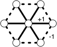
Tighe et al. introduced the wheel move as a way to explore the degeneracy of jammed force networks well above point J.¹⁹ The wheel move can be thought of physically for a system of nearly-hard particles as a slight swelling (or shrinking) of the central particle, with a corresponding slight shrinking (or swelling) of the surrounding particles in the direction of the affected contact with the next neighbor around the ring. This slight change in the shapes of the particles alters the force borne by all of the involved contacts. This collective change in forces is the wheel move shown in Fig. 1. The “amplitude” of a wheel move is the magnitude of the force change on each bond in a wheel move.

Fig. 1 Wheel move. Positive (negative) force changes shown as solid (dashed) lines.

Any wheel move performed on a state in static equilibrium, always produces another state in static equilibrium.¹⁹ Note also that the set of wheel moves is linearly independent, i.e., a given wheel move cannot be written as a finite linear superposition of other wheel moves. (If identical wheel moves are performed on every site in the system, the forces are unchanged, but this is the only degeneracy.) In the hexagonal lattice with its three bonds per particle, there is one more bond per particle than the two bonds necessary in d = 2 dimensions to maintain static equilibrium on all particles.

Hence there are as many independent wheel moves as there are excess degrees of freedom in the force network, so the set of wheel moves is ergodic—sufficient to explore the ensemble of force networks at static equilibrium with a fixed average stress. Invoking the physical interpretation described above, we may say that this ensemble of force networks corresponds to an ensemble of slightly rough particles packed into a hexagonal lattice at fixed average stress.

Ref. 19 reports the results of unbiased Monte Carlo simulations using randomly chosen wheel moves, undertaken to explore the degeneracy in force networks.¹⁹ By introducing a bias towards states with more bonds bearing zero force, we can control the distance from the isostatic limit and investigate the properties of a jammed system as it approaches the jamming transition.

We penalize moves that decrease the number of zero bonds by defining the energy of a state E to be equal to the number of zero bonds B. A conventional Monte Carlo simulation is carried on at some fictitious inverse temperature β.

For each Monte Carlo step, a wheel move with unit amplitude is proposed on a random lattice site. The move is accepted or rejected according to the Metropolis acceptance rule. Moves that would result in a bond bearing a negative (attractive) force are always rejected. This requirement (effectively infinite energy for negative forces) increasingly constrains the simulation as the isostatic point is approached, leading to increasingly slow dynamics.

Large values of β will strongly bias the system towards states with large numbers of zero bonds. By adjusting β, we can approach the jamming transition in a controlled fashion. Since the wheel move preserves force balance of the system, the ensemble of force networks has fixed average stress. For simplicity, we begin our simulations with a lattice of constant force magnitude, which we choose to be large enough so that a wheel move of integer amplitude is a relatively small change to the force network (in this work we take f₀ = 24).

It turns out that in our model, dynamical length scales grow slowly relative to the slowing down of timescales, such that the main limitation on our simulations does not arise from finite size effects, but instead from long equilibration times. We examined systems of linear dimension 30, 60, and 120; results in this paper correspond to lattice size of 60.

With our lattice model, we retain an important feature of jamming, namely, heterogeneous dynamics of the force networks in a system without long range spatial correlation of the naive order parameter (e.g., the forces), by randomizing the force network in lieu of randomizing the geometry of the system.

The number of zero bonds determines the degree of isostaticity or distance from point J, which can be expressed in terms of the average coordination number Z. The coordination number is Z_c = 2d = 4 at the isostatic point. The degree of isostaticity δZ can be defined as δZ = Z − Z_c, where Z is given by

where N is the number of particles and B is the number of zero bonds.

The coordination number Z of force networks generated under a specific fictitious reciprocal temperature β has a well-defined value Z̄(β) in the thermodynamic limit of a large system, but for a finite system has significant fluctuations. We expect properties of interest to depend sensitively on the distance δZ from point J and hence the precise number of zero bonds in a given configuration. Thus in gathering statistics for various quantities of interest by generating many configurations of the force lattice at a given β, we routinely group configurations of the same (or nearly the same) δZ together when performing averages. This is as close as we can come to carrying out simulations at fixed distance from the isostatic point (and hence fixed number of zero bonds).

The relationship between the average δZ and the inverse temperature β is shown in Fig. 2. The observed behavior is reasonably well described by a power law, δZ = A(β_c − β)^a, with A = 2.2 ± 0.2, β_c = 1.88 ± 0.01, and a = 0.35 ± 0.05.

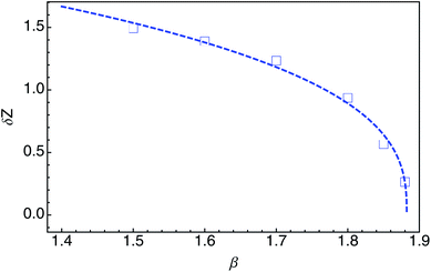Fig. 2 Average δZ as a function of β values, which indicates that the system will reach isostatic point J when β ≈ 1.88.

Of course, simultaneous determination of the location of a critical point and the corresponding exponent is difficult to do precisely. And, we are limited in how closely we can approach the isostatic limit by critical slowing down. Simulations in the vicinity of the isostatic point are very slow to equilibrate; the system becomes increasingly constrained because of the progressive removal of degrees of freedom of the force network in excess of the number required to maintain mechanical equilibrium. Still, it seems clear that the observed behavior of our model is consistent with the isostatic point being reached at a finite value of β ≈ 1.88.

3 Bond force network

3.1 Bond force auto-correlation function

Time–correlation functions, which describe the equilibrium statistics for time evolution of a variable of interest, are an effective and intuitive way of representing the dynamics of a system. Here, we use the multiple-tau correlator method²³ to calculate the force auto-correlation function C_f(t, β, i) = 〈f(τ, β, i)f(t + τ, β, i)〉 of bond i in a system with fictitious reciprocal temperature β. The force on bond i at time t is denoted by f(t, β, i), and 〈 〉 represents a time average in an equilibrated simulation. By averaging as well over all bonds in the system, we obtain C_f(t, β) is defined as , where M is the total number of bonds in the system.

Fig. 3 displays the force autocorrelation function for β = 1.5, 1.55, …1.8 as a log–log plot. The autocorrelation functions decay progressively more slowly as β increases.

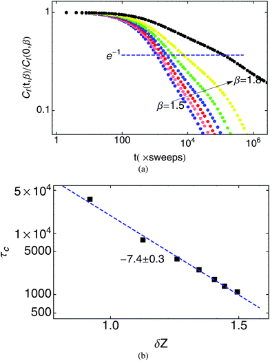Fig. 3 (a) log–log plot of force auto-correlation function for β = 1.5, 1.55, …, 1.8. (b) Characteristic time τ_cversus δZ.

In a force network with few zero bonds (corresponding to small β), nearly any wheel move proposed can be performed, because there are no bonds bearing zero force that would be potentially driven negative, leading to the rejection of the move. However, as system approaches isostatic point, there are nearly as many constraints as there are lattice sites. Thus the probability of a wheel move affecting a zero bond increases, such that almost no wheel moves will succeed, which drastically slows the dynamics of the model.

The decay is reasonably consistent with a power law over intermediate times (10³sweeps < t < 10⁵sweeps). To characterize the growth of the relaxation times with a single value for each β, we arbitrarily select the time for decay of the autocorrelation function to 1/e. We plot these values versus the corresponding average δZ (computed from the average Z̄(β) for each β value), to observe how the timescale grows as we approach the isostatic point. Although we are relatively far from the isostatic limit, we observe power-law growth of the timescale with a rather large exponent, τ_c ∼ δZ^−7.4±0.3 (see Fig. 3(b)).

Evidently, the characteristic timescales for our model grow quite rapidly as the isostatic point is approached. In plotting the timescales log–log against δZ, we are in effect testing the assumption that the timescales diverge at point J (at which δZ → 0). The reasonable fit of a single power law without systematic deviations suggests that this identification of point J with a dynamical transition is correct.

Note also that with such a strong divergence of the timescales, it is quite difficult to approach very near to the transition in this model and carry out an equilibrated simulation. Each factor of two reduction in δZ results in a slowdown by about a factor of 150.

Because the number of wheel moves not prohibited by some zero bond becomes small near point J, continuous-time MC simulations²⁴ become an attractive approach to simulating our model. Briefly, in continuous-time MC, a full list of possible moves and their energy penalties is maintained, organized in groups of moves with exactly the same energy. (Because we have a lattice model, the number of different possible energy changes for any wheel move is manageably small.) Then at each step, a move is selected at random, weighted according to its Boltzmann factor. All moves succeed, and the simulation clock is advanced with an adjustable timestep that ensures detailed balance.

We have employed continuous-time MC simulations to improve the efficiency of our simulations nearer to point J. Even with the overhead of maintaining lists of possible moves, continuous-time MC speeds up our simulations by a factor of about 10 for the largest β values we studied.

3.2 Global dynamics

A commonly employed probe of dynamical response in glassy systems is provided by the mean persistence function,^15,16 defined ashere P_i(t) is the persistence function of bond i defined as the probability that bond i will not change state in a time t; P_i(0) is unity, and approaches zero as t becomes large. Because we are interested in the evolution of the force network, which is evidently slowed by the presence of zero bonds, for simplicity we define the “state” of a bond to be whether the force it bears is zero or nonzero.

We acquire data to compute P_i(t) by keeping track for each bond of the last time the bond changed state (see Fig. 4). Then at any given time, we can compute the time since a given bond last changed state. Because our simulations are microscopically reversible (they satisfy detailed balance), we can interpret the time trajectory of our simulations as a “movie in reverse”. Thus the statistics of the time since a bond last changed state is equivalent to the statistics of the time we must wait until a bond next changes state.

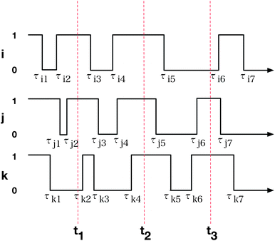Fig. 4 Schematic time-dependence of the “state” of a bond. The m-th state change of bond i is at time τ_im; the nth configuration is recorded at time t_n (see main text).

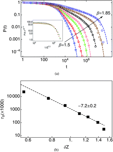
Fig. 5(a) displays a log–log plot of the bond force persistence function P(t) for values of β = 1.5, 1.6, …, 1.85. Again we see that the dynamics of our simulations slow dramatically as the isostatic point is approached. Beyond t ≈ 1000, the persistence functions are reasonably well described by a power-law decay with an exponential cutoff, of the form

P(t) ∼ t^−a exp(−t/τ_b) (3)

in which the exponent a and the cutoff time τ_b both vary with β. For each β, fits of P(t) to the form of eqn (3) are shown as dashed lines in Fig. 5(a). The corresponding a and τ_b values are given in Table 1.

Fig. 5 (a) Persistence function P(t) of bond forces at different β. (Inset: rescaled master curve.) (b) Mean relaxation time τ_b as a function of distance to the isostatic point. The error bar of each data point is smaller than the symbol size.

Table 1 Fitting parameters in eqn (3) for persistence functions at different β

β	δZ	a	τ b (×1000)
1.5	1.50	1.14 ± 0.02	31.6 ± 0.7
1.6	1.39	1.00 ± 0.01	104 ± 3
1.7	1.23	0.72 ± 0.01	272 ± 3
1.75	1.11	0.57 ± 0.01	495 ± 6
1.8	0.94	0.46 ± 0.01	2060 ± 20
1.83	0.77	0.35 ± 0.01	7350 ± 200
1.85	0.57	0.28 ± 0.01	22 090 ± 290

---

The terminal times τ_b grow markedly with the approach to the isostatic point. As shown in Fig. 5(b), the dependence of terminal times on δZ is consistent with a power-law divergence τ_b ∼ δZ^−7.2±0.2. This is reasonably consistent with the strongly diverging timescale derived from the force autocorrelation function (Fig. 3), i.e., both diverge with power laws in the neighborhood of 7. The cutoff time τ_b at smallest δZ(≈0.58) in the figure is slightly under the best fitting, which is probably due to the limitation of the simulation time. Given the relatively narrow range of δZ our simulations can easily access, these results are consistent with a single strongly-diverging longest characteristic time.

3.3 Dynamic heterogeneity

Commonly when a system exhibits dynamics with timescales that diverge as some transition is approached, there is an accompanying divergence in some characteristic spatial scale. For equilibrium second-order phase transitions, the diverging length is the correlation length of the order parameter for the transition. For dynamical transitions in glassy systems, the diverging length scale is less obvious.

Naively, we may wonder if there are growing spatial correlations in the locations of zero bonds in the force network. Note that the location of zero bonds is not strictly random, since their placement must be consistent with static equilibrium at every site. Thus the ensemble described by our lattice jamming model is not simply a randomly pruned lattice.

We may look for spatial correlations between the local density of zero bonds, and the persistence time of nearby bonds. In Fig. 6, typical snapshots at β values of 1.5, 1.6, 1.7, 1.8 are visualized in three ways: (a) with lines for each zero bond, (b) with coloration according to the persistence time of bonds, and (c) with coloration according to the local density of zero bonds. (The zero bond density at each lattice site is defined as the number of zero bonds among the 12 bonds that would participate in a wheel move on this site.)

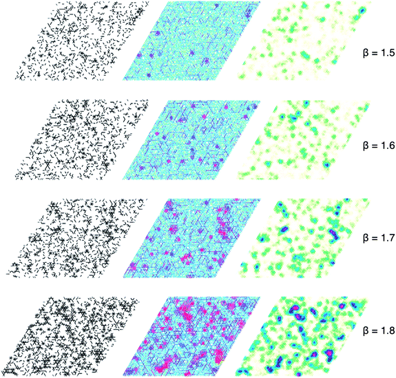Fig. 6 (a) Zero bonds configuration at certain time. (b) Persistence time of bonds. (c) Density of zero bonds.

From Fig. 6, it is clear that the number of zero bonds increases as β increases (as point J is approached), and that the regions which have a greater local density of zero bonds are increasingly slowed down. Although there are more zero bonds at larger β values (smaller δZ), there is no evident growth in the spatial correlation function of zero bond location—indeed, we looked carefully for this in our previous work.²⁰

There is, however, a hint that the spatial extent of regions slowed by a local concentration of zero bonds increases as the isostatic point is approached. To investigate this more quantitatively, we make use of the persistence correlation function commonly used to observe dynamic heterogeneity in simulations of glassy systems.

3.4 Persistence correlations

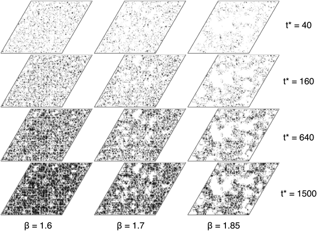
To observe a growing length scale that accompanies the growing dynamical timescales in our lattice model, we make use of the spatial correlations of the local persistence function P_i(t).^15,16

The basic idea of this method is depicted in Fig. 7. In each column of figures corresponding to a given value of β, sites are shown dark if their persistence time (the time interval since the last state change) is less than some selected threshold t*. For small values of the persistence threshold time, only a few scattered sites have changed state. As the threshold time is increased, more and more of the sites have changed state, and eventually the entire frame is dark.

Fig. 7 Spatial distribution of the local persistence of forces at different times for different β.

To place the persistence values on the same triangular lattice as the particles, as well as for later convenience in computing correlation functions, we have averaged the six persistence values of forces acting on a given site to determine a local site-averaged force persistence value. These evidently take on values from the set 0, 1/6, 2/6, …, 1.

As β increases and the dynamics become slow, the threshold time for a given fraction of the sites to change state also increases. We notice that for threshold times such that about half the sites have changed state, spatial correlations become apparent in the location of the changed sites. Furthermore, the length scale for these spatial correlations increases as β increases, and the system comes closer to the isostatic point.

To quantify this growth in this dynamical length scale, we compute the spatial correlation function of the persistence function,¹⁶ defined as

in which 〈 〉 denotes a time average in an equilibrium simulation. The function f(t) = P(t) − P²(t) in the denominator ensures the normalization C(r = 0, t, β) = 1. This correlation function resides on the triangular lattice, but can be most conveniently performed by indexing the lattice as if it were square, and using two-dimensional discrete Fourier transforms and the convolution theorem.

We can also define the discrete Fourier transform of C(r, t), to give the dynamic structure factor of the persistence function,

The zero mode of S(q, t, β) defines a dynamic susceptibility χ(t, β) = S(0, t, β).

Fig. 8 shows the time dependence of the χ(t, β) for different β. The susceptibility develops a peak with increasing amplitude as β increases. The heights of the maximum indicate the spatial extent or ‘strength’ of the heterogeneities. In the figure, the time axis is scaled by a characteristic time t* for each β value, such that the mean persistence function P(t*) equals 1/2, meaning that on the average, half of the bonds have changed state at least once in the time interval t*.

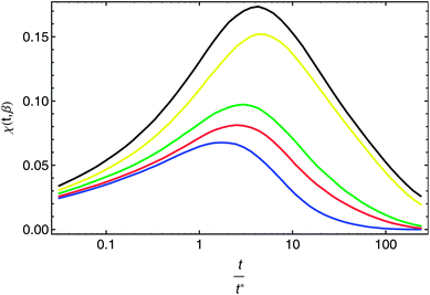Fig. 8 Time dependence of dynamic susceptibility for β = 1.5, 1.6, 1.7, 1.75, 1.8 (from bottom to top).

The conventional prescription for evaluating the persistence correlation function is that the threshold time should be taken to be the time at which χ(t) is maximum, which typically corresponds to t = t* as defined above. Here, as a result of the coarse-graining of the force persistence onto the particle lattice, the peak in χ(t, β) is shifted to slightly longer times, of a few times t*.

In what follows, we have evaluated the persistence correlation functions at the peak time for each β value. Typical configurations are shown in Fig. 9, for β = 1.6, 1.7, 1.8, 1.85. The size of mobile and immobile regions on this timescale steadily increases with increasing β on approach to the isostatic point.

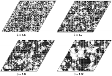Fig. 9 Spatial distribution of local persistence at time t(β) such that χ(t, β) is maximum, for a 60 × 60 system; β = 1.6, 1.7, 1.8, 1.85.

We have obtained persistence correlation functions for different system sizes (L = 30, 60, 120 sites) and find no difference in the results of Fig. 9, indicating that for this range of β and system size, there are no observable finite size effects on the dynamical susceptibilities, which can become a problem when the dynamical clusters become large enough.³⁰

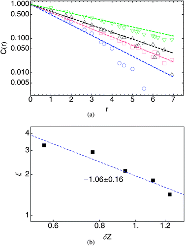
Fig. 10(a) shows the persistence correlation function C(r, t*, β) for different β in a semi-log plot. The correlation length ξ (inverse slope of the plots) grows as β increases and the isostatic point is approached. Although the results are somewhat noisy, Fig. 10(b) shows that growth of ξ is reasonably consistent with a power-law divergence, ξ ≈ δZ⁻¹ as the system approaches isostatic point. (We shall see in the next section that a different measure of the persistence of the force configuration shows a consistent divergence of the correlation length, with better statistics.)

Fig. 10 (a) Spatial correlation function of persistence reveals a growing length scale as the isostatic point is approached. (b) Correlation length scale ξ, as the reciprocal of the slope of fitting, diverges as δZ^{−1.06±0.16} when the system approaches isostatic point J.

4 Reciprocal force tiles

Force networks on a two-dimensional lattice have an interesting dual representation in terms of a reciprocal tiling of the plane, known as the Maxwell–Cremona diagram.^25–27 This reciprocal force tiling provides an alternative representation of the force network,^28,29 and reveals an unexpected conservation law in the dynamics of our model. Here, we briefly reprise the arguments of ref. 28 and 29.

Fig. 11 depicts the bond forces and corresponding force tiles for three typical local configurations. On the left, the particles sit at the intersection of the force arrows, labeled by their integer magnitudes. On the right, the corresponding tiles are shown; each force is rotated clockwise by π/2, and joined head to tail with the neighboring forces. Because each particle is in static equilibrium, the forces must sum to zero, hence the perimeter of the corresponding tile forms a closed (irregular) polygon. Because a site may have one or more zero bonds (any number but five is possible), the reciprocal tile may be a hexagon, pentagon, rhombus, triangle, line, or point.

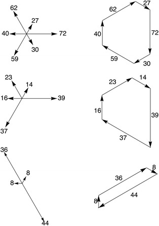Fig. 11 Bond forces (left) and reciprocal force tiles (right) for several typical sites, with different numbers of zero bonds.

Because forces on neighboring sites are equal and opposite, tiles for neighboring sites are consistent with regard to the length of their shared side. In fact, it can be shown that the tiles indeed tile the plane without gaps or overlaps. Clearly, this works for the regular force network, in which all force magnitudes are equal. To show that it works in general, we examine the effect of a wheel move on the reciprocal force tiling, and show that wheel moves change the force tiling in a consistent way. Thus, since the set of wheel moves are ergodic (sufficient to explore the entire ensemble), the tiling is maintained for any configuration of forces that satisfy static equilibrium at fixed average stress.

If we apply a negative wheel move on a given site (Δf = +1 on perimeter bonds and Δf = −1 on radial bonds), the only tiles affected are that of the given tile and its six neighbors. The sides of the reciprocal tiles may be drawn on the bonds of a triangular lattice; the sides of the given tile each move inward by one unit, under the action of the wheel move. This lengthens the sides that separate the neighboring tiles, which correspond to the forces between sites that neighbor the given site, by one unit, just sufficient to preserve the tiling. Hence by the above ergodicity argument, the reciprocal force tiling is always consistent.

Note that under the wheel move dynamics, the total area of the tiling is conserved. If a given tile shrinks under a wheel move, the neighboring tiles grow by the same amount. The area of a tile has dimensions of force squared, and the sum of these values is an unexpected conserved quantity. In the remainder of this section, we will explore the dynamics of the tile area, and investigate the consequences of this conservation law.

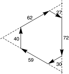
To see how to compute the area of a given tile, consider the example of Fig. 12. The directions of the tile faces lie along the principal directions of a triangular lattice. If we add small equilateral triangles at each corner of the polygon, we recover an equilateral triangle (dashed in the figure), the area of which is A = (1/2)bh = (1/2)sin(π/3)b², where b is the length of one side. We have b = 27 + 72 + 30 (or 30 + 59 + 40, or 40 + 62 + 27). We may then subtract the areas of the small equilateral triangles we added. If we label the bond forces around the tile as {f₁ = 72, f₂ = 30, f₃ = 59, f₄ = 40, f₅ = 62, f₆ = 27}, we may write

Fig. 12 An easy way to calculate the size of tile which is discussed in the text.

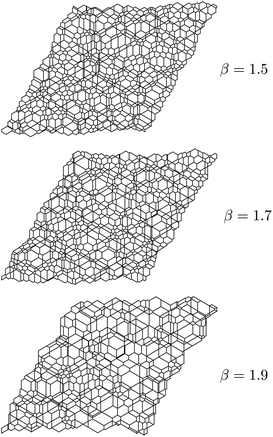
Fig. 13 shows the reciprocal force tiling for typical configurations of a 30 × 30 system with different β values. As β increases and the isostatic point is approached, more tiles with large area are evident. Since the tile area is related to the force magnitudes on the corresponding sites, it is clear that some sites bear much larger forces than others near the isostatic point. The areal density of lines is likewise a visual measure of nonzero forces. The average density of lines at β = 1.9 is smaller than at β = 1.5, consistent with the greater number of zero bonds near the isostatic point.

Fig. 13 Reciprocal force tilings of a 30 × 30 system with β = 1.5, 1.7, 1.9.

4.1 Tile area auto-correlation function

We can investigate the dynamics of our model in terms of the reciprocal tiling, using the same techniques we applied to the direct force network. Here, we examine the autocorrelation function of the tile area for a given site. Since the tile area is quadratic in the forces associated with a given site, the tile area autocorrelation function is the sum of several fourth order auto- and cross-correlation functions of bond forces, while the bond autocorrelation function is simply a second-order correlation function of the forces. Nonetheless, the two types of correlation functions match up surprisingly well, as shown in Fig. 14 for β = 1.5, 1.7, 1.75, 1.8.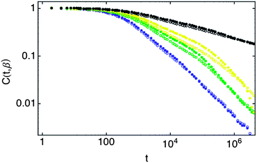

Fig. 14 Comparison between bond force auto-correlation functions (solid) and tile area auto-correlation functions (open) with β = 1.5 (blue), 1.7 (green), 1.75 (yellow), 1.8 (black).

4.2 Persistence function

For the persistence function of reciprocal force tiles, we adopt a different definition than we used for the bond forces. For the bonds, we were most concerned with whether or not a bond bears no force; in contrast, the only tiles with zero area correspond to “rattler” sites with all zero forces. So we define the state of a force tile in such a way as to detect “large” changes in tile area.

For our simulations, we used an initial force value of 24, which corresponds to an initial tile area of 1500. We take this to be the unit of tile area, A₀. As the simulation progresses, the tile areas vary considerably. We define the state of a force tile as its area in units of A₀ to the nearest integer. We keep track of the most recent time the state of each force tile has changed, and proceed on this basis to evaluate P_i(t) and P(t) as for bond forces.

Fig. 15(a) displays the resulting tile area persistence functions P(t), which behave in a similar fashion to the bond force persistence functions. The dynamics slow dramatically as the system approaches the isostatic point. We again use eqn (3) to fit the tile area persistence functions, shown as the dashed lines in Fig. 15(a), with corresponding parameters in Table 2.

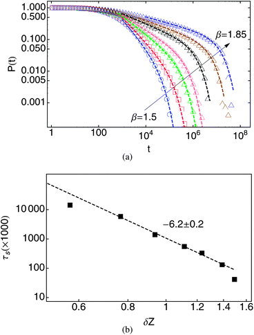Fig. 15 (a) Persistence function P(t) of force tiles for β = 1.5, 1.6, …, 1.85. (b) Mean persistence time τ_s (symbols) versus δZ. The error bar of each data point is smaller than the symbol size.

Table 2 Fitting parameters in eqn (3) for tile area persistence functions

β	δZ	a	10^−3τs
1.5	1.50	0.88 ± 0.02	42 ± 1
1.6	1.39	0.78 ± 0.01	130 ± 3
1.7	1.23	0.58 ± 0.01	328 ± 5
1.75	1.11	0.47 ± 0.01	552 ± 8
1.8	0.94	0.32 ± 0.01	1400 ± 30
1.83	0.77	0.27 ± 0.01	5840 ± 150
1.85	0.57	0.21 ± 0.01	14240 ± 350

---

The relaxation time τ_s diverges as δZ^−6.2±0.2 as we approach the isostatic point, as shown in the log–log plot of Fig. 15(b). Comparing Fig. 15 with the corresponding relaxation times for the bond force persistence function of Fig. 5, we see that the relaxation times from both bond force and tile area display roughly consistent scaling behavior as the isostatic point is approached, i.e., all three determinations of a characteristic time diverge strongly as δZ vanishes, with exponents in the range of 6–7 or so.

In the same manner as for the local persistence of the state of bonds, here we determine a length scale for dynamic heterogeneity based on the spatial correlations of the persistence of the state of force tiles. In this case, perhaps because we perform no coarse-graining, it turns out that the maximum of the susceptibility χ(t) is located almost exactly at t*, the timescale at which the average tile persistence is 1/2. Thus for tile persistence, we make the conventional choice to evaluate the correlation function for a time delay of exactly t*.

Typical figures that result are shown in Fig. 16, for β = 1.6, 1.65, …, 1.85. The size of mobile and immobile regions on this timescale steadily increases with increasing β, on approach to the isostatic point.

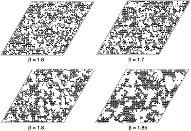Fig. 16 Spatial distribution of local persistence at time t* such that P(t*) = 1/2, for a 60 × 60 system.

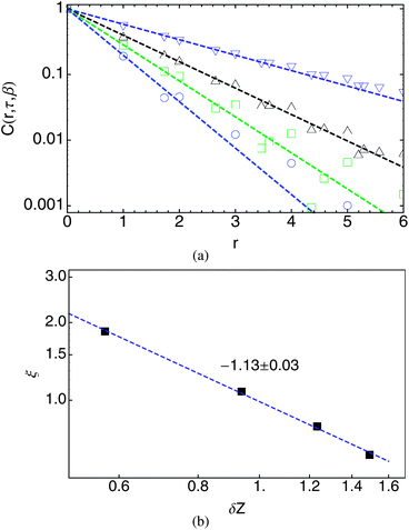
Fig. 17(a) shows the resulting persistence correlation function C(r, t*, β) for different β in a semi-log plot. The correlation length ξ grows as β increases and the isostatic point is approached; ξ exhibits a power-law divergence in the isostatic limit, as ξ ≈ δZ^−1.13, roughly consistent with the modest power-law divergence of the dynamical heterogeneity length scale as defined by the persistence of the state of bonds (see Fig. 10).

Fig. 17 (a) Spatial correlation function of persistence reveals a growing length scale as the isostatic point is approached. (b) Correlation length scale ξ, as the reciprocal of the slope of fitting, diverges as δZ^{−1.13±0.03} when the system approaches isostatic point J.

4.3 Dynamic structure factor of tile area

As remarked above, the reciprocal tile area is a conserved quantity under the wheel move lattice dynamics, which is sufficient to explore the ensemble of force configurations satisfying static equilibrium on all sites, with a fixed average stress. Thus the conservation law is in some sense a property of the ensemble. Here, we examine the consequences of this conservation law, by computing the time correlation of different Fourier modes of the tile area as a function of position, which is to say the tile area intermediate structure factor.

We define the discrete Fourier transform A_k(t) of the local tile area A_j(t) as follows:

where A_j(t) is the tile size of site j at time t, and L is the linear dimension of the simulation array. For computing the discrete transform, we may regard the sites as occupying a square lattice, and the reciprocal lattice labeled by k as likewise square, whereupon each component of j and k is an integer between 0 and L − 1. The corresponding physical wavevector q lives on a triangular reciprocal lattice, given in terms of k_x and k_y by q = k_xe₁ + k_ye₂. Here e₁ = {0, 1} and are the dual basis vectors of the reciprocal lattice.

The time auto-correlation function C(q, t) = 〈A_k(t′)A_k(t + t′)〉 describes how fluctuations at a given wavevector decay in time. The simplest behavior of such a function is exponential decay of each mode, with a q-dependent relaxation time τ(q). Because the tile area is conserved, we expect that the relaxation time τ(q) should be proportional to at least q⁻², reflecting the fact that fluctuations at long wavelengths λ = 2π/|q| decay slowly because of the need to transport excess tile area to distant locations of order λ away.

Our lattice model has hexagonal symmetry, so we expect that values of the correlation function corresponding to wavevectors related by rotation by 2π/6 should be equivalent. More generally, at length scales long compared to the lattice dimension, we expect our model to be isotropic. Hence in presenting results for C(q, t) we first average over equivalent wavevectors, and then present the results only as a function of wavenumber, as C(q, t).

Fig. 18 presents a log–log plot of the intermediate structure factor C(q, t) for selected q values (q = 1, 2, 4, 8, 16) and β values (β = 1.5, 1.6, 1.7, 1.8). For β values other than β = 1.8 (nearest to the isostatic point), the individual autocorrelation functions decay approximately exponentially, with characteristic timescales τ(q; β) that are longer at low q and for larger β, as expected.

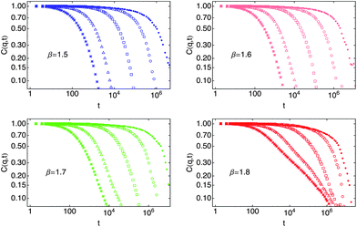Fig. 18 Tile area intermediate structure factor C(q, t) with β = 1.5, 1.6, 1.7, 1.8 in a 30 × 30 system, for q = 1 (•), 2 (○), 4 (□), 8 (Δ), 16 (*).

Our results for β = 1.8 deviate from this pattern, particularly at higher q and at later times. It is not immediately clear whether this is an artifact of an incompletely equilibrated system or a consequence of the approach of the isostatic point.

To quantify the dependence on q and β of the relaxation, we have defined correlation times as the time for C(q, t) to decay to 1/e. The resulting values are shown in Table 3.

Table 3 τ _q at different q and β where C(q, τ_q) = e⁻¹

q	β
	1.5	1.6	1.7	1.8
2	260	460	790	3300
4	25	38	59	280
8	1.8	2.9	4.2	31

---

Fig. 19(a) displays a log–log plot of τ(q) versus q for different β, in which it is clear that the k-dependence of the relaxation times is well described for all β by a power law, τ(q) ∼ q^−3.6±0.1.

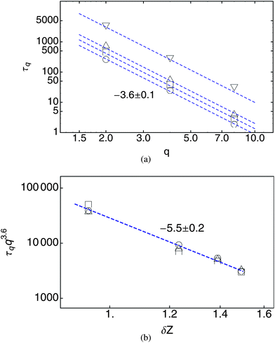Fig. 19 (a) τ(q) for β = 1.5 (○), 1.6 (□), 1.7 (Δ) and 1.8 (∇). (b) τ(q)q^3.6versus δZ for systems with different β values, well described by scaling dependence δZ^−5.5±0.2.

With the q dependence of τ(q) determined, we can examine the dependence of τ on the distance δZ to the isostatic point, by plotting τq^3.6versus δZ in a log–log plot (see Fig. 19(b)). Again we find a power-law dependence, this time with τ_qq^3.6 diverging as δZ^−5.5±0.2. Combining these scaling results, it appears the tile area autocorrelation times scale as

τ_q ∼ q^−3.6±0.1δZ^−5.5±0.2 (8)

Now we plot the correlation functions C(q, t) versus tq^3.6δZ^5.5, whereupon a reasonable master curve results (see Fig. 20).

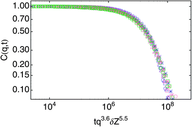Fig. 20 C(q, t) versus tq^3.6δZ^5.5 produces a master curve for β = 1.5 (blue), 1.6 (pink) and 1.7 (green).

5 Conclusions

We have devised a lattice model to study dynamics of force networks in jammed granular solids. Using a biased Monte Carlo (MC) simulation, we can tune the number of bonds in the network that bear no force, and hence the distance from the isostatic point. The lattice structure of our model permits us to use simple Monte Carlo moves and grants us access to simple mathematical analyses of the resulting configurations, both advantages not afforded by geometrically random systems. The ensemble explored by our lattice simulation can be identified with a collection of packings of stiff, nearly spherical but slightly rough particles, which pack on a triangular lattice. The contacts between particles bear different forces at fixed average pressure, because of the slightly different particle radii along each contact. All forces are either repulsive or zero.

Our simulation makes use of previous work of Tighe et al., who introduced a “wheel move” for changing the forces acting on a given site and its neighbors, in such a way as to maintain force balance on all sites. There is one wheel move per lattice site—the same as the number of force bonds in excess of the number required to satisfy static equilibrium on each site. The wheel moves are all linearly independent, and therefore sufficient to explore the ensemble of force configurations.

Because the forces are required to be nonnegative, any wheel move that would lead to negative forces between particles is prohibited. As our biased MC simulation depletes the system of force-bearing bonds, an increasing fraction of wheel moves are not permitted. This leads to dramatic slowing of the dynamics as we approach the isostatic point.

This present work focuses on the dynamics of our simulation, and how various characteristic timescales diverge as the isostatic point is approached. We investigate the autocorrelation function of bond forces, and the distribution of persistence times for the “state” of bonds (defined as the time to wait until a nonzero bond becomes zero, or vice versa). Over the limited range of δZ accessible to our simulations, these different characteristic times all show strong divergences with distance from the isostatic point, with power laws around −6 to −7. Such strong divergences place practical limits on how close to the isostatic point we can approach with a well-equilibrated simulation.

As explained above, the strong slowing of the dynamics results from the increasing prevalence of zero bonds in the system. The zero bonds themselves do not exhibit any marked tendency to cluster, and their concentration shows no long-range correlations as we approach the isostatic point. As with other glassy dynamical systems, a growing length scale can be observed by computing the spatial correlation function of the “persistence probability”, i.e., the likelihood that a given site has changed state. In a given configuration, sites that are “mobile” or “frozen” tend increasingly to cluster as the system slows down. The correlation length diverges as a power law of about δZ⁻¹ when the system approaches isostatic point J.

Our lattice model of forces has a dual representation as a reciprocal tiling of the plane, in which each site corresponds to a polygon with sides equal in length to the dual force. Because the wheel move preserve the force balance and conserve the stress, the total area of the reciprocal tiles is conserved by our dynamics. We investigate the consequences of this conservation by computing the intermediate structure factor for the local tile area. We find the wavenumber-dependent relaxation time τ(q) scales with wavenumber as q^−3.6±0.1 over a range of distances from isostaticity, with a prefactor that diverges as δZ^−5.5±0.2 as the isostatic point is approached.

In future work, there are several approaches we can pursue to increase the dynamic range of our simulations, and so explore the diverging dynamic length and time scales more thoroughly. First, we can reduce the average force value (here f₀ = 24), to something smaller (e.g., f₀ = 4). Since each wheel move only changes the forces by one unit, much time is spent in what amounts to 1d diffusion of the force values. We surmise that the “uninteresting” time range in the persistence functions between t = 1 and t = 500 or so (see Fig. 5(a) and 15(a)) results from this 1d diffusion, scaling as f₀². Reducing f₀ by a factor of six would then give perhaps 1.5 more usable decades in time.

Also, our simulations here are all single-processor; however, we could apply shared-memory parallelization using OpenMP. We could partition a lattice of size 60 × 60 into a 5 × 5 array of regions of 12 × 12 sites, each of which is further divided into a 3 × 3 array of 4 × 4 areas. We could then employ 25 processors to simultaneously propose wheel moves, each chosen from within corresponding 4 × 4 areas within each region (this avoids any interference between moves). Continuous-time MC would be problematic to implement with multiple processors, because changes in the list of possible moves as a result of a move alter the probabilities with which subsequent moves are to be selected. However, CTMC only gave us a 10× speedup at the largest β values, so simple Metropolis with multiple processors could be competitive.

Although the strong power-law divergence of dynamical timescales in our lattice model limit how closely we can approach the isostatic point, our results are consistent with a power-law divergence of timescales at the isostatic point, which appears to be reached in our model at an effective temperature of about β ≈ 1.9 (Fig. 2). This dynamic transition is not accompanied by an evident diverging correlation length in some static order parameter, but only by diverging length scales associated with dynamic heterogeneity. Thus this Hamiltonian-based model appears to display an important hallmark of a glass transition at finite control parameter.

Acknowledgements

The authors acknowledge support from NSF DMR-0907370 and ACS PRF 49964-ND7.

References

1. P. W. Anderson, Science, 1995, 267, 1615.
2. M. Ediger, Annu. Rev. Phys. Chem., 2000, 51, 99.
3. E. R. Weeks, J. C. Crocker, A. C. Levitt, A. Schofield and D. A. Witz, Science., 2000, 287, 627.
4. A. Heuer and K. Okun, J. Chem. Phys., 1997, 106, 6176.
5. D. N. Perera and P. Harowell, J. Non-Cryst. Solids, 1998, 235, 314.
6. C. Donati, et al. , Phys. Rev. Lett., 1998, 80, 2338.
7. A. Liu and S. Nagel, Nature, 1998, 396, 21.
8. V. Trappe, V. Prasad, L. Clpelletti, P. N. Segre and D. A. Weltz, Nature, 2001, 411, 772.
9. P. J. Lu, E. Zaccarelli, F. Ciulla, A. B. Schofield, F. Sciortino and D. A. Weltz, Nature, 2008, 453, 499.
10. K. Stratford, R. Adhikari, I. Pagonabarraga, J. C. Desplat and M. E. Cates, Science, 2005, 309, 2198.
11. M. van Hecke, J. Phys.: Condens. Matter, 2010, 22, 033101.
12. C. O'Hern, S. Langer, A. Liu and S. Nagel, Phys. Rev. Lett., 2002, 88, 075507.
13. C. O'Hern, L. Silbert, A. Liu and S. Nagel, Phys. Rev. E: Stat., Nonlinear, Soft Matter Phys., 2003, 68, 011306.
14. H. Sillescu, J. Non-Cryst. Solids, 1999, 243, 81.
15. E. Bertin, J.-P. Bouchaud and F. Lequeux, Phys. Rev. Lett., 2005, 95, 015702.
16. S. Whitelam, L. Berthier and J. P. Garrahan, Phys. Rev. E: Stat., Nonlinear, Soft Matter Phys., 2005, 71, 026128.
17. J. H. Snoeijer, T. J. H. Vlugt, M. van Hecke and W. van Saarloos, Phys. Rev. Lett., 2004, 92, 054302.
18. T. Unger, J. Kertesz and D. E. Wolf, Phys. Rev. Lett., 2005, 94, 178001.
19. B. Tighe, J. Socolar, D. Schaeffer, W. Mitchener and M. Huber, Phys. Rev. E: Stat., Nonlinear, Soft Matter Phys., 2005, 72, 1.
20. J. Newhall, J. Cao and S. T. Milner, Phys. Rev. E: Stat., Nonlinear, Soft Matter Phys., 2013, 87, 052203.
21. G. H. Fredrickson and H. C. Andersen, Phys. Rev. Lett., 1984, 53(13), 1244.
22. G. H. Fredrickson and H. C. Andersen, J. Chem. Phys., 1985, 83(11), 5822.
23. J. Ramirez, S. K. Sukumaran, B. Vorselaars and A. E. Likhtman, J. Chem. Phys., 2010, 133, 154103.
24. M. E. J. Newman and G. T. Barkema, Monte Carlo Methods in Statistical Physics, Clarendon Press, Oxford, 1999.
25. J. C. Maxwell, Philos. Mag., 1864, 27, 250.
26. R. Satake, Mech. Mater., 1993, 16, 65.
27. R. C. Ball and R. Blumenfeld, Phys. Rev. Lett., 2002, 88, 115505.
28. B. P. Tighe, A. R. T. van Eerd and T. J. H. Vlugt, Phys. Rev. Lett., 2008, 100, 238001.
29. B. P. Tighe and T. J. H. Vlugt, J. Stat. Mech.: Theory Exp., 2010, P01015.
30. S. Karmakar, C. Dasgupta and S. Sastry, Proc. Natl. Acad. Sci. U. S. A., 2009, 106, 3675.

---