 Open Access Article
 This Open Access Article is licensed under a Creative Commons Attribution-Non Commercial 3.0 Unported Licence
Focusing of mammalian cells under an ultrahigh pH gradient created by unidirectional electropulsation in a confined microchamber†
Despina Nelie
Loufakis
a,
Zhenning
Cao
b,
Sai
Ma
b,
David
Mittelman
c and
Chang
Lu
*ab
aDepartment of Chemical Engineering, Virginia Tech, Blacksburg, Virginia 24061, USA. E-mail: changlu@vt.edu; Fax: +1 540 231 5022; Tel: +1 540 231 8681
bSchool of Biomedical Engineering and Sciences, Virginia Tech-Wake Forest University, Blacksburg, Virginia 24061, USA
cVirginia Bioinformatics Institute and Department of Biological Sciences, Virginia Tech, Blacksburg, Virginia 24061, USA
First published on 9th June 2014
Abstract
The transport and manipulation of cells in microfluidic structures are often critically required in cellular analysis. Cells typically make consistent movement in a dc electric field in a single direction, due to their electrophoretic mobility or electroosmotic flow or the combination of the two. Here we demonstrate that mammalian cells focus to the middle of a closed microfluidic chamber under the application of unidirectional direct current pulses. With experimental and computational data, we show that under the pulses electrochemical reactions take place in the confined microscale space and create an ultrahigh and nonlinear pH gradient (∼2 orders of magnitude higher than the ones in protein isoelectric focusing) at the middle of the chamber. The varying local pH affects the cell surface charge and the electrophoretic mobility, leading to focusing in free solution. Our approach provides a new and simple method for focusing and concentrating mammalian cells at the microscale.
Introduction
Proteins and peptides have both amine and carboxylic acid groups and these groups can either donate or accept protons. Therefore the charge of a protein/peptide molecule varies with the surrounding pH. The pH value at which a protein molecule carries no net surface charge is referred to as the isoelectric point (pI) and is an important physiochemical property. Isoelectric focusing (IEF) has been widely used for protein concentration and separation.1,2 In these experiments, carrier ampholytes (i.e. a mixture of molecules with multiple aliphatic and carboxylate groups) or acrylamido buffers (typically covalently incorporated into the gels) are used to establish a linear pH gradient in gels or capillary tubes. A direct current (dc) field is then applied to focus various molecules to their respective pI values. IEF has also been applied to small bioparticles3 (with diameters <5 μm) such as viruses,4,5 bacteria,6,7 and yeasts.8 In these works, special care was taken to use very low concentrations for these bioparticles to avoid interference due to the interactions between the bioparticles and the ampholyte matrix.8 IEF of mammalian cells (with diameters typically in the range of 10–20 μm) on a simple and practical platform has yet to be demonstrated, due to the potential cell entrapment in matrices.The surface charge of mammalian cells is typically negative at physiological pH. Cells are covered by a surface coat that is rich in carbohydrate, referred to as glycocalyx. These carbohydrates include oligosaccharide chains covalently bound to membrane proteins (glycoproteins) and lipids (glycolipids).9 The carbohydrate portion of these molecules contains a significant amount of sialic acid residues that carry negative charges at physiological pH.10–12 At the same time, the carbohydrate groups also contain amino sugars which may become positively charged under low pH.10,11 Thus we hypothesized that concentration or focusing of mammalian cells under a very high pH gradient would be potentially feasible. Such method may find applications in microfluidic total analysis systems that require cell manipulations.13–16
Here, by exploiting the interplay among microfluidics, electrochemistry, and electrokinetics, we demonstrate IEF of mammalian cells in a simple microfluidic electrochemical chamber containing a low-conductivity buffer. We observed focusing of cells in a closed microfluidic chamber when unidirectional pulses were applied by two surface electrodes. Our experimental and computational results show that an ultrahigh pH gradient (up to 0.14 Unit per μm) was generated by electrolysis of water inside the confined microscale space under the application of the electric pulses. The pH gradient was highly nonlinear and steepest at the center of the chamber. We also studied the correlation between the electrophoretic mobility of cells and the local pH and estimated the pI of Chinese hamster ovary (CHO) cells to be in the range of 4.5–6.5. Our setting offers a simple approach to generate an ultrahigh pH gradient at microscale in free solution. Such conditions uniquely permit the focusing of mammalian cells without involving matrices.
Results and discussion
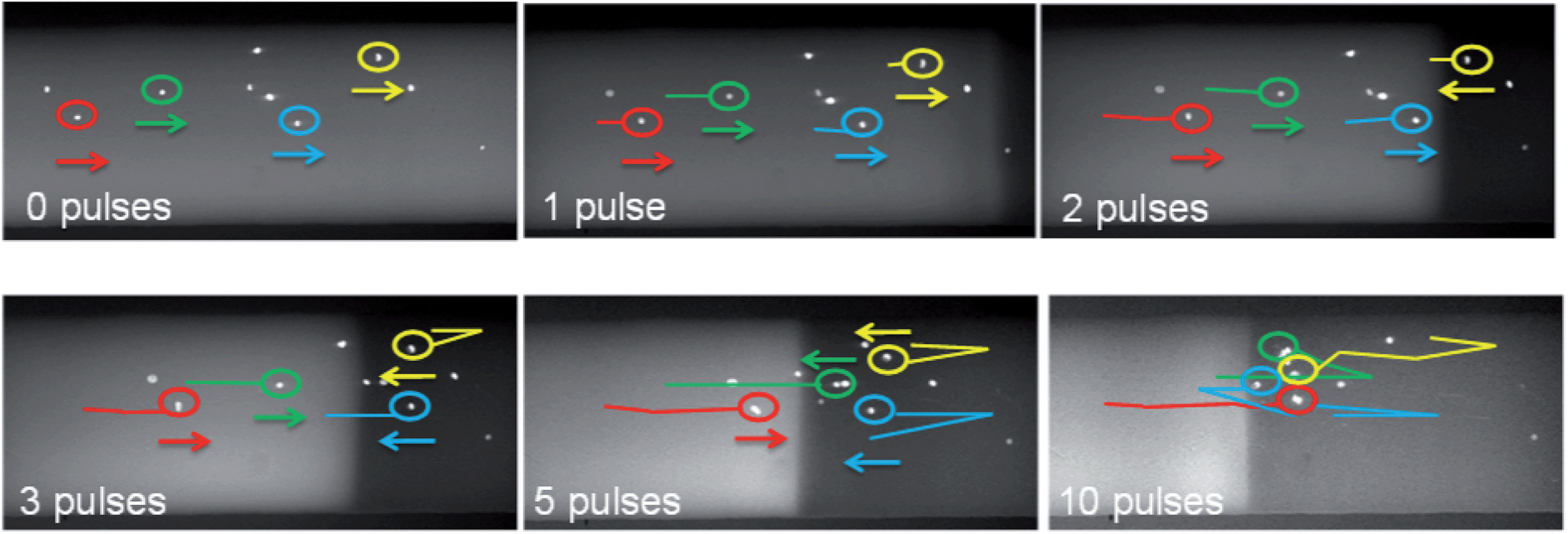
The microfluidic device used in our study is shown in Fig. 1A and ESI Fig. S1.† Cells (typically 10–150) were loaded into a microfluidic chamber of 1.5 mm × 400 μm × 13 μm. These cells were sealed inside the chamber by closing the pneumatic valves at the two ends. Two long planar gold electrodes (120 μm wide, and 1 mm apart) were inside the chamber and 30 ms-long dc pulses were applied via these electrodes every 10 s for 50 times with the pulse intensity in the range of 400–1800 V cm−1. CHO cells were initially tested. Interestingly, under unidirectional pulses, the cells did not move in a consistent direction. The cells eventually focused into a narrow region around the center of the chamber (Fig. 1B and ESI Video S1†). Such movement could be tracked by both phase contrast imaging and fluorescence imaging (after labeling the cells with Hoechst 33342 which penetrates the cell membrane and intercalates within their DNA). In general, the focusing of the cells became more rapid when higher field intensity pulse was used (in the range of 400–1800 V cm−1). The cells finished focusing after 50 pulses under 1000 V cm−1 while the same process essentially was completed after 10 pulses of 1800 V cm−1. Fig. 1C reveals that in general, high pulse intensity also led to improved focusing. For example, a 1000 V cm−1 or higher field intensity was required for complete focusing of cells within a ∼30 μm-wide region. | ||
| Fig. 1 The focusing of cells in a closed microfluidic chamber under unidirectional electropulsation. (A) The design of the closed microfluidic chamber. The microfluidic chamber (1.5 mm × 400 μm × 13 μm) was confined by two pneumatically actuated valves during electropulsation. Square pulses were applied to the system via two surface gold electrodes. (B) Time-lapse images of CHO-K1 cell focusing under 50 pulses of various field intensities (400, 1000, and 1800 V cm−1). Each pulse was 30 ms in duration and rectangular and occurred at the beginning of a 10 s duration (i.e. the interval between pulses was 9.97 s). In the fluorescent images, the cells were stained by Hoechst 33342. A buffer system containing 4.8 mM Na2HPO4, 1.2 mM KH2PO4, and 250 mM sucrose was used. (C) The effect of the field intensity E of the pulses on the standard deviation in the cell locations along X axis after 50 pulses. | ||
Next, we analyze the mechanistic details involved in such isoelectric focusing of mammalian cells. The use of a closed microscale chamber in our design amplified the impact of electrochemical lysis of water. Hydroxides were generated at the cathode (the negative terminal) and protons were produced at the anode (the positive terminal) under sufficiently high voltage. Thus during the course of electropulsation, the local pH at the cathode became basic while the pH close to the anode turned acidic. The generation of a pH gradient under this mechanism was a significant process given the tiny volume of the microfluidic chamber. We conducted COMSOL modeling to examine the electrochemical process. A couple of simplifications needed to be made in order for the modeling to converge. First, we neglected the electrophoresis of ions. We will discuss the implications of this simplification below. Second, we considered only two important reactions (neutralization between H+ and OH− and conversion between the anions in the buffer H2PO4− and HPO42−). The other reactions associated with phosphoric acid and phosphate anion are only important in extreme pH (<3 or >12, respectively), thus have smaller impact on the buffering.
We modeled three buffer concentrations under the application of 50 pulses (each with a 30 ms duration and 1000 V cm−1 intensity): (1) [HPO42−] = 0, [H2PO4−] = 0 (Fig. 2A); (2) [HPO42−] = 4.8 mM, [H2PO4−] = 1.2 mM (Fig. 2B); (3) [HPO42−] = 9.6 mM, [H2PO4−] = 2.4 mM (Fig. 2C). As presented in the inset graphs of Fig. 2A–C, after the first pulse (with the onset at t = 0 and a duration of 30 ms) at t = 0.04 s, hydroxides and protons are generated at the locations of the electrodes inside the chamber. These ions then diffuse during the interval between the first and second pulse (9.97 s) into the rest of the chamber volume, forming a sharp pH gradient close to the center of the chamber. Such pH gradient continues to increase with the application of first several additional pulses. In all three cases, the pH profile reaches its steady state after roughly the first 10 cycles (with one cycle referring to one 30 ms pulse followed by 9.97 s interval). After reaching the steady state, the pH profile still experiences the dynamics caused by the production of protons and hydroxides by additional pulses. However, the pH profile at the end of each additional cycle is identical. With increasing buffer concentrations, the pH profile in the chamber shows more resistance to pulse-induced pH change. Furthermore, the buffer in general has more buffering power in the acidic region (the right side of the chamber) than in basic region (the left side of the chamber) due to the higher starting concentration for HPO42− (4 times higher than that of H2PO4−).
 | ||
| Fig. 2 The formation of pH gradient due to water electrolysis. The pH profiles along the length of the microfluidic chamber (x axis) at multiple time points are computed by COMSOL Multiphysics for three buffer concentrations (A) no buffer, (B) 4.8 mM Na2HPO4, 1.2 mM KH2PO4, and (C) 9.6 mM Na2HPO4, 2.4 mM KH2PO4. The cathode is located at x = 130–250 μm, the anode is located at x = 1250–1370 μm, and both electrodes are 120 μm wide. The pulses are applied once every 10 s and last for the first 30 ms of each 10 s cycle (e.g. in the first cycle, the pulse lasts during t = 0–0.03 s). The insets show the pH profile change during the first cycle (t = 0–10 s). | ||
Electrophoresis of ions affects the pH profile. The electrophoresis of protons and hydroxides only has minor impact on the location of the neutral pH interface in the middle of the chamber. On the other hand, the electrophoresis of HPO42− and H2PO4− may have more significant influence on the pH profile. The majority of these anions is swept to the right side of the chamber after the first 4 cycles by electrophoresis and stay there for the rest of the process, as shown in ESI Fig. S2.† Thus, after the first 4 cycles, the buffering effect is primarily present on the right side of the chamber (with roughly doubled buffer concentration) while the left side of the chamber has few buffering ions.
To summarize, the actual pH profiles in the chamber over the course of the 50 cycles are best described by mixing the results under various buffer concentrations shown in Fig. 2. For a buffer with the concentration of [HPO42−] = 4.8 mM and [H2PO4−] = 1.2 mM (which was used in most of our experiments), the pH profiles are similar to the ones in Fig. 2B for the first 4 cycles. Then for cycles 5 to 50, the left side of the pH profiles will be similar to those in Fig. 2A and the right side will be similar to those of Fig. 2C. The pH gradient forms in the chamber in spite of the presence of the buffer. The buffer provides some resistance to the pH change within the initial 10 cycles, with such buffering effect more pronounced on the right side than on the left side. The location of cell focusing observed experimentally (at x = ∼750 μm, as shown in Fig. 1B) matches the location of the steep pH gradient suggested by the modeling when the buffer is considered (Fig. 2B and C).
Based on the data generated by the modeling, we estimate that a pH gradient of 0.07 Unit μm−1 was formed after the first pulse and it reached and stabilized at ∼0.14 Unit μm−1 after the 10th pulse (Fig. 2B) at a location around the center of the chamber. Such a pH gradient was roughly 2 orders of magnitude steeper than that in the typical protein IEF setting (between 0.001 and 0.2 unit per 100 μm5,17–19). The anode pH decreased from 7.4 to 3.8 after the first pulse and further to 2.0 after the 10th pulse. Similar trend was observed at the cathode where the pH became 11.6 after the first pulse, and increased to 12.2 after the 10th pulse. At the steady state (after 10th pulse), a pH range of 3.8 to 10.5 was covered in a narrow 50 μm distance along x.
The establishment and dynamics of the pH gradient could be observed experimentally by having fluorescein dissolved in the buffer. Fluorescein is pH-sensitive and its fluorescence reduces significantly in acidic environments (e.g. the fluorescence intensity of fluorescein decreases by about 70% as the pH changes from 10 to 5, due to its protonation20). ESI Fig. S3† shows that the fluorescence on the right side of the chamber (close to the anode) started to disappear with the application of the pulses. The boundary (between the dark and fluorescent areas) continued to recede to the left as more pulses were applied. The boundary eventually stabilized after ∼15 pulses at a location on the left side to the center of the chamber. Electrophoresis of the negatively charged fluorescein (with a mobility of −10 to −25 × 10−9 m2 V−1 s−121) did not affect the location of the fluorescence boundary because electrophoresis moved these molecules to the right side of the chamber (which was acidic and effectively quenched the fluorescence). In addition, there might also be contribution from electrochemical processes that caused fluorescence quenching at the right side of the chamber (e.g. Kolbe electrolysis on the anode22). Thus the shift of the fluorescence boundary to the left end of the chamber roughly reflected the dynamic change in the pH inside the chamber. We found that having the interval (between pulses) at 9.97 s was necessary to allow enough time for gas bubbles generated at the electrodes to dissipate through PDMS.23 When the interval was much shorter (e.g. 0.97 s, as in ESI Fig. S3†), there was instability in the boundary, presumably due to the accumulated bubbles on the electrodes. Thus we used 9.97 s intervals for all other experiments that applied consecutive pulses.
Close observation reveals that the cell movement had close correlation to its location relative to that of the fluorescein boundary which roughly separated the acidic and basic regions. In Fig. 3, we show the movement of both the fluorescein boundary (by having fluorescein in the buffer) and the cells during the first 10 pulses. At the beginning of the process, and before the first pulse, the solution had a slightly basic pH (7.4). Thus initially all cells were negatively charged and moved toward the anode (in the reverse direction of the applied field). However, after the first 2 pulses a significant region close to the anode turned acidic (indicated by the loss of fluorescein fluorescence). This led to a change in the moving direction for these cells, causing them to move towards the cathode. It is worth noting that cells stabilized when they crossed 10–20 μm over the fluorescein boundary line to the right, indicating that the neutralization in the cell surface charge occurred under a low pH. For the cells which were at the far left of the boundary line, they experienced only movement toward the right (anode) due to the fact that they were always under the basic pH. The effect of electroosmotic flow in here can be ignored as the chamber was closed during the process. The similar movement trajectories of cells can also be seen in ESI Video S2.†
 | ||
| Fig. 3 Time-lapse images that show the movement of cells inside the chamber in relation to the boundary formed by fluorescein. The cells were stained by Hoechst 33342 and suspended in the buffer containing fluorescein. A buffer system containing 4.8 mM Na2HPO4, 1.2 mM KH2PO4, and 250 mM sucrose was used. The pulses (1000 V cm−1) were applied once every 10 s and lasted for the first 30 ms of each 10 s cycle. | ||
It is interesting to track the dynamics in the electrophoretic mobility of a cell under the pulse sequence and the local pH at the moment. The pH varied with the location inside the chamber and the number of pulses that have been exerted. We calculated the local pH values for cells at a particular moment based on our COMSOL modeling and tracked the corresponding velocity, and therefore the electrophoretic mobility, based on the videometric data. Fig. 4 shows that the local pH strongly affected both the direction and magnitude of the electrophoretic mobility. First of all, all cells moved from the cathode to the anode (shown with negative sign) when pH was higher than 6.5 (with an average μ of −19.86 mm2 kV−1 s−1 and a standard deviation of 8.01 mm2 kV−1 s−1), whereas the vast majority of the mobilities were positive when the pH was lower than 4.5 (the average value of μ was 1.68 mm2 kV−1 s−1 and the standard deviation was 4.20 mm2 kV−1 s−1). This confirms that cells were negatively charged at high pH and positively charged at low pH with a threshold range of pH 4.5–6.5 separating the two regimes. This fairly wide range for pI may be related to the heterogeneity in the cell population. Other than pH, mechanisms such as cell polarization in the electric field may also have effect on the distribution of the cell surface charge and the electrophoretic mobility.24
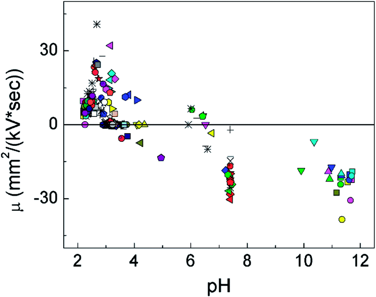 | ||
| Fig. 4 The effect of the local pH on the electrophoretic mobility of a cell during a pulse. The pH of the solution at various time points and physical locations (inside the chamber) was determined using COMSOL Multiphysics. The electrophoretic mobility of cells was calculated after measuring the velocity of cells (i.e. the distance it traveled during the pulse divided by the pulse duration) under an specific field intensity (i.e. 1000 V cm−1). Each individual cell is represented by a specific type of markers. The pulses were applied once every 10 s and lasted for the first 30 ms of each 10 s cycle. A buffer system containing 4.8 mM Na2HPO4, 1.2 mM KH2PO4, and 250 mM sucrose was used. | ||
We also tested various buffer concentrations (2.4 mM Na2HPO4–0.6 mM KH2PO4, 4.8 mM Na2HPO4–1.2 mM KH2PO4, and 8 mM Na2HPO4–2 mM KH2PO4) experimentally (ESI Fig. S4†). The results indicate that the mobility of cells was not significantly affected by the buffer concentration in this range. This confirms that the buffering power of the solution was not enough to counteract the generation of protons and hydroxides by the electrochemical reactions.
Our device and setup allow IEF of mammalian cells of various types and various concentrations (we show IEF of Jurkat cells at high and low concentrations in ESI Fig. S5†), owing to the ultrahigh pH gradient formed and the free solution arrangement. The focusing process involves a complex interplay among the spatiotemporally varying parameters of local pH, cell surface charge, and cell electrophoretic mobility (shown in the schematic of Fig. 5). It is also worth noting that electroporation of cells may occur when the field intensity was higher than a threshold of 300–400 V cm−1.25,26
 | ||
| Fig. 5 Proposed mechanism for IEF of mammalian cells in free solution. (a) Before the first pulse, cells naturally possess a negative surface charge in the pH 7.4 buffer. (b) The first pulse takes place and protons and hydroxides are generated at the electrodes. A pH gradient starts to form, and the acidic environment close to the anode renders some cells positively charged. Cells move in both directions depending on their locations. (c) The pH gradient becomes higher with additional pulses. There is a larger region that turns cells positively charged. There is reversal in the moving direction for certain cells. (d) The pH gradient becomes stable and does not change with additional pulses. Cells continue to move to their equilibrium positions. (d) All the cells are focused at the location where the pH is equal to cell pI and they have a neutral surface charge and stop moving. | ||
To summarize, we demonstrate the IEF of mammalian cells in a microfluidic chamber by creating an ultrahigh pH gradient in free solution via electrolysis of water. The use of a closed chamber facilitates formation of significant pH gradient based on microscale electrochemical reactions and also eliminates potential undesired flow (e.g. electroosmotic flow) which is detrimental to pH gradient establishment. The free solution scheme allows the easy movement of cells. The focusing of cells requires high field intensities for the dc pulses, because of the relative low mobility of cells due to pH-induced surface charge. The ultrahigh and nonlinear pH gradient close to the center of the chamber permitted focusing of cells with minor difference in their pI. Our approach works universally for different mammalian cell types and concentrations.
Experimental section
Cell cultures
Jurkat cells (ATCC, Manassas, VA) were grown in a humidified incubator containing 5% CO2 at 37 °C in RPMI-1640 growth medium supplemented with 10% fetal bovine serum. The cell concentration was measured every day using a hemocytometer, and fresh medium was added to the flask when needed, to keep the cell concentration below 3 × 10⁶ cells per ml. CHO-K1 (ATCC, Manassas, VA) cells were grown in F-12K growth medium supplemented with 10% fetal bovine serum (Atlanta Biologicals, Flowery Branch, GA) and 100 U per ml penicillin–100 mg mL−1 streptomycin (Life Technologies Corporation, Grand Island, NY) in a 25 cm2 flask, and in a humidified incubator containing 5% CO2 at 37 °C. Every 2 days they were trypsinized and subcultured at a ratio of 1![[thin space (1/6-em)]](https://www.rsc.org/images/entities/char_2009.gif) :10 in order to be maintained in the exponential growth phase.
:10 in order to be maintained in the exponential growth phase.
After the cells were harvested, they were centrifuged at 300 g for 5 min at room temperature and washed with phosphate buffer saline (PBS, Fisher Scientific, Suwanee, GA). They were, then, resuspended in a low-conductivity phosphate buffer (4.8 mM Na2HPO4, 1.2 mM KH2PO4, and 250 mM sucrose, pH = 7.4, unless otherwise specified) at a concentration of 3 × 10⁶ cells per ml as determined by a hemocytometer. In the case where they were fluorescently labeled, cells were kept in medium at 3 × 10⁶ cells per ml, and Hoechst 33342 (Life Technologies Corporation, Grand Island, NY) was added to a final concentration of 10 μg ml−1. Incubation at a water bath maintained at 37 °C for 45 min followed. Finally, they were washed with PBS and resuspended in the phosphate buffer. CHO and Jurkat cells were incubated on ice until use.
Microfluidic device fabrication
Multilayer soft lithography based on polydimethylsiloxane (PDMS, R. S. Hughes Company, Sunnyvale, CA) was used for the fabrication of the device in our experiments.27,28 The masks were designed using Macromedia Freehand and printed on a 4000 dpi film by Infinity Graphics (Okemos, MI). SU-8 2025 (Microchem Corporation, Newton, MA) or AZ 9260 (Capitol Scientific Microfabrication Materials, Carrollton, TX) photoresist was spin-coated on a 3-inch silicon wafer (University Wafer, South Boston, MA) for the control channel (∼60 μm deep) and the fluidic channel (∼13 μm deep), respectively. A final hard bake of the AZ 9260 features at 130 °C for 1 min created a circular cross-section needed for the fluidic channel. Degassed prepolymer mixture consisting of monomer (RTV 615 A) and curing agent (RTV 615 B) at a mass ratio 10:1 was poured in a Petri dish on top of the control layer master (∼5 mm in the PDMS thickness) and spun at 1100 rpm (∼110 μm in the PDMS thickness formed) on the fluidic layer mask followed by bake at 80 °C for 0.5 h. The two layers were then aligned and bonded after oxygen plasma treatment (Harrick Plasma, Ithaca, NY). Another bake followed for 45 min to ensure strong bonding between the layers. The access holes for the inlets and the outlets were punched.
Pre-cleaned glass slides were used for the fabrication of the surface gold electrodes. On top of each slide a 20 nm-thick layer of titanium (Kurt J. Lesker Company, Clairton, PA) was deposited, followed by the deposition of a 150 nm-thick layer of gold (Kurt J. Lesker Company, Clairton, PA) using an e-beam evaporator (PVD 250; Kurt J. Lesker Company, Clairton, PA). The metal layer was then patterned using AZ 9260 before being wet-etched using standard gold etchant (Aldrich, Milwaukee, WI) and titanium etchant (HF:H2SO4:DI water = 1:1:10). The remaining photoresist was stripped using acetone, leaving 2 surface electrodes of 120 μm wide each and 1 mm apart. The PDMS device and the glass slide were bonded using oxygen plasma followed by 0.5 h bake at 80 °C to create the assembled microfluidic device.
Device operation and electropulsation
The microfluidic device was mounted on an inverted fluorescence microscope (IX-71, Olympus, Melville, NY) equipped with a 10× dry objective and a CCD camera (ORCA-285; Hamamatsu, Bridgewater, NJ). The fluidic layer was flushed by the phosphate buffer supplemented with Tween 20 at 0.02% before the experiments, using a syringe pump (Fusion 400, Chemyx, Stafford, TX). The surface electrodes were connected to a high voltage reed relay (5501, Coto Technology, North Dingstown, RI) and a dc power supply (PS350, Stanford Research Systems, Sunnyvale, CA) for application of electric pulses of milliseconds. A schematic of the system setup is illustrated in ESI Fig. S1† and the setup was similar to that in our previous publication.23Image analysis
Image analysis was performed using a software package Fiji in order to extract the velocity of cells in the fluorescence image series.29 A MATLAB (Mathworks, Natick, MA) code was written for analyzing the standard deviations in the cell location.COMSOL modeling
COMSOL Multiphysics 4.3 (Burlington, MA) was used to simulate the pH profiles in the microfluidic chamber. The “transport of diluted species” module was used to simulate the H+, OH−, HPO42−, H2PO4− concentration profiles due to diffusion and generation/consumption for 500 seconds (the duration of applying 50 pulses). A 1-D geometry was determined to be sufficient to accurately solve the concentration profiles. Eqn (1) was used to compute the concentrations of the ions.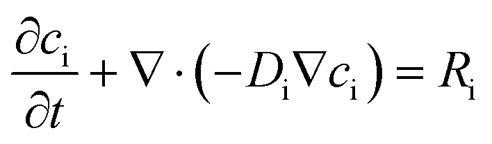 | (1) |
Generation of ions H+ and OH− (Rel) takes place at the anode (RH+,1) and cathode (ROH−,1) during each pulse (Eqn (2)), assuming a homogeneous profile over the surface of the electrodes.31
 | (2) |
Neutralization reaction occurs when protons meet hydroxides.

| Rneut = RH+,2 = ROH−,2 = −k1[H][OH] + k2 × 55.65 | (3) |
We consider one equilibrium between HPO42− and H2PO4−.
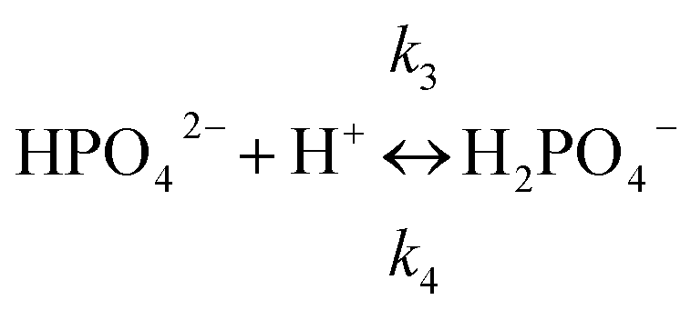
| Rbuf = RH+,3 = RHPO42−,3 = −RH2PO4−,3 = −k3[HPO42−][H+] + k4[H2PO4−] | (4) |
Acknowledgements
We thank NSF CBET 1016547 and NCI R21CA174577 for financial support of this research.References
- L. H. Silvertand, J. S. Torano, W. P. van Bennekom and G. J. de Jong, J. Chromatogr. A, 2008, 1204, 157–170 CrossRef CAS PubMed.
- K. Shimura, Electrophoresis, 2009, 30, 11–28 CrossRef CAS PubMed.
- J. Salplachta, A. Kubesova and M. Horka, Proteomics, 2012, 12, 2927–2936 CrossRef CAS PubMed.
- S. Hjerten, K. Elenbring, F. Kilar, J. L. Liao, A. J. Chen, C. J. Siebert and M. D. Zhu, J. Chromatogr., 1987, 403, 47–61 CrossRef CAS.
- U. Schnabel, F. Groiss, D. Blaas and E. Kenndler, Anal. Chem., 1996, 68, 4300–4303 CrossRef CAS.
- D. W. Armstrong, G. Schulte, J. M. Schneiderheinze and D. J. Westenberg, Anal. Chem., 1999, 71, 5465–5469 CrossRef CAS.
- M. Horka, J. Planeta, F. Ruzicka and K. Slais, Electrophoresis, 2003, 24, 1383–1390 CrossRef CAS PubMed.
- Y. Shen, S. J. Berger and R. D. Smith, Anal. Chem., 2000, 72, 4603–4607 CrossRef CAS.
- B. Alberts, Molecular biology of the cell, Garland Science, New York, 2002 Search PubMed.
- A. Varki, R. D. Cummings, J. D. Esko, H. H. Freeze, P. Stanley, C. R. Bertozzi and G. W. Hart, Essentials of Glycobiology, Cold Spring Harbor Laboratory Press, Cold Spring Harbor, NY, 2009 Search PubMed.
- G. M. Cook, Biol. Rev. Cambridge Philos. Soc., 1968, 43, 363–391 CrossRef CAS PubMed.
- T. Angata and A. Varki, Chem. Rev., 2002, 102, 439–469 CrossRef CAS PubMed.
- J. El-Ali, P. K. Sorger and K. F. Jensen, Nature, 2006, 442, 403–411 CrossRef CAS PubMed.
- N. Agrawal, Y. A. Hassan and V. M. Ugaz, Angew. Chem., Int. Ed., 2007, 46, 4316–4319 CrossRef CAS PubMed.
- P. G. Schiro, M. X. Zhao, J. S. Kuo, K. M. Koehler, D. E. Sabath and D. T. Chiu, Angew. Chem., Int. Ed., 2012, 51, 4618–4622 CrossRef CAS PubMed.
- C. D. K. Sloan, P. Nandi, T. H. Linz, J. V. Aldrich, K. L. Audus and S. M. Lunte, Annu. Rev. Anal. Chem., 2012, 5, 505–531 CrossRef CAS PubMed.
- L. Goodridge, C. Goodridge, J. Wu, M. Griffiths and J. Pawliszyn, Anal. Chem., 2003, 76, 48–52 CrossRef PubMed.
- M. Horká, F. Růžička, A. Kubesová, V. Holá and K. Šlais, Anal. Chem., 2009, 81, 3997–4004 CrossRef PubMed.
- M. Horká, F. Růžička, V. Holá, V. Kahle, D. Moravcová and K. Šlais, Anal. Chem., 2009, 81, 6897–6904 CrossRef PubMed.
- M. M. Martin and L. Lindqvist, J. Lumin., 1975, 10, 381–390 CrossRef CAS.
- D. Milanova, R. D. Chambers, S. S. Bahga and J. G. Santiago, Electrophoresis, 2011, 32, 3286–3294 CrossRef CAS PubMed.
- A. K. Vijh and B. E. Conway, Chem. Rev., 1967, 67, 623–664 CrossRef CAS.
- T. Geng, N. Bao, N. Sriranganathanw, L. Li and C. Lu, Anal. Chem., 2012, 84, 9632–9639 CAS.
- E. Prodan, C. Prodan and J. H. Miller, Biophys. J., 2008, 95, 4174–4182 CrossRef CAS PubMed.
- H. Y. Wang and C. Lu, Anal. Chem., 2006, 78, 5158–5164 CrossRef CAS PubMed.
- N. Bao, J. Wang and C. Lu, Electrophoresis, 2008, 29, 2939–2944 CAS.
- M. A. Unger, H. P. Chou, T. Thorsen, A. Scherer and S. R. Quake, Science, 2000, 288, 113–116 CrossRef CAS.
- Z. Cao, F. Chen, N. Bao, H. He, P. Xu, S. Jana, S. Jung, H. Lian and C. Lu, Lab Chip, 2013, 13, 171–178 RSC.
- J. Schindelin, I. Arganda-Carreras, E. Frise, V. Kaynig, M. Longair, T. Pietzsch, S. Preibisch, C. Rueden, S. Saalfeld, B. Schmid, J. Y. Tinevez, D. J. White, V. Hartenstein, K. Eliceiri, P. Tomancak and A. Cardona, Nat. Methods, 2012, 9, 676–682 CrossRef CAS PubMed.
- W. M. Haynes, CRC Handbook of Chemistry and Physics, Taylor and Francis Group, 2010 Search PubMed.
- D. Di Carlo, C. Ionescu-Zanetti, Y. Zhang, P. Hung and L. P. Lee, Lab Chip, 2005, 5, 171–178 RSC.
Footnote |
| † Electronic supplementary information (ESI) available: Figures S1–S5 and videos S1–S2. See DOI: 10.1039/c4sc00319e |
| This journal is © The Royal Society of Chemistry 2014 |