
 Open Access Article
 This Open Access Article is licensed under a
 Creative Commons Attribution 3.0 Unported Licence
Voronoi polyhedra probing of hydrated OH radical†
Lukasz Kazmierczak and
Dorota Swiatla-Wojcik*
Institute of Applied Radiation Chemistry, the Faculty of Chemistry, Lodz University of Technology, Zeromskiego 116, 90-924 Lodz, Poland. E-mail: swiatlad@p.lodz.pl
First published on 28th August 2014
Abstract
We present 3D-characterization of the solvated ˙OH radical in water at 37 °C using the Voronoi polyhedron technique. Assuming that the ˙OH solvation cage is represented by the minimal-volume polyhedron we have calculated statistical distributions of the metric and topological properties of the solvation cage. The statistical means 10.1, 3.26 Å, 27.2 Å3, and 1.50, have been obtained for the solvation number, the face-weighted cage-radius, the free volume of ˙OHaq, and the asphericity factor, respectively. The mean value of the face-weighted radius coincides with the maximum of the radical-water radial distribution function. Similar properties of the polyhedra constructed for the hydrogen bonded radical and for the unbound one confirm the mechanistic view of the localization of ˙OH in cavities in the hydrogen-bond network. The distribution of the asphericity factor reveals the existence of ice-like regions. A short review of the graphical software used for 3D-visualization includes MS Excel, Maple, and POV-Ray programs. A practical user guide is provided in the ESI.†
Introduction
Insight into a solvation cage (shell) of a solute provided by classical molecular dynamics (MD) and Monte Carlo (MC) simulations or by DFT-based Car–Parrinello Molecular Dynamics (CPMD) requires computational tools for visualization and statistical description of the simulated structures.1,2 The simplest and commonly used tool is a partial radial distribution function (RDF). RDF describes site–site solute–solvent correlation in space.1 A serious drawback resulting from the one-dimensional nature of a RDF is that 3D correlations are averaged out. Although more thorough insight can be provided by using angular-dependent pair distribution or spatial distribution functions,3,4 construction of the Voronoi polyhedron (VP) offers a unique qualitative tool for 3D-characteristics of the nearest neighbourhood of a solute.5 The Voronoi polyhedron associated with a given point (atom) is defined as the convex region of space closer to this point than to any other points (atoms). Mathematically VP follows a concept embodied in a Wigner–Seitz primitive cell in crystallography.6 Metric and topological properties of VP quantify the space owned by a solute in a solution. These properties may be used to describe size and shape of a solvation cage (shell) providing estimates for the free volume and the number of neighbouring solvent molecules (the solvation number).In the present paper we employ a method of VP construction to provide the first comprehensive statistical description of the metric and topological properties of the hydrated hydroxyl radical (˙OHaq). The problem of ˙OH solvation in aqueous media is important because of its relevance to atmospheric chemistry, biology, medicine, radiobiology, and radiation chemistry. Hydroxyl radicals are highly reactive and consequently short-lived. In biological systems, ˙OH radicals produced from the decomposition of hydro-peroxides, cause much cell damage.7,8 Hydroxyl radicals generated in the troposphere remove volatile organic compounds (VOCs) and methane from the air.9 In aqueous systems exposed to ionizing radiation ˙OH is the main oxidant formed.10 Taking into account a key role of the hydroxyl radical in biology and medicine we have recently carried out classical MD simulation for a diluted aqueous solution of ˙OH at the body temperature (37 °C).11 Using partial RDFs calculated for the solute–solvent and solvent–solvent sites we showed that ˙OH radical is coordinated by 13–14 solvent molecules and tends to occupy cavities in the hydrogen-bond (HB) network of water. Liquid water at 37 °C resembles a gel-like HB network, where rotations cause individual hydrogen bonds to break and quickly re-form in new configurations.12 The localization in cavities is thus consistent with a small number of hydrogen bonds established by ˙OH. According to the geometrical definition of hydrogen bond, ˙OH radical was not hydrogen-bonded in ca. 30% of cavities.11 In other cases, ˙OH formed mostly one hydrogen-bond to the surrounding water molecules, usually acting as a proton-donating partner (H-donor). Compared to neat water the continuous lifetime of H-donor bond (0.033 ps) was an order of magnitude smaller, but the intermittent lifetime of a few picoseconds was similar.13 Our later study showed that although the mean number of water–water hydrogen bonds is the same in solution and in neat water, the HB connectivity pattern of solvent molecules is different.14 Namely, in the presence of ˙OH ice-like patches, i.e. supramolecular structures of continuously connected four-bonded molecules, are noticeably smaller.
To develop our mechanistic view on localization of ˙OH in aqueous media we have elaborated a VP-based approach and processed a molecular dynamics simulation trajectory to calculate metric and topological properties of the molecular neighbourhood of ˙OHaq. At the same time properties of the constructed VPs characterize cavities in the HB network occupied by the hydroxyl radical. To provide the 3D-visualization we use graphical facilities of commercial MS Excel spreadsheet application, Maple computer algebra system, and freeware POV-Ray (Persistence of Vision Raytracer) ray-tracing program. Advantages and drawbacks of these visualization methods are shortly discussed. Technical and mathematical details are given in ESI.†
Methodology and results
A problem of VP construction has been formulated with respect to the oxygen atoms, nearly allocating mass centres of the ˙OH and H2O molecules. The oxygen atom of ˙OH is taken as the central point (centre) about which the Voronoi polyhedron is constructed. By definition, VP is the minimal polyhedron whose planar faces are perpendicular bisector planes of lines joining the centre to the oxygen atoms of the neighbouring H2O molecules. A region delimited by so determined polyhedron unambiguously defines the space owned by the radical in solution. Since there is one face for each of the nearest neighbours, the number of faces specifies the coordination (solvation) number.To calculate the topological and metric properties of ˙OHaq we have processed the MD simulation trajectory obtained previously.11 The simulation was carried out for the system containing 400 water molecules and one radical molecule at the density 0.994 g cm−3, corresponding to the density of neat water at 37 °C. Radical and water molecules were described by the flexible models two-site11 and three-site,15 respectively. The employed model potentials include short-range pair interactions of hydrogen atoms to better describe spatial hindrance resulting from the presence of HB network. The simulation time step of 0.1 fs was assumed. The stability of the total energy was 10−6 < ΔE/E < 10−5. After the equilibration stage of about 40 ps, the simulation was extended up to 30 ps. The average temperature of the run was 313 ± 6 K. The equilibrium configurations were recorded every tenth simulation step. We have analyzed 2.5 × 10⁴ equilibrium configurations. The algorithm designed to construct VP is described below. Mathematical details can be found in ESI.†
Construction of Voronoi polyhedron
For a given configuration we have selected coordinates of water oxygen atoms (Oi = 1,2,…,N) within an initially chosen spherical neighbourhood of the radical oxygen atom (central point C) and determined N perpendicular bisector planes to lines joining C with each of the Oi atoms. For each plane we marked the region shared with point C. An intersection point of three planes located on the same side of the individual plane as the point C has been classified as VP vertex. To determine edges and faces vertices belonging to each bisector plain have been sorted and correspondingly numbered. Details of sorting method are given in ESI.†For any convex polyhedron the numbers of faces (NF), edges (NE), and vertices (NV) are related by Euler relationship:
| NF + NV − NE = 2 | (1) |
Since each vertex is the intersection of three bisector planes, NE and NV are related by NE = 3/2 NV, and the topological condition, eqn (1), can be written as:
| NV − 2NF + 4 = 0 | (2) |
Calculation of metric properties
Using the coordinates of the numbered vertices we calculate a surface area of each face Si (i = 1, 2,…, NF):
 | (3) |
In eqn (3) index 1i corresponds to the vertex #1 belonging to the i-th face and Mi denotes the intersection point of COi line and the i-th bisector plane.
The volume of VP can be calculated as:
 | (4) |
Taking the tabulation step of 0.01 Å we have varied the neighbourhood radius from 2.5 to 6 Å. The topological condition eqn (2) has not been satisfied for the radius smaller than 3.26 Å. Fig. 1 shows how the VP volume (Vol) and the number of faces (NF) change with the increasing neighbourhood radius. Whilst NF increases Vol rapidly decreases approaching the lowest level at a certain radius R marked in the figure. Polyhedra constructed for higher radius are less sharp because of newly-built small faces corresponding to more distant solvent molecules. Appearance of these faces does not change the volume. Polyhedron that corresponds to the radius R has been identified with the solvation cage of ˙OH. Consequently, the number of faces NF (R) has been taken as the solvation (coordination) number of ˙OHaq. Metric and topological properties have been calculated for the minimal-volume VP with the smallest number of faces.
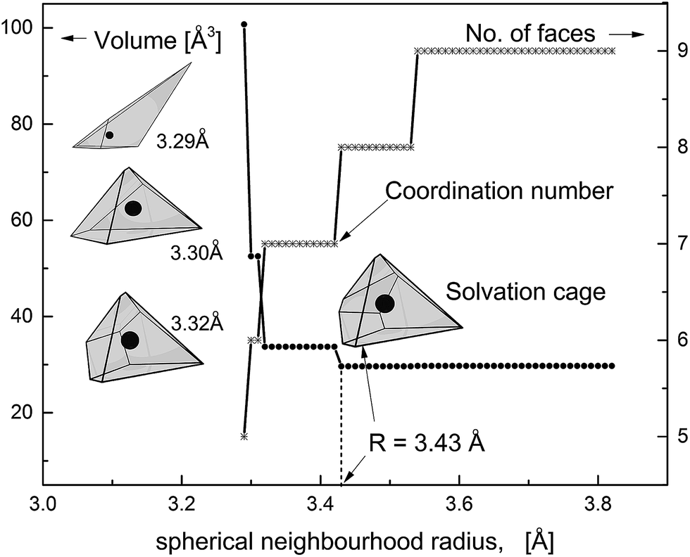 | ||
| Fig. 1 Volume (left axis) and the number of faces (right axis) of VP constructed for the water oxygen atoms within a varying spherical neighbourhood. The constructed VP is visualized for the selected radii (3.29, 3.30, 3.32, and 3.43 Å). The solvation cage is represented by the minimal-volume VP with the smallest number of faces (the coordination number). | ||
Calculation of topological properties
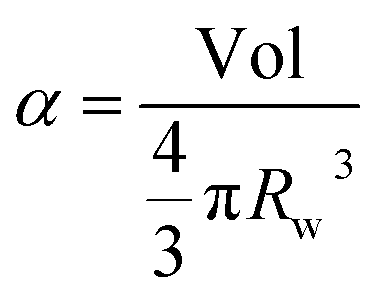
Apart from the cage-radius (R) we define the face-weighted radius (Rw) as:
 | (5) |
In eqn (5) the contribution of molecules providing larger faces is enhanced by the weighting factor. Taking eqn (4) Rw can be alternatively expressed as:
 | (6) |
So defined face-weighted radius is related with asphericity factor (α) commonly expressed as:16,17
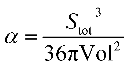 | (7) |
From eqn (6) and (7) we obtain:
 | (8) |
In order to improve a description of the topological properties we have also defined volume quotient Qvol, and distance quotient Qdist. Namely, for a given VP we have set vertex Omax which is the most distant from the centre C and plane Π perpendicular to the vector  . Plane Π divides VP into part A of volume VA, comprising Omax, and part B of volume VB = Vol − VA. Quotients Qvol and Qdist have been expressed as:
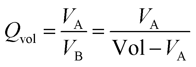 | (9) |
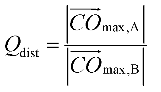 | (10) |
In eqn (10) Omax,B denotes the most distant vertex in part B.
Visualization
3D-presentation of VP is essential for both verification of the implemented computational procedure and visualization of a solvation cage. We have tested three visualization methods using computational tools provided by Microsoft Excel spreadsheet application, Maple computer algebra system, and Persistence of Vision Raytracer (POV-Ray) program. The two former are commercial software, whereas POV-Ray is a freeware program. Advantages and drawbacks of the tested methods are shortly discussed below. Sample imagines are depicted in Fig. 2.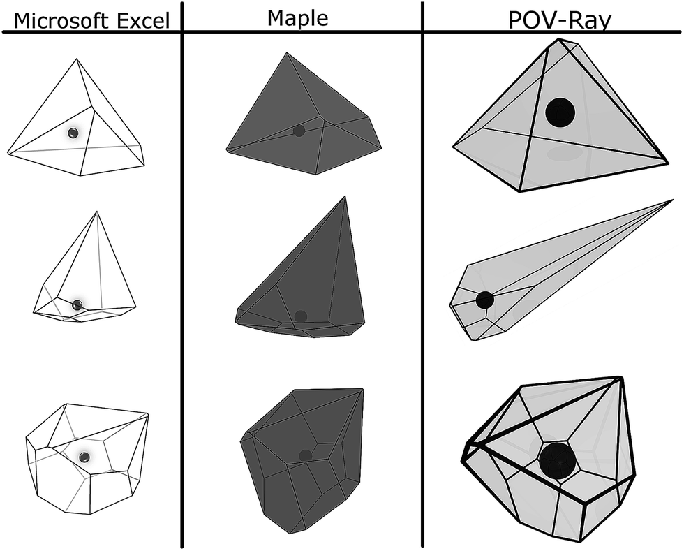 | ||
| Fig. 2 Three-dimensional imagines of ˙OH solvation cage created by Microsoft Excel, Maple, and POV-Ray. The position of ˙OH is marked by a central dot. | ||
Input data for all the methods tested are the coordinates of sorted vertices belonging to each of the VP faces. Three-dimensional presentation of a solvation cage by using the spreadsheet application is not straightforward. The user has to implement orthogonal projections applying the Gram–Schmidt process.18 The Maple software offers a command-line utility and ready-to-use macros accepting basic graphical options (colour, transparency, line-style, etc.). It makes 3D-visualization of a solvation cage rather intuitive and easy. POV-Ray program creates photo-realistic images using an advanced rendering technique, called ray-tracing. The POV-Ray code is written in object-oriented C++, hence handling may be difficult for users less familiar with programming languages. Technical and mathematical details on three visualization methods are provided in ESI.†
Statistical handling of VP properties
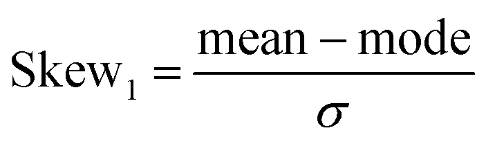
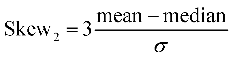
Calculated probability distributions (normalized probability density functions) of the metric and topological properties of ˙OH solvation cage are displayed in Fig. 3–5. Statistical description of these distributions is presented in Table 1. We have calculated mean, standard deviation (σ), median, mode, and four dimensionless parameters: Skew1 (eqn (11)), Skew2 (eqn (12)), asymmetry coefficient γ (eqn (13)), and Kurtosis (eqn (14)). Skew1 and Skew2, describe to what extent a given distribution function leans of its mean.
 | (11) |
 | (12) |
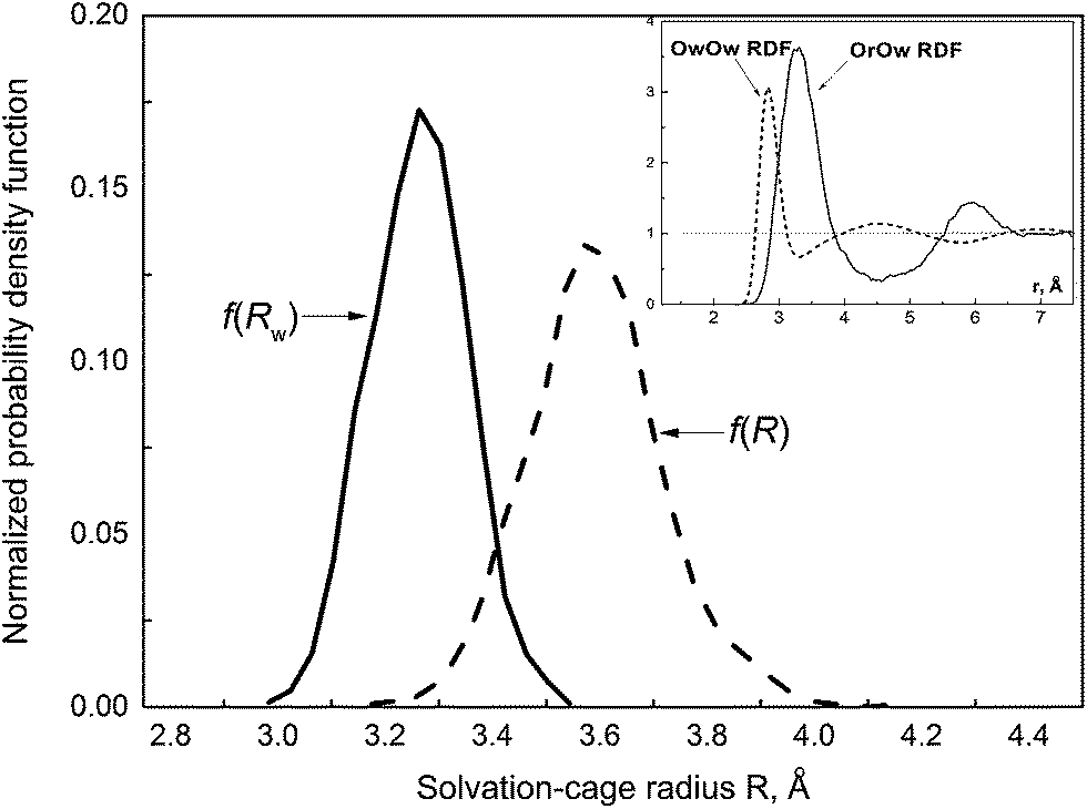 | ||
| Fig. 3 The normalized probability distribution function of the cage-radius R and the face-weighted radius Rw. Inset shows the OrOw RDF (solid)11 and the OwOw RDF (dash) obtained from the MD simulation of neat water at 37 °C.12 | ||
| R [Å] | Rw [Å] | Vol [Å3] | NF | Stot [Å2] | Qvol | Qdis | α | |
|---|---|---|---|---|---|---|---|---|
| a See text for definitions. | ||||||||
| Mean | 3.59 | 3.26 | 27.24 | 10.10 | 50.07 | 1.16 | 1.32 | 1.50 |
| Standard deviation σ | 0.13 | 0.09 | 3.70 | 1.08 | 6.40 | 0.33 | 0.38 | 0.20 |
| Median | 3.59 | 3.26 | 26.64 | 10.12 | 48.81 | 1.10 | 1.20 | 1.46 |
| Mode | 3.584 | 3.272 | 26.32 | 10.15 | 47.29 | 1.05 | 1.05 | 1.41 |
| Dimensionless parameters | ||||||||
| Skew1 | 0.05 | −0.13 | 0.25 | −0.05 | 0.43 | 0.33 | 0.71 | 0.45 |
| Skew2 | 0.00 | 0.00 | 0.48 | −0.06 | 0.59 | 0.55 | 0.95 | 0.60 |
| Asymmetry coefficient γ | 0.230 | 0.00 | 2.44 | −0.23 | 2.81 | 3.12 | 3.72 | 3.00 |
| Kurtosis | 3.42 | 2.83 | 15.4 | 3.00 | 18.3 | 22.7 | 25.7 | 21.1 |
For a perfectly symmetric unimodal distribution, mean = median = mode, and the skewness parameters are equal to zero.
The asymmetry coefficient γ is defined as the third standardized moment of a given distribution function:
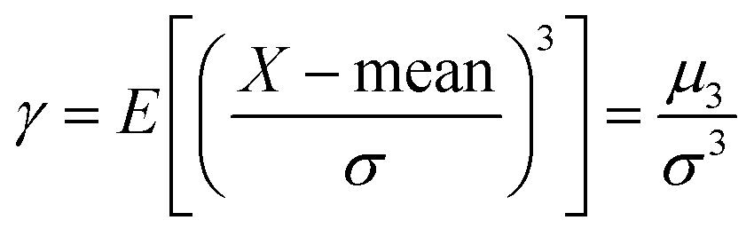 | (13) |
In eqn (13) E and μ3 denote the expectation operator and the 3rd central moment, respectively.
Kurtosis is defined as the fourth standardized moment. It is a measure of the “peakedness” of a distribution and the “heaviness” of its shoulders.
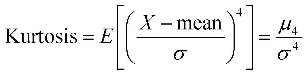 | (14) |
For the normal distribution Kurtosis = 3.
Discussion
RDF versus VP method
Solute–solvent partial RDFs are commonly used to assess the size of a solvation cage and the coordination (solvation) number. Regarding the size, both the maximum and the minimum of the first peak are considered, whereas the solvation number is defined as a running integration number spanning the first peak:
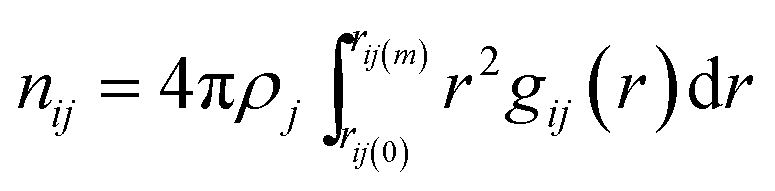 | (15) |
In eqn (15) ρj is the number density of the j-th site, gij is the partial RDF calculated for sites i and j, rij(0) and rij(m) delimit the position of the first peak. The nearest neighbourhood of ˙OH is described by a set of four partial RDFs, OrOw, OrHw, HrOw, HrHw, where the subscripts r and w refer to the radical and water molecules. Features of the calculated RDFs are listed in Table 2. Taking the values of rij(m) one may assess a size of the solvation cage as about 4.5 Å. This estimate is well above the mean cage-radius R (see Table 1). Although the probability density function f(R), displayed in Fig. 3, shows slightly positive skew, the right-hand tail extends up to 4.2 Å, i.e. noticeably below rij(m). It indicates that the position of the first minimum substantially overestimates the size of ˙OH solvation cage. Compared to f(R) the probability distribution of the face-weighted radius Rw, also depicted in Fig. 3, is more compact, noticeably shifted to the left, and shows the negative Skew1. These differences suggest some asymmetry of ˙OH solvation cage discussed in the next section. As shown in the inset, the mean value of Rw (3.26 Å) coincides with the maximum position of the OrOw RDF. At the same time it coincides with the first minimum of the OwOw RDF calculated from the simulation of pure water at 37 °C.12
| Feature/sites(ij) | OrOw | OrHw | HrOw | HrHw |
|---|---|---|---|---|
| rij(max) | 3.25 ± 0.07 | 2.82 ± 0.03 | 3.15 ± 0.05 | 3.03 ± 0.05 |
| rij(min) | 4.49 ± 0.08 | 4.41 ± 0.08 | 4.76 ± 0.09 | 4.51 ± 0.08 |
| nij | 14.1 ± 0.4 | 25.7 ± 0.9 | 15.4 ± 1.0 | 26.1 ± 1.1 |
Accuracy of partial coordination number nij listed in Table 2 depends on a quality of the respective RDF. If the first minimum is broad and poorly defined nij is subjected to a significant uncertainty. The coordination numbers nOrOw nOrHw nHrOw nHrHw indicate that the solvation cage of ˙OH comprises 13–14 water molecules. The VP-based approach provides a statistical distribution of the number of faces NF, identified with the solvation number. The probability density function f(NF) displayed in Fig. 4 is not Gaussian, although its kurtosis is near 3. A small negative skewness is indicated by Skew1, Skew2 parameters, and asymmetry coefficient γ. The mean value (10.10) and the standard deviation (1.08) of f(NF) show that the typical solvation cage contains 9, 10, or 11 water molecules. As shown in the inset mean NF is reproduced by the OrOw running integration number at about 3.6 Å, corresponding to the mean value of cage-radius R. If, in turn, the mean value of face-weighted radius Rw (3.26 Å) is substituted for the upper integration limit in eqn (15), the running integration number gives 4.5. This value coincides with the nOwOw coordination number extracted from the simulation of neat water at 37 °C.12 Thus the spherical neighbourhood delimited by Rw comprises closer located solvent molecules in the number characteristic for the structural properties of liquid water. It may suggest that ˙OH occupying deformations in the hydrogen-bond network takes place of H2O molecules.
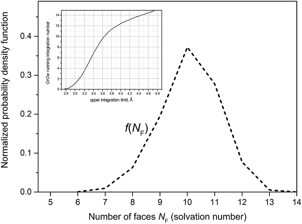 | ||
| Fig. 4 Probability distribution of the ˙OH coordination number, i.e. the number of faces NF. Inset shows the OrOw running integration number versus the upper integration limit in eqn (15). | ||
To summarise this section, the conventional methods based on RDFs overestimate both the solvation number and the size of the solvation cage. Regarding the latter, the position of the RDF maximum seems to be more reliable estimate.
Metric and topological properties
Metric and topological properties are not available in the conventional analysis based on RDFs. These properties can be easily captured using the developed methodology. Fig. 5 presents the probability distribution of the metric properties of solvation cage: the volume (Vol) and the total number of faces (Stot). Both f(Vol) and f(Stot) are highly leptokurtic (Kurtosis > 3) and show noticeable positive skewness. The mean = 27.24 Å3 provides an estimate for the free volume of ˙OH in aqueous solution. This cage capacity is reproduced by a sphere of radius 1.87 Å that is much smaller compared to mean R or Rw. It may suggest asphericity or shape irregularity of solvation cage. To verify our supposition we have calculated the probability distributions of spatial anisotropy parameters (α, Qvol, Qdist). The distribution of the asphericity factor α ranges from 1.2 to 2.3 and shows mean = 1.50, median = 1.46, mode = 1.41, and highly positive asymmetry coefficient γ. The calculated mode is close to the asphericity factor of a rhombic dodecahedron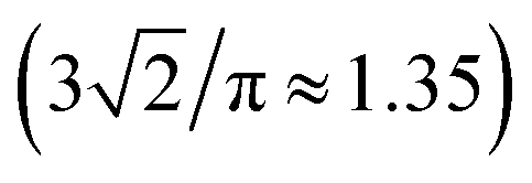 , whereas mean is close to α = 1.58 obtained for the local environment of H2O molecules in ambient water.17 It was previously believed that the radical predominantly occupies distortions in the HB network.11,14 However, we have found that ca. 5% of solvation cages shows the asphericity comparable with the Wigner–Seitz cell of the Ih ice lattice (αIh = 2.25). This result indicates that ˙OH is also located in ice-like regions (patches). At the same time it confirms the existence of patches in neat water12 and in the diluted solution14 at 37 °C. Since noticeably smaller patches were found in solution14 one may conclude that localization of ˙OH in patches perturbs the connectivity of four-bonded water molecules.
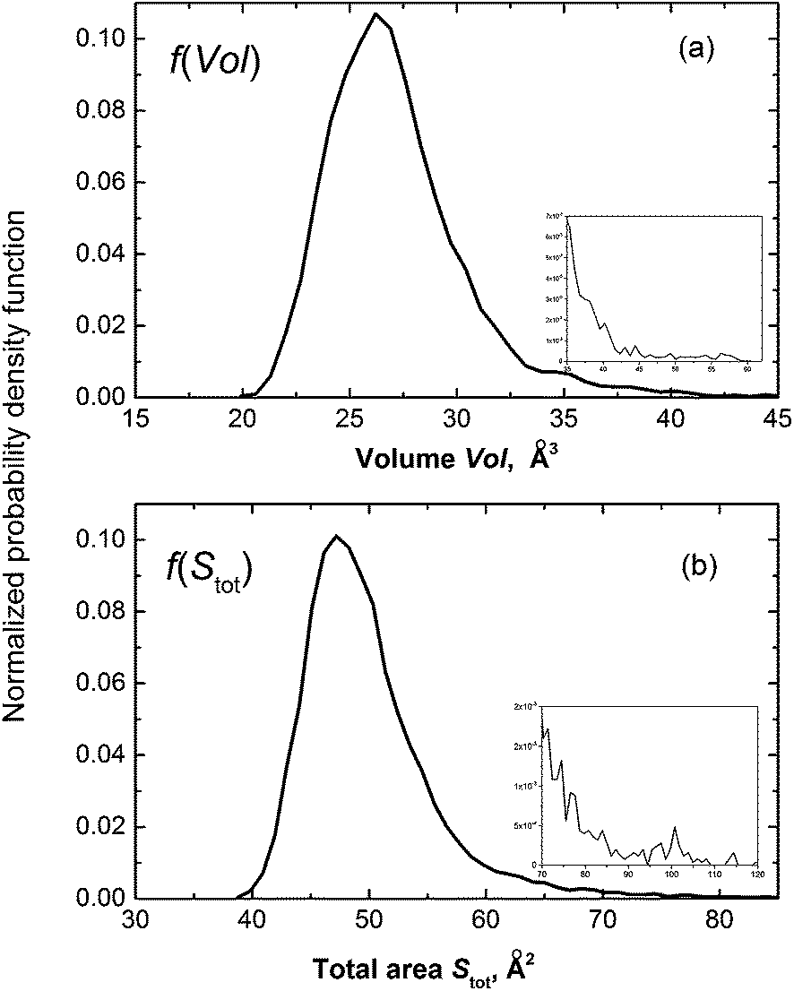 | ||
| Fig. 5 Probability distribution of the metric properties: (a) VP volume Vol; and (b) total area of faces Stot. | ||
Shape irregularity of the solvation cage is characterized by Qvol and Qdist. Some of the constructed VPs show distinct disproportion of faces making an impression of shape sharpening (cf. Fig. 2). Such irregularity indicates close proximity of some neighbours and compaction of the others at the opposite side of the radical. As defined by eqn (9), Qvol presents a volumetric ratio of the sharp and the more regular parts of the solvation cage, whereas Qdist in eqn (10) describes an axial asymmetry of these two parts. The probability distributions calculated for Qvol and Qdist show mean and median close to unity, but both are highly leptokurtic. For about one-fifth of cages Qvol and Qdist exceeded 1.5. In Fig. 6 the anisotropy parameters (α, Qvol, Qdist) are presented as a function of the solvation number NF. As it can be seen, higher coordination numbers correspond to less aspherical and less anisotropic cages. We have found that for NF > 12 the volume quotient Qvol is less than unity. It means that the compact part of ˙OH cage takes a larger volume than the sharper one.
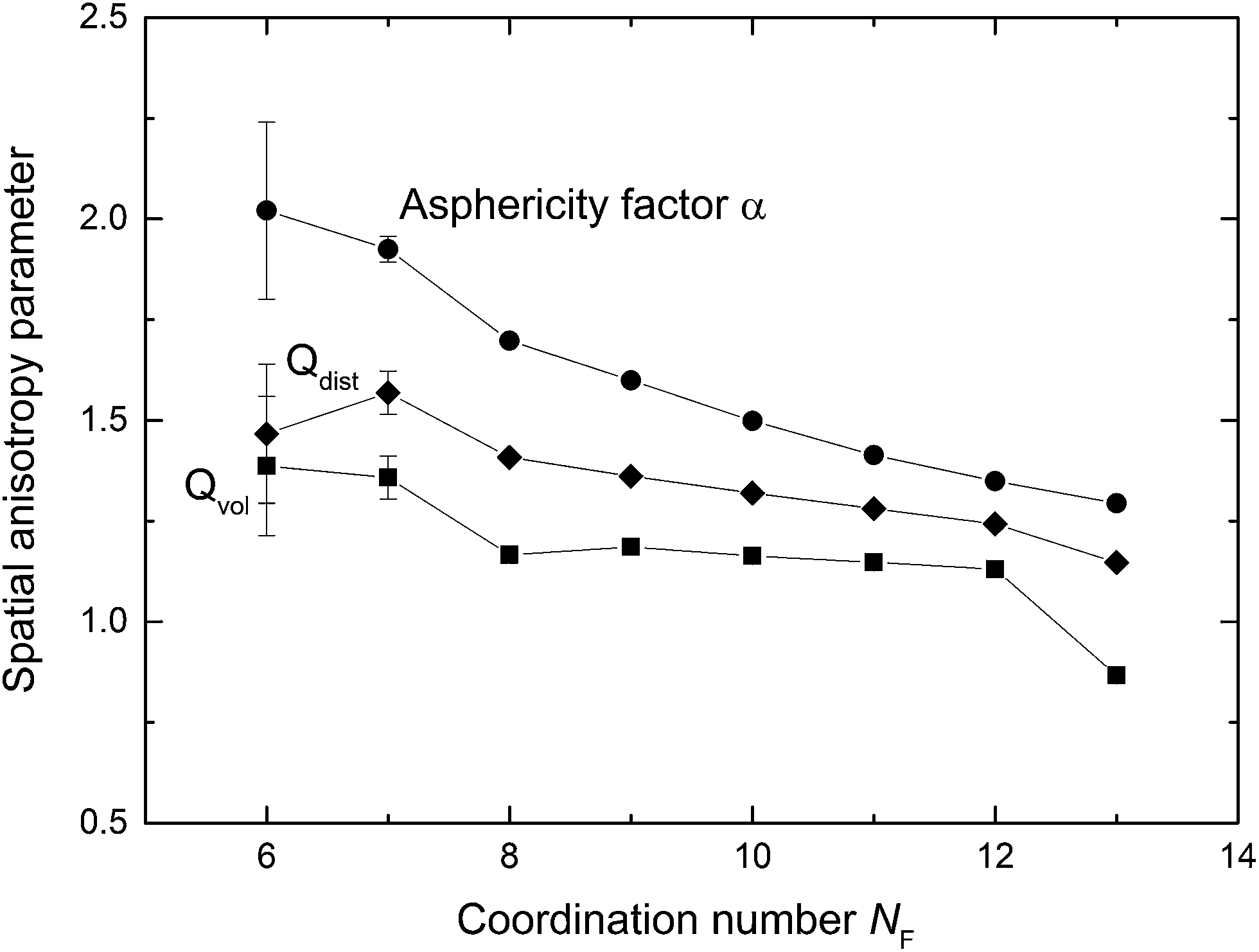 | ||
| Fig. 6 Spatial anisotropy parameters versus the ˙OH solvation number (the number of faces NF): the asphericity factor α (circles), the volume quotient Qvol (squares), and the distance quotient Qdist (diamonds). | ||
Hydrogen bonding issue
Water is a highly associated liquid. Extensive assembling of molecules via hydrogen bonds controls most of the solvent properties of water. Solvation may be considered as a compromise between water–water and solute–water interactions, minimizing Gibbs free energy of the system. Although the Voronoi polyhedra are constructed on the basis of the oxygen atoms, the hydrogen bonding problem can be addressed. We have compared the properties of VP constructed for the hydrogen bonded ˙OH radical and for the unbound one. To distinguish these two species we have followed the extended energetic definition of H-bond, used previously.11,14 According to this definition a pair of the molecules is hydrogen bonded if a distance between the hydrogen atom of the H-donating partner and the oxygen atom of the H-acceptor is less than 2.5 Å, an angle between the O–H bond of the H-donor and the line connecting the oxygen atoms is not larger than 30°, and the pair interaction energy is at least equal to −8 kJ mol−1.The shape of the VP constructed the H-bonded ˙OH have been analysed for 2 × 10³ configurations. Analysis of the molecular neighbourhood of the unbound radical has been performed for 2 × 10⁴ configurations. The statistical parameters of the distributions of metric and topological properties calculated for the H-bonded ˙OH and for the unbound radical differ by less than 2%. We have found that the asphericity factor α obtained for the solvation cage of the H-bonded ˙OH is slightly higher, whereas the mean and mode of distribution of other properties (R, Rw, NF Vol, Stot, Qvol and Qdist) are slightly lower. Such a small difference between the H-bonded and the unbound ˙OH can be expected assuming the cavity mechanism of localization.11,14 Given that, the constructed VPs reveal the shape of cavities of the HB network.
Summary and conclusion
In this paper we report an analysis of the hydrated ˙OH using computational techniques based on Voronoi polyhedra to process MD simulation trajectory. Construction of Voronoi polyhedra offers a qualitative tool for 3D-characterization of the molecular neighbourhood. Assuming that the solvation cage of ˙OH is represented by the minimal-volume Voronoi polyhedron (constructed around the radical oxygen atom) we have calculated the statistical distribution of the metric and topological properties of ˙OHaq at the biologically important temperature (37 °C). Our calculations show that the conventional methods based on RDFs overestimate both the solvation number and the size of the solvation cage. The statistical mean of the number of faces of VP indicates that ˙OH is coordinated by 10 water molecules. This number is noticeably smaller compared to the solvation number (13–14) resulting from the analysis based on partial RDFs. Metric and topological properties of the constructed Voronoi polyhedra reveal features that cannot be captured by RDFs. The most important results that improve understanding of the solvation of ˙OH in water are listed below. (1) We have found that smaller solvation numbers correspond to more aspherical and more anisotropic solvation cages. (2) The face-weighted radius (3.26 Å) delimits the neighbourhood of closer located solvent molecules in the number characteristic for the structural properties of liquid water. (3) The mean volume of Voronoi polyhedra (27.2 Å3) provides an estimate for the free volume of ˙OHaq. (4) The distribution of the asphericity factor reveals the existence of ice-like regions. (5) The Voronoi polyhedra constructed for the H-bonded ˙OH and for the unbound radical show very similar properties as it can be expected assuming localization of ˙OH in cavities in HB network.References
- C. J. Cramer, Essentials of Computational Chemistry: Theories and Models, Wiley, New York, 2nd edn, 2004 Search PubMed.
- R. Iftimie, P. Minary and M. E. Tuckerman, Proc. Natl. Acad. Sci., 2005, 19, 6654 CrossRef PubMed.
- C. Oldiges, K. Wittier, T. Tönsing and A. Alijah, J. Phys. Chem. A, 2002, 106, 7147 CrossRef CAS.
- J. M. Khalack and A. P. Lyubartsev, J. Phys. Chem. A, 2005, 109, 378 CrossRef CAS PubMed.
- E. E. David and C. W. David, J. Chem. Phys., 1982, 76, 4611 CrossRef CAS PubMed.
- M. O'Keefe, Acta Crystallogr., Sect. A: Cryst. Phys., Diffr., Theor. Gen. Crystallogr., 1979, 35, 772 CrossRef.
- B. Halliwell and J. H. C. Gutteridge, Free Radicals in Biology and Medicine, Oxford University Press, Oxford, UK, 3rd edn, 1999 Search PubMed.
- W. Stumm and J. J. Morgan, Aquatic Chemistry, Wiley, New York, 1996 Search PubMed.
- J. H. Seinfeld and S. N. Pandis, Atmospheric Chemistry and Physics: from Air Pollution to Climate Change, John Wiley & Sons, Inc., New York, 1998 Search PubMed.
- G. V. Buxton, in Charged Particles and Photon Interactions with Matter, ed. A. Mozumder and Y.Hatano, Marcel Dekker, New York, Basel, 2004, p. 331 Search PubMed.
- A. Pabis, J. Szala-Bilnik and D. Swiatla-Wojcik, Phys. Chem. Chem. Phys., 2011, 13, 9458 RSC.
- D. Swiatla-Wojcik and J. Szala-Bilnik, J. Chem. Phys., 2011, 134, 054121 CrossRef PubMed.
- D. Swiatla-Wojcik, Chem. Phys., 2007, 342, 260 CrossRef CAS PubMed.
- D. Swiatla-Wojcik and J. Szala-Bilnik, J. Chem. Phys., 2012, 136, 064510 CrossRef PubMed.
- P. Bopp, G. Jancso and K. Heinzinger, Chem. Phys. Lett., 1983, 98, 129 CrossRef CAS.
- G. Ruocco, M. Sampoli and R. Vallauri, J. Chem. Phys., 1992, 96, 6167 CrossRef CAS PubMed.
- P. Jedlovszky, J. Chem. Phys., 1999, 111, 5975 CrossRef CAS PubMed.
- W. H. Greub, Linear Algebra, Springer-Verlag, New York, 4th edn, 1975, p. 226 Search PubMed.
Footnote |
| † Electronic supplementary information (ESI) available. See DOI: 10.1039/c4ra04181j |
| This journal is © The Royal Society of Chemistry 2014 |