A FRET analysis of dye diffusion in core/shell polymer nanoparticles†
Luis Cerdán*a,
Eduardo Encisob,
Leire Gartzia-Riveroc,
Jorge Bañuelosc,
Iñigo López Arbeloac,
Ángel Costelaa and
Inmaculada García-Morenoa
aInstituto de Química-Física “Rocasolano”, Consejo Superior de Investigaciones Científicas (CSIC), Serrano 119, 28006 Madrid, Spain. E-mail: lcerdan@iqfr.csic.es
bDepartamento de Química Física I, Facultad de Ciencias Químicas, Universidad Complutense de Madrid, Ciudad Universitaria, 28040 Madrid, Spain
cDepartamento de Química Física, Universidad del País Vasco-EHU, Aptdo. 644, 48080 Bilbao, Spain
First published on 1st May 2014
Abstract
In this paper we show that dye distributions within polymer core/shell nanoparticles (NPs), grown in multiple steps, are controlled not only by the synthesis route, but are also governed by dye diffusion between core and shell, resulting in dye distributions completely different from the targeted ones. We show that Förster Resonance Energy Transfer (FRET) dynamics can be used as a spectroscopic measure to determine the particular dye profiles along the NPs and thus to uncover the presence of dye diffusion. Finally, to confirm the previous results and with the aim to have a clearer understanding of the diffusion processes within core/shell NPs (equilibrium and transient dye distributions, time scales, etcetera), we analyze the behaviour predicted by existing diffusion models and infer that the dye diffusion is already finished at the end of the shell growth.
Introduction
Colloidal nanoparticles (NPs) are at the forefront of fundamental nanoscience, applied nanotechnology, biophotonics and nanomedicine thanks to their versatility, simplicity in manufacture, and, most importantly, due to the possibility of fine tuning their physical, optical and reactive properties in a controlled way.1–3 In particular, core/shell NPs are being extensively used in sensing and diagnosis applications due to the possibility of obtaining multifunctional systems in which core and shell present different functionalities (catalytic, plasmonic, magnetic, imaging, drug delivery).1,2,4,5 Although organic and inorganic compounds can be used and combined into a single core/shell NP,5 full organic core/shell NPs are of special interest for in vitro and in vivo biophotonic and nanomedicine applications due to their biocompatibility, drug delivery capabilities and post treatment biodegradation properties.In vivo and in vitro bioimaging techniques require of fluorescent probes with high brightness, high resistance to photodegradation, low toxicity and high water solubility.6 Probes fulfilling all of these properties are scarce, but this limitation can be circumvented by using highly efficient and photostable probes embedded into NPs, which provides water solubility, reduced cytotoxicity, and selective tissue targeting through surface functionalization.7 In addition, the fluorescence probes must emit in the red spectral region (>600 nm), as these wavelengths allow for deep tissue penetration and reduced interference with the background autofluorescence of biological samples. In this sense, Förster Resonance Energy Transfer (FRET), which is a physical process in which an excited donor transfers its energy to a nearby acceptor by means of dipole moments coupling,8 allows for obtaining highly efficient red emitting probes while exciting at the blue or green spectral region. The FRET efficiency is highly dependent, among other parameters, on the particular donor–acceptor mutual distance distribution, so that when dealing with FRET-based multifunctional core/shell NPs, the location where FRET is taking place (core, shell, or both) must be accurately controlled, and the implications of the particular distribution choice clearly understood.
We have recently developed a series of dye doped latex NPs based on acrylic monomers, with sizes ranging from 20 to 350 nm in diameter, exhibiting outstanding laser performances when using one9,10 or two laser dyes11 as dopants for the NPs in colloidal solutions, as well as controllable random laser emission in dried self-assembled monoliths.12 Given the control on the synthesis procedure attained with these NPs, they might serve as an appropriate test bed to prove the effects of the particular donor and acceptor distributions on the FRET efficiency and photophysics.
In this paper we evaluate the FRET process from Rhodamine 6G (Rh6G) to Nile Blue (NB), dyes with a very good spectral overlap,11 in core/shell NPs composed of dissimilar mixtures of methacrylic monomers and grown in multiple steps. First, we experimentally verify whether the synthesized NPs are indeed core/shell or if new NPs are nucleated as a consequence of the multistep growing. Then, we compare the FRET efficiency of two different NPs with the same size and donor and acceptor concentrations (in terms of number of molecules within each NP), but with diametrically different dye distribution (homogeneous vs. Rh6G in core/NB in shell). We make use of the FRET dynamics as a spectroscopic ruler to determine the particular dye profiles along the NPs and thus to uncover the presence of dye diffusion in the core/shell NPs. Finally, we evaluate theoretically the diffusion process in order to confirm the experimental results and gather the time scales involved.
Experimental and theoretical methods
Materials
Laser dyes Rhodamine 6G (Rh6G) (Fluka, >95% purity) and Nile Blue (NB) (Exciton, >99% purity and laser grade) were used as received. Methyl methacrylate (MMA) (Aldrich, 99%) was purified with a 0.1 M sodium hydroxide solution to remove inhibitor. 2-Hydroxylethyl methacrylate (HEMA) (Aldrich, 97%), glycidyl methacrylate (GMA) (Fluka, 97%), potassium persulfate (KPS) (Sigma, 99%), ethylenglycol dimethacrylate (EGDMA) (Aldrich, 98%) and Sodium Dodecyl Sulphate (SDS) (Sigma 99%) were used without further purification. Deionized water was obtained from a Direct QTM 5 Millipore.Synthesis of core/shell nanoparticles
The particle seeds (core) were prepared from a batch emulsion polymerization following the procedure previously reported.10 The proper amounts of dyes were dissolved in monomer mixtures of MMA:HEMA:GMA:EGDMA (see Table 1). SDS was added into the aqueous polymerization medium as surfactant stabilizer. After oxygen degassing with a nitrogen flux, the reactor was heated to 65 °C and the polymerization was initiated by adding a KPS aqueous solution, and performed for at least 60 minutes. The growth of the first shells was performed 60 minutes after the end of the seeds polymerization by introducing in the reactor further amounts of monomer mixture and the corresponding amount of dyes (see Table 1). The polymerization process of the shells was run for other 60 minutes. For additional shells growth, the process was repeated. The described synthesis route shows high polymerization yields (Table 1). The particle sizes and size distributions of the seeds and core/shell NPs were determined by quasielastic laser light scattering (QELS) with a Brookhaven Zetasizer (Brookhaven Instruments Ltd.) at 25 °C; for this, about 0.100 ml of each suspension was diluted with 2.9 ml of water immediately after polymerization. At the end of the synthesis, the solid content of the suspension was determined by drying 2.5 ml of original suspension in an oven at 45 °C up to constant weight.| Sample code | awt% | ηPb (%) | NP sitec | M![[thin space (1/6-em)]](https://www.rsc.org/images/entities/char_2009.gif) :H:G:Ed (wt%) :H:G:Ed (wt%) |
dNPe (nm) | [Rh6G]f (mM) | [NB]f (mM) | Description |
|---|---|---|---|---|---|---|---|---|
| a Solid content in suspension after polymerization.b Polymerization yield.c NP site -core (C) or 1st, 2nd and/or 3rd shells (S1, S2, S3)- to which data in columns d to f refers to.d Weight ratio monomer mixture MMA:HEMA:GMA: EGDMA (in short, M:H:G:E).e NP mean diameter after subsequent growth. Values in brackets represent each shell thickness.f Dye molar concentration inside NP according the total monomer feed introduced in each polymerization step. | ||||||||
| H | 6.9 | 87 | C | 63:22:13:2 |
45.9 | 5.6 | 1.1 | Homogeneous NP with Rh6G and NB |
| RH | 6.1 | 77 | C | 69:20:11:0 |
39 | 6.3 | — | Homogeneous NP with only Rh6G. Reference for sample H |
| CS1 | 5.5 | 72 | C | 68:21:11:0 |
42 | 5.6 | — | NP with Rh6G in the core (C) and NB in shell (S1) |
| S1 | 33:41:8:18 |
43.5 [0.75] | — | 9.5 | ||||
| CS2 | 7.0 | 90 | C | 67:21:12:0 |
41.5 | 5.4 | 1 | NP with Rh6G and NB in core (C) and shell (S1) |
| S1 | 33:41:8:18 |
44.3 [1.4] | 5.4 | 1.5 | ||||
| RCS | 7.0 | 92 | C | 68:21:11:0 |
38.1 | 5.6 | — | NP with Rh6G in core (C) and a shell (S1) without dyes. Reference for samples core/shell (CS) |
| S1 | 34:41:8:17 |
41.3 [1.6] | — | — | ||||
| MS1 | 7.2 | 86 | C | 66:21:11:2 |
42.8 | 5.6 | — | NP with Rh6G in core (C), a shell (S1) without dyes and a shell (S2) with NB |
| S1 | 36:40:8:16 |
43.9 [0.55] | — | — | ||||
| S2 | 33:43:8:16 |
46.5 [1.3] | — | 9.5 | ||||
| MS2 | 7.3 | 91 | C | 67:20:11:2 |
39.3 | 5.6 | — | NP with Rh6G in core (C), two shells (S1&S2) without dyes and a shell (S3) with NB |
| S1 | 34:42:8:16 |
41 [0.85] | — | — | ||||
| S2 | 35:41:8:16 |
43.3 [1.15] | — | — | ||||
| S3 | 33:41:9:17 |
46.8 [1.75] | — | 11.2 | ||||
| RMS | 7.4 | 92 | C | 66:21:11:2 |
39.1 | 5.6 | — | NP with Rh6G in the core, and two shells (S1&S2) without dyes. Reference for samples multishells (MS) |
| S1 | 35:40:10:15 |
40.2 [0.55] | — | — | ||||
| S2 | 35:40:8:17 |
42.5 [1.15] | — | — | ||||
Fluorescence decay dynamics measurement
The FRET processes were characterized in diluted samples (net dye concentration around 2 μM and optical pathway 1 cm) of the original aqueous solutions with the aim to avoid at maximum reabsorption/reemission effects. Fluorescence decay dynamics were monitored at the peak emission wavelengths corresponding to Rh6G (donor) after excitation at 470 nm with a diode laser (PicoQuant, model LDH470). These curves can be phenomenologically treated as a multi-exponential decay IF(t) = A0+ΣAi exp(−t/τi). The fluorescence lifetime components (τi) were obtained from the slope after the deconvolution of the instrumental response signal from the recorded decay curves by means of an iterative method. The goodness of the exponential fit was controlled by statistical parameters (χ2 and Durbin–Watson test statistics, automatically provided by the instrument). New exponentials (up to 3) were added to the fit until the residuals showed a homogeneous distribution (no bumps).FRET parameters treatment
The efficiency of the FRET process in the latex nanoparticles can be obtained from the comparison of the fluorescence decay curves of the donor in the absence (IDF(t)) and presence (ID+AF(t)) of acceptors as8
 | (1) |
The fluorescence decay curve of a donor (Rh6G) in the presence of acceptors (NB) confined in systems with spherical symmetry undergoing FRET processes follows a complex dynamic which depends on the donor and acceptor radial distributions (see below), but is experimentally treated and fitted as a multi-exponential decay. Within this approximation, ϕFRET can be estimated according to the equation
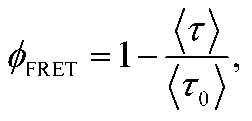 | (2) |
|
〈τ〉 = ∑Aiτi
| (3) |
The fluorescence decay curve of the donor in the presence of acceptors can be used as a tool to determine the distribution of donors and acceptors within the nanoparticle, since the resonance energy transfer is highly dependent on the donor–acceptor distance distribution.8 In this work we have made use of the treatment developed by Martinho's group,13,14 but slightly modified, which has been applied successfully to determine the dye distribution in different systems with spherical symmetry.11,15,16 The donor decay function after a delta-pulse excitation is given by:
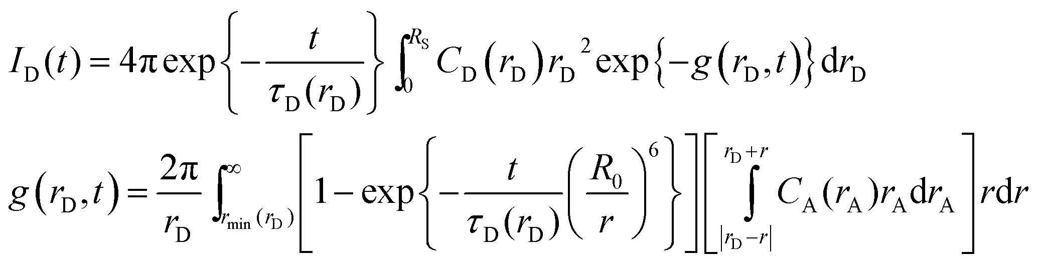 | (4) |
 | (5) |
In order to compare the theoretical predictions on the fluorescence decay curves ID(t), with the experimental ones Iexp(t), ID(t) is convoluted with the instrument response function L(t), to obtain:
 | (6) |
For simplicity of treatment, the dye distributions CD(rD) and CA(rA) introduced into eqn (4) will be based on combinations of step functions of the Heaviside type (H(r)). Detailed expressions for the donor decay functions for the different dye distributions used through the paper can be found in the ESI.†
Results and discussion
Experimental verification of shell growing
The core and the shells in the synthesized NPs are both polymeric, although their monomer compositions and structures (i.e., crosslinking degree) varies significantly in order to define layers with different properties such as polarity, hydrophobicity, solubility, free volume etc. The core is mostly comprised of MMA, HEMA and GMA, whereas the shells include as well EGDMA, a cross linking monomer (Table 1). In addition, the proportions of each monomer are different in the core and in the shell. For example, the MMA ratio in the shells is half that in the core. This implies that the shells are more prone to water swelling that the cores, but their increased polarity ensures a better environment for polar dyes such as Rh6G and NB.In order to start the growing of shells around the cores, it has to be guaranteed that the polymerization process of the latter has terminated. During the core synthesis, the dispersion of the monomer components by the presence of SDS molecules in the aqueous solution, and the full solubility of the hydrophilic monomer HEMA, leads to a fast polymerization which can be followed by monitoring the temperature inside the reactor (Fig. 1a), since the free radical polymerization is an exothermic reaction and raises the temperature of the solution. The maximum temperatures were achieved around 20 minutes after initiator addition, while after 45 minutes the reactor temperature was set at a constant value of 65 °C, indicating that the polymerization is almost finished. In fact, DLS measurements rendered identical particle diameters after 60 and 120 minutes of reaction (39.4 and 39.1 nm at 60 and 120 minutes, respectively, for sample RMS).
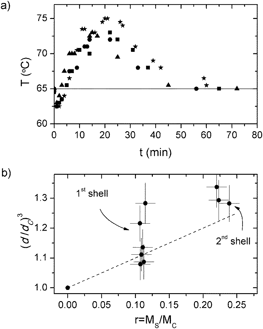 | ||
| Fig. 1 (a) Reactor temperature during core formation for four randomly chosen samples synthesized in this work (H, CS1, RMS and MS2). The solid line marks the set temperature of the reactor. (b) NP diameters against mass of the monomer feeds. The values have been rescaled by the diameter and monomer feed of the core particles. The error bars in (b) accounts for fluctuations inherent to the synthesis procedure and apparatus resolution. The dashed line represents the predicted NP diameter after each shell growth assuming the absence of polymer swelling enhancement, full monomer feed inclusion into the final particles, and similar copolymers densities in core and shells (i.e., (d/dC)3 = 1 + r). | ||
One of the aims of the present work is to assess the influence of the nanoparticle morphology on the optical properties of the system without interference by other parameters, which is a challenge due to the fact that in nano-sized systems several physicochemical parameters are entangled. Taking into account that the optical properties of nanostructured materials are strongly dependent on their final size, the NPs herein synthesized have a thin shell, ranging from 0.5 nm to 4 nm. Since the shell thickness is so small as compared to the core radius, any random variable affecting the particle growth introduces large uncertainties in the shell sizes. However, the growth of the different shells followed by performing DLS measurements after each monomer mixture addition (Table 1) allows us to establish some qualitative behavior. According to the data in Table 1, the NPs diameter grows with each new monomer addition. If all of the added monomer feed introduced in the flask to grow the shells (MS) were used to produced uniform and identical coatings over each NP, i.e., there were no new particles formed, the final particle diameter d should raise according to
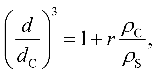 | (7) |
By measuring the particle diameter in each growth step, we could test the dependency of d on r, and the obtained results are shown in Fig. 1b. These results show that there is a positive correlation between these two parameters, being an indication that the size of the particles increases with the sequential addition of new monomer feeds, i.e., new shells are being form after each step. The dispersion observed in the values of d/dC for a constant value of r, 7% standard deviation for the first growth, falls within the expected experimental reproducibility of the synthesis we follow in this paper. However, the measured diameters are slightly larger than those predicted by eqn (7) assuming ρC/ρS ∼ 1 (Fig. 1b), indicating that the density of the shell would be lower than that of the core (ρC/ρS > 1). This could be ascribed to the water swelling in the shell resulting from the more hydrophilic nature of the monomers and compositions used for the shell, with respect to those of the core (MMA concentration in shell is half that in the core).
Even though, these results cannot fully confirm that all of the monomer feed added in the subsequent shell growths has been incorporated into the shells and, hence, they cannot rule out that a given fraction of the monomer has been turned into new particles or polymer solved in the interparticle medium.
Uncovering dye diffusion in core/shell NPs
The energy transfer process is highly dependent on the donor and acceptor distributions within the latexes, and may thus deeply affect the emission performance in these systems. Thus, it is important to correlate NP morphology (or dye distribution) with photophysical performance. Hence, our aim was to compare two different NPs with the same size and donor and acceptor concentrations (in terms of number of molecules within each NP), but with diametrically different dye distribution. Then, we synthesized two samples: latex NPs without shell and homogeneous donor and acceptor distributions (sample H, Table 1), and latex NPs with a core/shell morphology in which the donor dye Rh6G was placed at the core and the acceptor dye NB was placed at the shell (sample CS1, Table 1). Reference NPs without acceptor were prepared to extract information about the donor lifetime τD in the absence of acceptor and thus to calculate the FRET quantum yield ϕFRET with eqn (2) (samples RH and RCS, Table 1).As the mean distance between donors and acceptors in samples H and CS1 is highly distinct, one could expect a quite different behavior with respect to the FRET process, but the data in Table 2 and the fluorescence intensity decays of Rh6G in samples H and CS1 (Fig. 2a) suggested that there was not such a high difference, with samples H and CS1 presenting FRET efficiencies of 39% and 35%. In order to find the origin of this unexpected equality, we decided to fit the fluorescence intensity decays in Fig. 2a with theoretical expressions from which one can gather the donor and acceptor concentration distributions (see ESI†).
| Sample code | τi [Ai]a (ns) | 〈τ〉b (ns) | ϕFRETc (%) |
|---|---|---|---|
| a Fluorescence lifetimes (τi) and weights (Ai, ΣAi = 1) obtained from multiexponential fit of decay curve.b Amplitude average fluorescence lifetime of the donor subjected to FRET processes (eqn (3)).c FRET quantum yield. | |||
| H | 1.71 [0.45]; 3.64 [0.55] | 2.77 | 39 |
| RH | 3.11 [0.21]; 4.70 [0.79] | 4.37 | — |
| CS1 | 1.80 [0.45]; 3.87 [0.55] | 2.94 | 35 |
| CS2 | 1.55 [0.52]; 3.52 [0.48] | 2.50 | 45 |
| RCS | 4.52 [1] | 4.52 | — |
| MS1 | 1.48 [0.44]; 3.52 [0.56] | 3.01 | 35 |
| MS2 | 1.46 [0.43]; 3.50 [0.57] | 3.01 | 35 |
| RMS | 4.66 [1] | 4.66 | — |
 | ||
| Fig. 2 (a) Fluorescence intensity decays of Rh6G for sample H (black line) and CS1 (dark gray line). The light gray line is the instrument response L(t) after pulse excitation. The red and green lines are the best fits to CS1 and H decay data, respectively (Eqn (S10)–(S12) and eqn (S7)–(S9) have been used to samples CS1 and H, respectively). The blue line is the prediction of the core/shell model assuming CCA = 0 mM and CSA = 9.5 mM. Residuals of the fit to fluorescence decay of samples H and CS1 are plotted in (b) and (c), respectively. | ||
We began by evaluating the decay curve of sample H, as this kind of samples had been evaluated previously,11 and had been successfully fitted with the so called “core/surface” distribution (Model 1 in ESI; eqn. (S7)–(S9)†). In this scenario the NP consists of a homogeneous polymer core in which both donors and acceptors are homogeneously and uniformly solved, and an extremely thin shell (hairy layer) surrounding the core, in which both donors and acceptors are adsorbed. In the core/surface model, the fitting parameters are CSA and CCA (surface and volume densities of acceptors in surface (S) and core (C), respectively), and the constraint CCA/CSA = CCD/CSD applies (see ESI†). The reference sample RH shows two contributions to the lifetime of Rh6G in the NP (Table 2), the longest and main one being ascribed to the core (τD,C), and the shortest and residual one to the hairy layer (τD,S). Then, in eqn (S7) and (S8)† we used τD,C = 3.52 ns and τD,S = 1.55 ns. The best fit of eqn (S7)–(S9)† to the decay curve of Rh6G in sample H (χ2 = 0.5988, Fig 2a and b) rendered a total acceptor concentration CA = 2.4 mM, with 68% of all donor and acceptor molecules solved in the core, and the rest adsorbed in the surface.
The best fit overestimates the acceptor concentration in the NP with respect to the experimental value (CexpA ≈ 1.1 mM). At these donor concentrations (∼5.5 mM) the excitation energy migration due to homo FRET among donors increases the probability of energy transfer from Rh6G molecules to NB ones which otherwise would not have access to this excitation due to an excessive separation. In other words, the homo FRET among donors mediates in the hetero FRET between donors and distant acceptors. In fact, the presence of homo FRET in this particular system was previously demonstrated.11 As the used model (eqn (4)) does not account for this effect, and assumes that only the acceptor concentration governs the process, it “understands” the increase in the FRET efficiency due to the donors as an increase in the acceptor concentration, thus overestimating the latter. To modify the model considering the influence of homo FRET on the corresponding decay curves is neither a direct nor a simple task, but it would be necessary to enable gathering reliable information from highly loaded systems. Work is in progress in our labs towards this aim. Therefore, the information obtained from the fits is essentially qualitative, and must be treated as such.
Next, we evaluated the decay curve of sample CS1 by making use of a model considering a core/shell dye distribution (Model 2 in ESI; eqn (S10)–(S12)†), assuming that there were no donor in the shell (CSD = 0), and no acceptor in the core (CCA = 0), which were the targeted distributions. Hence, the only fitting parameter was CSA, the volume density of acceptors in the shell. In this case the reference sample RCS was a similar core/shell NP with donor molecules in the core but containing no dyes in the shell. Interestingly, the reference sample RCS shows only one contribution to the lifetime of Rh6G in the NP (Table 2), indicating that in the core/shell synthesis the surface dye population observed in the homogeneous NPs (sample RH) is not obtained. This means that somehow the shell growth is “cleaning” the hairy layer, or in other words, the newly included monomers drag the dyes in the surface to the inner part of the NP. For the sample CS1, the best fit of eqn. (S10)–(S12)† to the decay curve (χ2 = 0.6053, not shown) rendered a shell acceptor concentration CSA = 2.2 mM, much lower than the value expected from the dye loaded in the synthesis procedure (CSA = 9.5 mM). Indeed, the predicted fluorescence intensity decay for a core/shell NP assuming CSA = 9.5 mM and CCA = CSD = 0 in eqn (S10)–(S12),† presents a much higher de-excitation rate (Fig. 2a) and thus would imply a much higher FRET efficiency. This discrepancy could be owed to different reasons: (a) there is a NB leakage from the shell to the solution after/during synthesis or even that the dye is not properly included in the shell during the synthesis, and (b) the NPs do not present the assumed core/shell dye distribution.
The first reason could be ruled out, since we dialyzed the sample CS1 for 48 hours, and the absorption spectra of the aliquots from the cleaning water did not show evidences of either Rh6G or NB. To check the second reason, we run again the core/shell model fit (Model 2 in ESI; eqn (S10)–(S12)†) but this time letting CCD, CSD, CCA and CSA free. As the donor and acceptor molecules have a very similar nature (both chemical and electrostatic) they will have similar affinities for a given monomer mixture. Hence, we assume, for simplicity, that both dyes will present the same dye distribution within the core/shell NP, i.e., CCA/CSA = CCD/CSD. This constraint reduces the degrees of freedom to CCA and CSA. The best fit (χ2 = 0.5521, Fig. 2a and c) rendered a shell acceptor concentration CSA = 3.5 mM and a core acceptor concentration CCA = 1.7 mM, i.e., the 80% of all dye molecules ends up in the core. In addition, the fitted total concentrations are much closer to the experimental ones than those obtained with the homogeneous model (Model 1). This fit shows that, unexpectedly, both donors and acceptors are distributed along the whole NP, implying that there would be diffusion processes from the shell to the core, and vice versa, while or after the shell polymerization. Hence, the fact that both dye distributions in sample CS1 are “spread” through the NP, explains by itself the observed similitude between the fluorescence intensity decay curves, and in turn of ϕFRET, of samples H, fully homogenized, and CS1, partially homogenized.
The information on the core/shell morphology and on the diffusion process has to be considered only qualitatively. On the one hand, the complexity of the system makes practically impossible to model all the process involved in the energy transfer. On the other hand, the errors on the shell thickness affects the determination of dye concentrations in the model, as was discussed above. For this reason and to assure whether the observed dye diffusion was not a mere coincidence due to a particular problem during the synthesis of sample CS1, we synthesized another NP with core/shell morphology in which both donor and acceptor were placed at the core and the shell such that CCA ≈ CSA and CCD ≈ CSD (sample CS2, Table 1). Again, the best fit of eqn (S10)–(S12)† to the decay curve (χ2 = 0.4694, not shown) rendered a shell acceptor concentration CSA = 4.6 mM and a core acceptor concentration CCA = 1.8 mM. This means that the acceptor concentration in the shell is nearly twice and half as much as the dye concentration in the core, indicating again that dye diffusion took place.
Once proved that dye diffusion was taking place in our core/shell NPs, we wanted to know if the diffusion was finished or was in process. To assess that, we measured again the fluorescence intensity decay of Rh6G in sample CS1 several weeks after the first measurements, but no differences were found either on the ϕFRET value or the fluorescence intensity decays, indicating that the diffusion was finished or at least frozen.
Finally, trying to avoid or partially reduce the dye diffusion, we synthesized NPs with multiple shells; the core containing the donor, the outer shell containing the acceptor, and the inner shell(s), intended as dye barrier(s), containing no acceptor (samples MS1 and MS2, Table 1). Nonetheless, the outcome was analogous to that of sample CS1, i.e., there were important dye redistributions in the NPs due to free diffusion.
Then, it can be seen that the final dye distributions do not depend on the initial choice in the synthesis, but are governed by diffusion processes. The particular dye distributions obtained from the FRET decay curve fitting (acceptor concentrations in the shells 2 to 3 times higher than in the core) might be a consequence of the different solubilities of the dyes in the different regions. The shell contains more HEMA than the core (see Table 1), a monomer in which both Rh6G and NB have a higher solubility than in MMA monomer.18 In this sense, the dyes would be more “comfortable” in the shell than in the core, thus explaining the higher concentration in the former.
Theoretical evaluation of dye diffusion in core/shell NPs
To confirm the previous results and with the aim to have a clearer understanding of the diffusion processes within core/shell NPs (equilibrium and transient dye distributions, time scales, etcetera), we decided to analyze the behavior predicted by existing diffusion models. In this sense, Fick's second law19 predicts how diffusion causes the concentration of a given element to change in space and time for a given diffusion coefficient (dependent on the particular material properties). Since we are dealing with a chemical system in which every region—due to its different composition—presents a different affinity for the dyes, it is more adequate to work with chemical potentials. Fick's second law in spherical coordinates and in terms of chemical potentials reads (see ESI† for a detailed description on theoretical and numerical formalism used):
 | (8) |
|
μ(r,t) = μ0(r) + RTlnC(r,t).
| (9) |
In eqn (9), C(r,t) is the time-dependant volume number concentration (nm−3) of the diffusive element along the NP radius, μ0(r) is the reference chemical potential of a solution (μ0C in core and μ0S in shell), R = 8.31 J K−1 mol−1 is the gas constant and T = 300 K is the matrix temperature. Particle regions with large affinity for the dye (high solubility) will reduce the reference chemical potential and will enhance the dye concentration C(r,t).
All systems evolve to the equilibrium by compensating the differences in the chemical potentials along the system, i.e., at equilibrium μ(r) = constant ∀r. For our particular case, this equilibrium condition implies that Δμ0 = μ0C − μ0S = RTln(H), where H = CSeq/CCeq is the partition ratio and CSeq and CCeq are the equilibrium concentrations in the shell and core, respectively. Hence, by making use of the CSA and CCA values obtained from the fit to the fluorescence intensity decay of sample CS1 (Fig. 2a), it can be heuristically inferred that, in the particular case of this sample, Δμ0 ≈ RTln(2). For simplicity, the diffusion coefficient will be assumed constant along the NP with a value 10−16 cm2 s−1.
By numerically solving the above system of equations with the adequate initial and boundary conditions (see details in ESI†), the dye distribution profiles along the NP were obtained as a function of time both for acceptor and donor concentrations (Fig. 3). At the very beginning (t = 0 seconds in Fig. 3), the donor is fully contained in the core, and the acceptor in the shell. Only 50 milliseconds (Fig. 3) later, the acceptor population in the shell is significantly depleted and inhomogeneously distributed, being spread towards the core, where it presents a characteristic bell shaped diffusion profile. On the other hand, the donor population quickly fills the shell, showing a huge concentration discontinuity at the core/shell frontier. After 0.2 seconds (Fig. 3) from the start, the acceptor concentration in the shell is half of the initial and it shows a moderate homogeneity, while the donor concentration in the shell is already at the same level of the initial donor core concentration. Interestingly, in spite of the assumed restrictive diffusion coefficient, the system nearly reaches the equilibrium state just after 18 seconds, showing that CSA/CCA = CSD/CCD = 2, as was expected (Fig. 3). For completeness, the time evolution of the corresponding chemical potentials is shown in Fig. S1,† where it can be clearly observed that the system evolves to a state in which μ(r) is constant over the entire system (core and shell), as was already explained.
 | ||
| Fig. 3 Dye distribution profile along a NP analogous to CS1 as a function of time both for (a) the acceptor and (b) the donor. For better inspection, only the region around the core/shell transition is shown. The solid and dashed vertical lines indicate the position of the NP and core radii, respectively. | ||
Hence, the previous simulation confirms what was observed experimentally: the final dye distributions do not depend on the initial choice in the synthesis, but are governed by the reference chemical potentials of the different regions, or what is the same thing, by the affinity or solubility of the dyes in each monomer mixture. In this sense, the higher the solubility of the dye in a region is, the higher the final concentration in that region becomes. In our case, the distribution obtained from the FRET decay curve fitting and the previous numerical simulation, is consistent with the fact that the shell contains more HEMA than the core, a monomer in which both Rh6G and NB have a higher solubility than in MMA monomer.18
Since the real problem is looser with respect to the diffusion restriction, the equilibrium state will be reached experimentally in much less time. Taking into account that the shell growth needs a minimum of 60 minutes at 65 °C, the dye diffusion from core to shell, and vice versa, will be already over by the synthesis end.
Conclusion
In summary, we have shown that dye doped core/shell polymer NPs do not present always a well controlled dye concentration profile, as free dye diffusion may lead to important dye redistributions. In addition, we have made use of the FRET dynamics as a spectroscopic ruler to determine the particular dye profiles along the NPs, and have revealed the presence of dye diffusion in the core/shell NPs. This fact explains why the experimental measured FRET efficiencies are almost unaffected when changing in the synthetic route the dye distribution or the number of shells in the NP. In our particular case, in which core and shell are composed of methacrylic monomers, we have shown that the equilibrium concentration for both the donor and the acceptor in the shell is 2 to 3 times higher than that in the core, indicating that the dyes dissolve better in the monomeric mixture of the former, most probably for its higher HEMA content. The equilibrium state of this redistribution has been shown to be determined by the chemical potentials of the dyes in the different regions of the NPs, with the dyes accumulating preferentially in the region presenting the lower reference chemical potential (higher affinity or solubility). The information obtained from the theoretical model of dye diffusion in core/shell NPs suggests that the diffusion process from the shell to the core, and vice versa, takes place at the very beginning of the shell growth.In conclusion, if FRET-based multifunctional core/shell NPs are to be synthesized, the location where FRET is taking place (core, shell, or both) must be accurately controlled through a strict control of the dye diffusion. For example, by means of impermeable barriers between core and shell or covalently bonding the dyes to the monomers.
Acknowledgements
This work was funded by Spanish Ministerio de Economía y Competitividad (projects TRACE2009-0144, MAT2010-20646-C04-01 and MAT2010-20646-C04-04) and Gobierno Vasco (IT339-10). LGR thanks Gobierno Vasco for a predoctoral fellowship.Notes and references
- J. Shi, A. R. Votruba, O. C. Farokhzad and R. Langer, Nanotechnology in Drug Delivery and Tissue Engineering: from Discovery to Applications, Nano Lett., 2010, 10, 3223–3230 CrossRef CAS PubMed.
- A. S. Thakor, J. Jokerst, C. Zavaleta, T. F. Massoud and S. S. Gambhir, Gold Nanoparticles: A Revival in Precious Metal Administration to Patients, Nano Lett., 2011, 11, 4029–4036 CrossRef CAS PubMed.
- R. Taylor, S. Coulombe, T. Otanicar, P. Phelan, A. Gunawan, W. Lv, G. Rosengarten, R. Prasher and H. Tyagi, Small Particles, Big Impacts: A Review of the Diverse Applications of Nanofluids, J. Appl. Phys., 2013, 113, 011301 CrossRef PubMed.
- S. Wei, Q. Wang, J. Zhu, L. Sun, H. Lin and Z. Guo, Multifunctional Composite Core/Shell Nanoparticles, Nanoscale, 2011, 3, 4474–4502 RSC.
- R. Ghosh Chaudhuri and S. Paria, Core/Shell Nanoparticles: Classes, Properties, Synthesis Mechanism, Characterization, and Applications, Chem. Rev., 2012, 112, 2373–2433 CrossRef CAS PubMed.
- S. Luo, E. Zhang, Y. Su, T. Cheng and C. Shi, A Review of NIR Dyes in Cancer Targeting and Imaging, Biomaterials, 2011, 32, 7127–7138 CrossRef CAS PubMed.
- S. Santra, J. S. Xu, K. M. Wang and W. H. Tan, Luminescent Nanoparticle Probes for Bioimaging, J. Nanosci. Nanotechnol., 2004, 4, 590–599 CrossRef CAS PubMed.
- Principles of Fluorescence Spectroscopy, ed. J. R. Lakowicz, Kluwer Academic/Plenum Publishers, New York, 2nd edn, 1999 Search PubMed.
- E. Enciso, A. Costela, I. Garcia-Moreno, V. Martin and R. Sastre, Conventional Unidirectional Laser Action Enhanced by Dye Confined in Nanoparticle Scatters, Langmuir, 2010, 26, 6154–6157 CrossRef CAS PubMed.
- V. Martin, J. Bañuelos, E. Enciso, I. Lopez Arbeloa, A. Costela and I. Garcia-Moreno, Photophysical and Lasing Properties of Rhodamine 6G Confined in Polymeric Nanoparticles, J. Phys. Chem. C, 2011, 115, 3926–3933 CAS.
- L. Cerdán, E. Enciso, V. Martín, J. Bañuelos, I. López-Arbeloa, A. Costela and I. García-Moreno, FRET-Assisted Laser Emission in Colloidal Suspensions of Dye-Doped Latex Nanoparticles, Nat. Photonics, 2012, 6, 621–626 CrossRef.
- L. Cerdán, E. Enciso, A. Costela and I. García-Moreno, Random Lasing in Self-Assembled Dye-Doped Latex Nanoparticles: Packing Density Effects, Adv. Funct. Mater., 2013, 23, 3916–3924 CrossRef.
- A. Yekta, M. A. Winnik, J. P. S. Farinha and J. M. G. Martinho, Dipole-Dipole Electronic Energy Transfer. Fluorescence Decay Functions for Arbitrary Distributions of Donors and Acceptors. II. Systems with Spherical Symmetry, J. Phys. Chem. A, 1997, 101, 1787–1792 CrossRef CAS.
- J. P. S. Farinha and J. M. G. Martinho, Resonance Energy Transfer in Polymer Nanodomains, J. Phys. Chem. C, 2008, 112, 10591–10601 CAS.
- J. P. S. Farinha, M.-T. Charreyre, J. M. G. Martinho, M. A. Winnik and C. Pichot, Picosecond Fluorescence Studies of the Surface Morphology of Charged Polystyrene Latex Particles, Langmuir, 2001, 17, 2617–2623 CrossRef CAS.
- G. Marcelo, J. M. G. Martinho and J. P. S. Farinha, Polymer-Coated Nanoparticles by Adsorption of Hydrophobically Modified Poly(N,N-Dimethylacrylamide), J. Phys. Chem. B, 2013, 117, 3416–3427 CrossRef CAS PubMed.
- B. Bhattacharyya and B. K. Chakrabarti, The Mean Distance to the Nth Neighbor in a Uniform Distribution of Random Points: An Application of Probability Theory, Eur. J. Phys., 2008, 29, 639–645 CrossRef.
- A. Costela, I. García-Moreno and R. Sastre, Materials for Solid-State Dye Lasers, in Handbook of Advanced Electronic and Photonic Materials and Devices, ed. H. S. Nalwa, Academic Press, 2001, vol. 7, Liquid Crystals, Display and Laser Materials, pp. 161–208 Search PubMed.
- E. L. Cussler, Diffusion, Cambridge University Press, Cambridge, 1st edn, 1984 Search PubMed.
Footnote |
| † Electronic supplementary information (ESI) available. See DOI: 10.1039/c4ra02342k |
| This journal is © The Royal Society of Chemistry 2014 |