A strategy to achieve high electromagnetic interference shielding and ultra low percolation in multiwall carbon nanotube–polycarbonate composites through selective localization of carbon nanotubes

Abstract

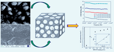
Here, we report a simple method that involves solution blending of polycarbonate (PC) in the presence of multiwall carbon nanotubes (MWCNTs) and commercial PC beads for the preparation of electrically conducting MWCNT–PC composites with high electromagnetic interference shielding effectiveness (EMI SE) and electrical conductivity at very low (∼0.021 wt%) percolation threshold (p_c). Thus, electrical conductivity of ∼4.57 × 10⁻³ S cm⁻¹ was achieved in the MWCNT–PC composites at an extremely low MWCNT loading (0.10 wt%) in the presence of 70 wt% PC beads in the composites. Finally, optimizing the ratio of PC beads and MWCNT loading in the composites, a very high EMI SE value (∼23.1 dB) was achieved at low loading (2 wt%) of MWCNT with 70 wt% PC beads. The effective concentration of MWCNT increases in the solution blended PC region with increasing the amount of PC beads. Thus, a strong interconnected conductive network structure of CNT–CNT is developed throughout the matrix and the presence of strong π–π interaction among the electron-rich phenyl rings of PC and MWCNT in the composites plays a crucial role in increasing the EMI shielding value and electrical conductivity of the MWCNT–PC composites.

---

1. Introduction

In last two decades, polymer has widely been used worldwide because of its high thermal and mechanical properties, high processability, easy handling and low cost.^1,2 However, in the conducting area, use of polymer is limited as most polymers are insulating in nature. In this regard, preparation of conducting polymer has been of great challenge in recent times. To overcome this problem, high electrically conductive nanofillers such as carbon black (CB), carbon nanofibres (CNFs), carbon nanotubes (CNTs) and graphene are incorporated in the insulating polymer matrix to make them electrically conductive. The electrically conductive polymer composites can be used in different fields of applications such as transistors,³ electronics,⁴ devices,⁵ automobiles, aerospace and EMI SE material.^6,7 The electrical and dielectric properties of polymer/conducting filler filled composites mainly depend on the type, shape, size and concentration of the nanofiller.

Recently, CNTs have been considered as the most promising nanofillers for the preparation of electrically conductive CNT–polymer composites due to their exceptionally high performance such as small size, high aspect ratio (length/diameter), large surface area and high electrical conductivity value.^8,9 However, the dispersion and distribution of CNT in the polymer matrix is difficult due to its high van der Waals forces. These forces lead to the agglomeration of CNT in polymer matrix. However, high surface area of the CNT is the key factor for developing good interaction between nanofiller and host polymer that reduces the CNT loading to achieve electrical conductivity in polymer composites. So, dispersion and distribution of the CNT is the main challenge for achieving high electrical conductivity in the composites at low CNT loading. The chemical modification or functionalization of the CNT may increase the interaction with polymer through better dispersion and interfacial adhesion of the CNT, but it creates surface defects which reduce the electrical conductivity of CNT in the final composites.

The dispersion of CNT in PC matrix is very difficult due to high melt viscosity of the PC. Consequently, high amount of CNT is required to achieve electrical conductivity in CNT–PC composites. Many researchers^10–14 have reported the EMI SE of various polymer composites using different nanofillers. For instance, Joo et al.¹⁰ reported the EMI SE of ∼27 dB at 40 wt% of MWCNT loading in solution blended purified MWCNT–poly(methyl methacrylate) (PMMA) composites. Gupta et al.¹¹ reported the EMI SE of ∼20 dB for the solution casted MWCNT–polystyrene (PS) composites at 7 wt% loading of MWCNT. Chen et al.¹² reported that the EMI SE of the solution blended single wall carbon nanotube (SWCNT)/polyurethane (PU) composites was ∼17 dB at 20 wt% loading of SWCNT. Gupta et al.¹³ achieved the EMI SE of ∼19 dB at 15 wt% loading of CNF in solution casted CNF–PS composites. Sundararaj et al.¹⁴ reported the EMI SE of ∼25.4 dB at 5 wt% of MWCNT loading in compression molded MWCNT–PS composites. Potschke et al.^15,16 have shown that the p_c of melt mixed MWCNT–PC composites prepared by diluting a MWCNT–PC mixture containing 15 wt% MWCNT was occurred in between 1 and 1.5 wt% of MWCNT loading. In addition, the chemical modification of CNT reduces the electrical conductivity of the CNT.

Khatua et al.^17–20 have already developed several PC–MWCNT conducting nanocomposites through melt-mixing with various polymer–MWCNT masterbatches, such as, PMMA,¹⁷ poly(ε-caprolactone) (PCL)¹⁸ those form miscible blends and acrylonitrile butadiene styrene (ABS),⁹ styrene acrylonitrile (SAN)¹⁹ and poly(butylene terephthalate) (PBT),²⁰ those form immiscible blends with the PC. They reported low percolation threshold of MWCNT in all these PC–MWCNT nanocomposites with high electrical conductivity. However, all these PC–MWCNT nanocomposites consist of a mixture of two different polymers, which provides the scope to develop PC–MWCNT conducting nanocomposites with very low percolation threshold of the MWCNT in PC matrix, without blending with other polymers.

In this study, we have developed a feasible method which involves solution blending of PC and MWCNT in the presence of commercial PC bead. Using this method, MWCNT was selectively localized in the solvent dried continuous PC phase. The PC bead in the continuous phase of the composites can be considered as excluded volume in which MWCNT can not penetrate. The effective concentration of the MWCNT thus increases with the addition of PC bead in the continuous region and hence increases the electrical conductivity of the composites. Through judicious control of MWCNT and PC bead content, very high EMI SE value (∼23.1 dB) was achieved at low loading of MWCNT (2 wt%) and a high electrical conductivity of ∼4.57 × 10⁻³ S cm⁻¹ was achieved at extremely low loading (0.10 wt%) of MWCNT in the presence of 70 wt% PC bead. Thus, through homogeneous dispersion and distribution of the MWCNT in the solvent dried continuous PC region, a continuous conductive interconnected network path of CNT–CNT has been developed throughout the matrix phase. This increases the π–π interaction among the electron rich phenyl rings of PC and MWCNT that helps to enhance the electrical conductivity of the composites.

2. Experimental

2.1. Material details

Amorphous PC (Lexan 143; density: 1.19 g cm⁻³; MFI: 10.5 g/10 min at 300 °C and 1.2 kg load) pellets (average diameter ∼2.75 mm and length ∼3.35 mm) were obtained from SABIC Innovative Plastics (formerly General Electric Plastics), Netherland. Industrial grade MWCNT (NC 7000 series; average diameter of 9.5 nm and length 1.5 μm; surface area 250–300 m² g⁻¹; 90% carbon purity) was purchased from Nanocyl S.A., Belgium. The MWCNT was used as received, without any further chemical modification.

2.2. Preparation of MWCNT–PC composites

At the beginning, PC beads (6 g) were dissolved in dichloromethane (DCM) solvent (15 ml) and MWCNT (0.005 g) was well dispersed in DCM solvent (15 ml) by ultra-sonication for 1 h in two different beakers. Then, the PC solution was added to the pre-dispersed suspension of DCM–MWCNT and ultra-sonicated for 1 h. The mixture of MWCNT–PC was stirred at 50 °C using magnetic stirrer for partial evaporation of DCM solvent. After 2 h of the stirring, when the MWCNT–PC mixture became pasty and highly viscous, 4 g of commercial PC beads was added into the viscous medium under constant stirring. Addition of the PC beads into the solution of MWCNT–PC at the initial stage (without partial evaporation of DCM) would result in swelling of the PC beads and thus, penetration of CNT inside the PC beads. Thus, the MWCNT–PC composites was obtained through solution blending of PC and MWCNT in the presence of commercial PC beads. The composites was first air dried and finally dried in an air oven at 100 °C for 16 h. From the weight (∼10 g) of the final product, calculated amount of the MWCNT and PC bead in the MWCNT–PC composites were 0.05 and 40 wt%, respectively. The (60/40 w/w) MWCNT–PC–PC composites with different MWCNT loadings (0.05, 0.08, 0.10 and 0.12 wt%) were prepared using the same method. The MWCNT–PC composites with higher amount of the PC beads (60 and 70 wt%) at different MWCNT loadings (0.05, 0.08, 0.10 and 0.12 wt%) were also prepared through the same route. Finally, MWCNT–PC composites were compression molded at 260 °C in a hot press under constant pressure (4 MPa) and the molded parts were air-cooled to room temperature for further characterizations. The schematic representation for the preparation of the composites is illustrated in Fig. 1.

Fig. 1 A schematic for the preparation of MWCNT–PC composites.

3. Characterization

3.1. Electrical conductivity

The direct current (DC) conductivity (σ_DC) measurement was done on the molded specimen bars of dimensions 30 × 10 × 3 mm³. The sample was fractured at two ends and the fractured surface was coated with silver (Ag) paste to ensure good contact of the sample surface with the electrodes. The electrical conductivity of the conducting composites was measured with a four-probe technique. The specimens were prepared under similar conditions to avoid the influence of the processing parameters on the electrical properties. Minimum of five tests were performed for each specimen and the data was averaged.

The frequency (f) dependent alternative current (AC) conductivity (σ_AC) and dielectric permittivity of the composites (disc type sample with thickness 0.3 cm and area 1.88 × 10⁻¹ cm²) were obtained using a computer controlled precision impedance analyzer (Agilent 4294A) by applying an alternating electric field (amplitude 1 volt) across the sample cell in the f region of ∼40 Hz to ∼10 MHz. A parallel plate configuration was used for all the electrical measurements. Molded disc type composites sample was coated with silver (Ag) paste to act as both side electrodes. After electroding, the samples were heated at 150 °C in air to impart better adhesion between the sample and contacts. A sample holder using Pt probe was used for all the electrical measurements.

The parameters like dielectric permittivity (ε′) and dielectric loss tangent (tan δ) were obtained as a function of f. The σ_ac was calculated from the dielectric data using the relation:

σ_ac ≈ ωε_oε′tan δ (1)

where, ω is equal to 2πƒ, and ε_o is vacuum permittivity. The dielectric permittivity (ε′) was determined with the following equation:

ε′ ≈ C_p/C_o (2)

where C_p is the observed capacitance of the sample (in parallel mode), and C_o is the capacitance of the cell. The value of C_o was calculated using the area (A) and thickness (d) of the sample, following the relation:

C_o ≈ (ε_o × A)/d (3)

3.2. EMI SE measurement

The EMI SE of MWCNT–PC composites was measured with E5071C ENA series network analyzer (Agilent Technologies) using an industrial standard method. Composites slabs of dimensions 25.5 × 13 × 5.6 mm³ were used for EMI SE measurement in the 8.2–12.4 GHz (the so called X band) frequency range.

3.3. Current (I)–voltage (V) measurement

I–V relationship in MWCNT–PC composites was measured with compression molded samples, using Keithley 2400 source meter (lab view 18.1 protocol). Both sides of the sample were coated with silver paste and the sample was placed on the probe station from where two contacts were taken out. Positive voltage was applied from the top contact of the material using the Keithley source meter.

3.4. Cyclic voltammetry (CV) analysis

Electrochemical study such as CV was performed by using three electrode systems where Pt wire and Ag/AgCl were used as counter and reference electrodes. The measurement of CV (Gamry Instrument, 750 mA and 2 V) was performed in 1 (M) KCl solution.

3.5. Raman spectroscopy measurement

Raman spectra of MWCNT and MWCNT–PC composites samples were studied with a Renishaw Raman microscope, equipped with a He–Ne laser excitation source emitting at a wavelength of 632.8 nm and a Peltier-cooled (−70 °C) charge-coupled device (CCD) camera. A Leica DMLM microscope was attached and fitted with three objectives (5×, 20×, 50×). The 20× objective was used in our study. The data acquisition time was 30 s. The slit provided a spectral resolution of 1 cm⁻¹.

3.6. Optical microscopy

High resolution optical microscope (HROM, Carl Zeiss Vision GmbH) was used to investigate the distribution of MWCNT in the PC matrix. Image from the surface of the compression molded sample was taken in monochromatic light at different resolutions.

3.7. High resolution transmission electron microscopy (HRTEM) analysis

The extent of dispersion of the MWCNT in the PC matrix was studied by HRTEM (JEM-2100, JEOL, Japan), operating at an accelerating voltage of 200 kV. The MWCNT–PC composites were ultra-microtomed under cryogenic condition with a thickness of around 60–90 nm.

3.8. Field emission scanning electron microscopy (FESEM) study

The surface morphology of the MWCNT–PC composites was studied using a Carl Zeiss-SUPRA™ 40 FESEM, with an accelerating voltage of 5 kV. The molded samples were kept in liquid nitrogen for 30–50 s in a stainless steel container and then broken inside the liquid nitrogen. The fractured surfaces of the samples were coated with a thin layer of gold (approx. 5 nm) to avoid electrical charging. The vacuum was in the order of 10⁻⁴ to 10⁻⁶ mm Hg during scanning and FESEM images were taken on the fractured surface of the sample.

3.9. Atomic force microscope (AFM) analysis

The morphology of the MWCNT–PC composites was verified by tapping mode AFM analysis of the cryo-fractured surface of the composites, using a Nanonics Multiview 1000TM (Israel) SPM system with a quartz optical fiber tip (diameter 20 nm and spring constant 40 N m⁻¹).

3.10. Dynamical mechanical analysis (DMA)

Thermo-mechanical properties of the MWCNT–PC composites were measured with a dynamic mechanical analyzer (DMA 2980 model, TA Instruments Inc., USA), using compression molded sample of dimension 30 × 6.40 × 0.45 mm³. The dynamic temperature spectra of the samples were obtained in tension film mode at a constant vibration f of 1 Hz, temperature range of 30–180 °C, at a heating rate of 5 °C min⁻¹ in N₂ atmosphere.

4. Results and discussion

4.1. Raman spectroscopy

The Raman spectra of the pure MWCNT and MWCNT–PC composites are shown in Fig. 2. This characterization was done with visible (632.8 nm) laser light. From the figure, it is clearly observed that the characteristic peaks for MWCNT were appeared at ∼1331 cm⁻¹ (1D band) and ∼1604 cm⁻¹ (1G band). The peak for D band was raised for the breathing modes of sp² atoms in the rings and the G peak was developed due to the bond stretching of all pairs of sp² atoms in both the rings and chains, which are well known as the disorder induced and in plane E_2g zone center modes, respectively.²¹ However, in the case of MWCNT–PC composites, it is clearly seen that the intensity of the D (ID) and G (IG) bands was higher than that of pure MWCNT. The 1D/1G ratio for MWCNT–PC composites is higher than that of MWCNT. This high ratio of 1D/1G in MWCNT–PC composites indicates the formation of possible covalent bonds between PC and MWCNT, which partially breaks the sp² carbon network and makes a strong interaction among them.

Fig. 2 Raman spectrum analysis of MWCNT and MWCNT–PC composites.

4.2. Morphology

The morphology of the MWCNT–PC composites was studied through HROM, FESEM and HRTEM analysis, as shown in Fig. 3. Fig. 3a represents the optical micrograph image of the MWCNT–PC composites containing 0.10 wt% of MWCNT in the presence of 70 wt% PC beads. The optical image clearly shows the two phase regions; the transparent regions in the image represent the PC bead without any MWCNT, and the continuous opaque section stands for the solution blended MWCNT–PC phase. The presence of biphasic region confirms the existence of PC beads in the solvent dried MWCNT–PC continuous region of the MWCNT–PC composites. However, a slight reduction in bead size of the PC was evident in the optical image of the composites. This could be due to partial swelling and thus, surface etching of the beads to some extent by the solvent during composites preparation. If this is true, one would expect more surface etching and hence significant reduction in bead size when the composites were prepared with relatively low loading of the PC bead, using same amount of the solvent. To check this, we compared the optical images of MWCNT–PC composites, prepared with the same method, containing 0.10 wt% of MWCNT in the presence of 60 wt% (Fig. 1Sa†) and 40 wt% PC bead (Fig. 1Sb†), which are shown in ESI.† As evident, the size of the beads (white regions) in optical images of the composites with 60 wt% and 40 wt% PC bead is smaller as compared to that in case of the composites with 70 wt% PC bead.

Fig. 3 (a) Optical micrograph, (b and c) FESEM micrographs at two different magnifications, and (d) HRTEM micrograph of MWCNT–PC composites with 70 wt% PC bead and 0.10 wt% MWCNT loading.

Fig. 3b and c represent the FESEM micrographs of the MWCNT–PC composites containing 0.10 wt% MWCNT in the presence of 70 wt% PC bead. The FESEM image in Fig. 3b perceptibly demonstrates two phase regions. The MWCNT is assumed to be presented in the solvent dried MWCNT–PC continuous region and the PC beads dispersed in the continuous region. We assumed that the MWCNT failed to penetrate inside the PC beads during solution blending of PC and MWCNT in the presence of PC beads. Thus, MWCNT was selectively dispersed in the solvent dried PC region, outside the PC beads. A higher magnification image (Fig. 3c) of the selected area in Fig. 3b clearly revealed the homogeneous distribution and individualization of the MWCNT in the continuous PC matrix. From HRTEM image (Fig. 3d), random distribution of high aspect ratio tube like structures (d ≈ 25–30 nm) clearly indicated the individualization of the MWCNTs with retention of their aspect ratio (without much breaking or damage of nanotubes) during the composites preparation and melt-compression. MWCNTs were selectively confined in the solution blended continuous PC region, and thus, formed a continuous conductive interconnected network pathway of CNT–CNT throughout the PC matrix.

Fig. 4 shows the 2D and 3D AFM images of the cryo-fractured surface of MWCNT–PC composites with 0.10 wt% MWCNT loading and 70 wt% PC bead. From the images (Fig. 4a and b), it is clearly seen that the MWCNT was well dispersed and distributed in the selective region of the composites. We assume that, MWCNT was located selectively in the solution blended PC phase in the composites, leaving the PC beads free from any CNT.

Fig. 4 (a) 2D and (b) 3D AFM images of MWCNT–PC composites with 0.10 wt% MWCNT loading and 70 wt% PC bead.

4.3. EMI SE measurement

The EMI SE of the conductive polymer composites is strongly dependent on its σ_DC. The EMI SE of a material is mathematically represented by the following equation:

EMI SE (dB) = 10 log(P₀/P_t) (4)

where, P₀ is the incident and P_t is the transmitted or remaining electromagnetic power.

The incident power (P₀) is divided into reflected power (P_r), the absorbed power, and the remaining power (P_t) at the output of the shielding.²² The variation of the EMI SE with f in the region of 8.2–12.4 GHz (X band region) for the MWCNT–PC composites with different MWCNT and bead loadings is shown in Fig. 5. As observed, the EMI SE of the composites increased with increasing the MWCNT loading at a constant f region. It is noteworthy; the MWCNT–PC composites with 2 wt% of MWCNT loading and 70 wt% PC bead exhibited the EMI SE value of ∼23.1 dB at X-band region. This unprecedented shifting of the EMI SE to a higher value (∼23.1 dB) at very low MWCNT loading in MWCNT–PC composites is attributed mainly to the formation of conducting interconnected continuous network of CNT–CNT in insulating PC matrix that interacts with the incident radiation and leads to the higher EMI SE. The nano-sized MWCNT provides a larger interfacial area and high aspect ratio (L/D) of the CNT helps to generate extensively continuous interconnected network structures that facilitates electron transport in the composites at very low nanofillers loading (2 wt% MWCNT). The minimum value of the EMI SE of the composites for commercial applications is around 20 dB (i.e., equal to or less than 1% transmission of the electromagnetic wave). Thus, this investigation indicates that MWCNT–PC composites with 2 wt% MWCNT loadings and 70 wt% PC bead can meet the requirement of commercial applications. When electromagnetic radiation is incident on a slab of material, the absorptivity (A), reflectivity (R), and transmissivity (T) must sum to the value “one”, that is,

T + R + A = 1 (5)

Fig. 5 EMI Shielding vs. frequency of the MWCNT–PC composites containing different MWCNT loadings at 70 wt% PC beads content.

The absorptivity (A), reflectivity (R), and transmissivity (T) coefficients were obtained by using S parameters, as given below:

T = [E_T/E_I]² = |S₁₂|² = |S₂₁|² (6)

R = [E_R/E_I]² = |S₁₁|² = |S₂₂|² (7)

The total EMI SE (SE_total) is the sum of the reflection from the material surface (SE_R), the absorption of electromagnetic energy (SE_A), and the multiple internal reflections (SE_M) of electromagnetic radiation, as written below:

SE_total = SE_A + SE_R + SE_M (8)

The reflection is related to the impedance mismatch between air and absorber, the absorption can be regarded as the energy dissipation of the electromagnetic microwave in the absorber, and the multiple reflections are considered as the scattering effect of the in-homogeneity within the materials. When SE_total ≥ 15 dB, it is usually assumed that SE_M is negligible, and thus,

SE_total ≈ SE_A + SE_R (9)

The effective absorbance (A_eff) can be described as,

A_eff = (1 − R − T)/(1 − R) (10)

With respect to the power of the effective incident electromagnetic wave inside the shielding material, the reflectance and effective absorbance can be conveniently expressed as,²³

SE_R = −10 log(1 − R) (11)

SE_A = −10 log(1 − A_eff) = −10 log[T/(1 − R)] (12)

Using the equations given below,

SE_R = −10 log R (13)

SE_total = −10 log T (14)

A = 1 − T − R (15)

we can therefore get the value of absorptivity (A), reflectivity (R), and transmissivity (T). In this work, for the MWCNT–PC composites with 2 wt% MWCNT loading and 70 wt% PC bead, the reflectivity (R), absorptivity (A), and transmissivity (T) are 0.79, 0.204, and 0.006, respectively, at 8.2 GHz. Thus, the contribution of reflection to the total EMI SE is much larger than that from absorption. That means, the primary EMI SE mechanism of such type of composites is reflection rather than the absorption in the X-band region. This investigation suggests that the MWCNT–PC composites could be considered as a potential composites material for the shielding applications such as in construction of light weight shielding room, etc.

4.4. σ_DC measurement

The variation of σ_DC of the MWCNT–PC composites with different amounts (0–70 wt%) of PC beads at a constant MWCNT loading (0.05 and 0.10 wt%) is shown in Fig. 6a. As can be seen, the value of σ_DC of the MWCNT–PC composites (with 0.05 and 0.10 wt% MWCNT loadings) increases with increasing the PC bead loading. The value of σ_DC of the MWCNT–PC composite was ∼8.27 × 10⁻⁴ S cm⁻¹ when the composites was prepared without any PC bead at 0.10 wt% MWCNT loading. However, the value of σ_DC of the composites was increased with the addition of PC bead during solution blending of PC and MWCNT and σ_DC of ∼2.15 × 10⁻³ S cm⁻¹ was achieved when the composites was prepared with 60 wt% of PC bead at a similar MWCNT loading. Furthermore, the value of σ_DC of the composites was gradually increased with increasing the PC bead loading (up to ∼70 wt%) during solution blending. Similar kind of electrical conductivity in the MWCNT–PC composites was also observed for all the MWCNT–PC composites containing various amounts (0.05, 0.08, 0.10 and 0.12 wt%) of MWCNT.

Fig. 6 (a) DC conductivity of MWCNT–PC composites at different weight percent of PC bead in the PC matrix with various MWCNT loadings. (b) DC conductivity of MWCNT–PC composites with MWCNT loading. The log–log plot of σ_DC versus (p − p_c) for the composites was shown in inset of Fig. 5a. The straight line in the inset is a least–squares fit to the data using eqn (16), giving the best fit values p_c = ∼0.021 and t = ∼3.21.

The presence of PC beads in the PC matrix phase increased the effective concentration of the MWCNT in the solvent blended continuous PC region. The PC beads in the continuous phase of MWCNT–PC composites can be regarded as “excluded volume”, in which the MWCNT can not penetrate, resulting a high effective concentration of the MWCNT in the solution blended MWCNT–PC phase. Thus, the high effective concentration of the MWCNT in the solution blended and solvent dried PC phase plays a key role for achieving high electrical conductivity of the composites at an extremely low loading (0.05 wt%) of MWCNT. Thus, high σ_DC of the MWCNT–PC composites was achieved with increasing the content of PC beads in the composites.

The σ_DC of the MWCNT–PC composites without PC bead at different loading (0.05, 0.08, 0.10 and 0.12 wt%) of MWCNT is shown in Fig. 6b. As observed, the value of σ_DC of the MWCNT–PC composites gradually increased with increasing the MWCNT loading in the PC matrix. It was noteworthy, the value (∼4.35 × 10⁻⁵ S cm⁻¹) of σ_DC for MWCNT–PC composites was very high even at extremely low loading (∼0.05 wt%) of MWCNT. The value of σ_DC of the MWCNT–PC composites was ∼3.09 × 10⁻⁴ S cm⁻¹ at 0.08 wt% of MWCNT loading and that of ∼8.27 × 10⁻⁴ S cm⁻¹ at 0.10 wt% of MWCNT loading.

This very high value of σ_DC of the MWCNT–PC composites can be described due to the development of the continuous conductive interconnected network structure of CNT–CNT throughout PC phase even at extremely low MWCNT loading. At the beginning, σ_DC value of the MWCNT–PC composites containing 0.001 wt% MWCNT loading was ∼1.1 × 10⁻¹⁴ S cm⁻¹, which is almost similar to the conductivity value of insulating pure PC. However, the value of σ_DC of the MWCNT–PC composites was enormously changed when the composites were prepared with 0.05 wt% loading of MWCNT and a very high σ_DC of ∼4.35 × 10⁻⁵ S cm⁻¹ was achieved. Thus, σ_DC value was rapidly jumped by several orders (∼10⁹ order) of magnitude from 10⁻¹⁴ to 10⁻⁵. This rapid change in the value of σ_DC clearly indicates the formation of continuous interconnected conductive network chains of CNT–CNT in the composites, known as percolation network.

Many researchers^7,24 predicted the variation of σ_DC value with the different weight percent (p) of nanofiller in conducting polymer composites on the basis of percolation theory. According to the percolation theory, the transition occurred from insulating materials to conductor at a particular concentration of the conducting nanofillers, known as critical concentration. At this concentration, amount of nanofiller is sufficient for the formation of a continuous interconnected conductive network through the insulating host polymer. The lowest concentration of the conducting nanofiller from which composites shows a sudden rise in electrical conductivity is known as the p_c. Thus, the value of σ_DC of the polymer composites can be expressed with the term of p and p_c near the p_c with the help of following scaling law equation:

σ_DC(p) ∝ (p − p_c)^t for p > p_c (16)

where, ‘t’ stands for critical exponents. The ‘t’ values change with the value of p_c and also the dimensionality of the polymer composites.²⁵ A well fitted linear plot of log σ_DC vs. log(p − p_c) has been plotted to calculate the values of ‘t’ and ‘p_c’ for the MWCNT–PC composites by using the eqn (16), as shown in the inset of Fig. 6b. The calculated values of ‘t’ and p_c for the MWCNT–PC composites were ∼3.21 and ∼0.021 wt% loading of MWCNT, respectively. This very low p_c value (∼0.021 wt% MWCNT) indicates a homogeneous dispersion and distribution of the stick like MWCNT in the MWCNT–PC composites and presence of a strong π–π interaction between the phenyl ring of PC and electron rich MWCNT, as schematically shown in Fig. 7.

Fig. 7 A schematic for the possible π–π interactions between MWCNT and PC in the MWCNT–PC composites.

The very low p_c value of the composites can be explained by several factors,^26,27 such as, (i) high aspect ratio of MWCNT bundles which helps to reduce the p_c value, (ii) higher structure factor of the MWCNT due to its different lengths and an irregular packing which enhances the entanglements of MWCNTs with neighboring nanotubes. These higher structure factors of the MWCNT may help to reduce the p_c value, (iii) very high surface area of the MWCNT leads to a greater probability of conductive tunneling between the nanotube bundles and decrease the p_c value, (iv) the MWCNT bundles which extending out beyond a surface of bundles is very flexible. Thus, flexible MWCNT can make easy physical entanglements with adjacent nanotubes through small attractive forces which reduce the p_c value remarkably.

Balberg et al.²⁸ assumed the p_c in terms of average excluded volume (L/R) by the following equation:

p_c(L/R) ≈ 3 (17)

where, L represents the length of the randomly oriented stick like nanofillers and R signifies the radius of the stick nanofillers. This may give an idea for the average aspect ratio of the CNT bundles. These bundles may be made by the aggregation of the individual CNT and its size thus indicates the dispersion of nanofiller. Considering the average length and diameter of MWCNT as 1.3 μm and 9.5 nm, respectively (i.e. data given by MWCNT producer), the L/R value becomes ∼150 and using the eqn (17), the calculated value of p_c becomes near about 0.02. However, in our study, obtained p_c value is ∼0.021, and thus, the calculated value of L/R is ∼143. Thus, this study reveals that MWCNT contains an unknown number of nanotubes which may result in the bundles having longer than 1.3 μm and diameter greater than 9.5 nm. This result confirms that electrical conductivity in the MWCNT–PC composites is mainly arising due to CNT bundles.

According to percolation theory,²⁹ an infinite cluster of interconnected conductive network path of nanofillers has been formed at the critical concentration throughout the polymer matrix. Two particles are supposed to be connected when they are in physical contact. Electrical conductivity of the conducting polymer composites is higher than that of the insulating polymer before formation of a continuous network path of nanofillers in the composites. This kind of electrical conductivity in the composites is developed due to an inter-particle conduction mechanism. Grossiord et al.³⁰ have reported that the tunneling mechanism is one of the reasons for the development of electrical conductivity in polymer composites. Ryvkina et al.³¹ have discussed the electron tunneling mechanism on the basis of theoretical model of the polymer–CB composites, with the help of the following equation:

σ_DC ∝ exp(−Ad) (18)

where, A represents the tunnel parameter and d stands for tunnel distance. The existence of tunneling conduction mechanism for different composites has been well explained by several groups.^32,33 According to tunneling conduction mechanism, the charge carriers move through the polymer composites across insulating gaps between the nanofillers. Thus, electrical conductivity of the composites varied depending on the existence of tunneling conduction which contributes to the current through the composites.³⁴ The energy barrier of the composites strongly depends on the nature of the polymer matrix, as well as, the fabrication process. The current in a tunnel junction decreases with the barrier width. If the nanofillers are randomly distributed throughout the matrix, then the mean average distance (d) between the nanofillers would be considered as barrier width (d), which is directly proportional to the nanofiller concentration in weight, p^−1/3 considering the first approximation value by the following equation:³⁵

d ∝ p^−1/3 (19)

Thus, the summation of eqn (18) and (19), the tunneling assisted conductivity (log σ_DC) can be expressed in terms of p^−1/3 by the following equation:

log(σ_DC) ∝ p^−1/3 (20)

Using the eqn (20), log σ_DC vs. p^−1/3 has been plotted for MWCNT–PC composites and a linear variation of plot was obtained, as shown in Fig. 8a. This linear plot confirms the existence of tunneling mechanism in the composites which is responsible for the development of the electrical conductivity. According to Kilbride et al.,³⁶ individual conductive nanofiller was coated by insulating polymer which reduced the electrical contact among the nanofillers in the polymer composites and thus, increased the contact resistance between the nanofillers. So, tunneling of the electrons among the adjacent MWCNT occurs through very thin layer of insulating polymer and can not move from one electrode to another due to high energy barrier. However, this high energy barrier decreases by applying the voltage between the two electrodes. This acts as the driving force for the movement of electrons to overcome the energy barrier by tunneling conduction. Hence, the contact resistance between the nanofillers greatly reduces and enhances the electrical conductivity of the polymer composites. The variation of AC electrical conductivity (σ_AC) (Fig. 2S†) and dielectric permittivity (ε′) (Fig. 3S†) with frequency (f) for the MWCNT–PC composites are available in ESI† section.

Fig. 8 (a) Plot of σ_DC versus p^−1/3 for MWCNT–PC composites and (b) comparison of our result with reported electrical conductivity value of MWCNT–PC composites, prepared by various methods.

The literature reported values for σ_DC of the MWCNT–PC composites prepared by different methods such as solution blending and melt-mixing of PC with different MWCNT loading are shown in Fig. 8b and compared with our σ_DC value. Kim et al.³⁷ prepared MWCNT–PC/poly(3-hexylthiophene)-g-polycaprolactone (P3HT-g-PCL) composite films through solution blending with different MWCNT loadings. The electrical conductivity of the composites was ∼1.4 × 10⁻³ S cm⁻¹ at 0.5 wt% MWCNT loading. Lee et al.³⁸ prepared H₂O₂ treated-MWCNT–PC composites through solution blending. The σ_DC of ∼2.06 × 10⁻⁴ S cm⁻¹ was achieved in the composites at 0.5 wt% H₂O₂ treated MWCNT loading. Wu et al.³⁹ have observed σ_DC of ∼2 × 10⁻⁸ S cm⁻¹ at 2 wt% loading of carboxylic acid functionalized MWCNT in MWCNT–PC composites, prepared by diluting solution blended carboxylic acid functionalized MWCNT (10 wt%)/PC mixture followed by melt blending. Joo et al.⁴⁰ prepared MWCNT–PC composites through melt blending and an electrical conductivity of ∼10⁻² S cm⁻¹ was achieved at 2.5 wt% MWCNT loading. King et al.⁴¹ prepared MWCNT–PC composites through melt blending with different MWCNT loading. The σ_DC of the composites was ∼5.5 × 10⁻² S cm⁻¹ at 6 wt% MWCNT loading. It is noteworthy, the value of σ_DC of the MWCNT–PC composites prepared by our proposed method is very high (∼4.57 × 10⁻³ S cm⁻¹) than the σ_DC values of the conventional melt and solution blended MWCNT–PC composites reported till date and this high σ_DC value was obtained at exceptionally low MWCNT loading (0.10 wt%) with 70 wt% PC bead. The PC beads in the matrix phase act as excluded volume where MWCNT fails to penetrate and thereby increase the effective concentration of MWCNT in the solution blended (solvent dried) PC region.

4.4.1. Pressure and temperature dependent σ_DC. The pressure dependent σ_DC of the MWCNT–PC composites with 0.1 wt% MWCNT and 70 wt% PC bead is shown in Fig. 9a. As observed, the σ_DC of the composites gradually increases with increasing the molding pressure. In the highly conducting MWCNT–PC composites, the conducting nanofillers are separated by a thin film of insulating polymer matrix. The mechanism of charge transport has a strong effect on the electrical conductivity with the application of pressure. Generally, electrical conductivity of the composites occurred through direct contact between nanofillers and hopping or tunneling through the matrix polymer separating the adjacent nanofillers. At certain concentration of the nanofillers, the inter-particle gap between nanofillers become small enough to come close to or contact each other and formed a conducting network path throughout the host polymer. Due to application of external pressure on the composites, this local conductive path can easily penetrate into the insulating polymer matrix and develops effective conducting path in the composites. The variation of the electrical conductivity of the composites with molding pressure can be explained by different mechanisms.⁴²

Fig. 9 The variation of DC conductivity of MWCNT–PC composites with (a) pressure, (b) high temperature and (c) low temperature. The composites in (b) and (c) were prepared with a molding pressure of 4 MPa.

(a) The gap between two adjacent nanofillers become smaller by applying the uniaxial pressure which decreases the electrical resistance of one effective conductive path and leads to an increase in the tunneling current and electrical conductivity of the composites.

(b) The inter-particle distance between adjacent nanofillers decreases when compressive pressure increases, which helps to increase the formation of new effective conductive network paths throughout the matrix.

(c) The nanofillers are incompressible compared to the polymer. Therefore, application of pressure can induce translation and rotation of nanofillers. The nanofillers can be redistributed and reoriented within the insulating matrix due to transverse slippage. This effect has two opposite phenomena:

(i) The effective interconnected conductive paths in the composites can be destroyed or the number of conductive paths can be reduced.

(ii) The other phenomena are that more effective conductive network paths can be formed due to the redistribution or reorientation of the nanofillers in the composites.

The variation of σ_DC of MWCNT–PC composites with temperature are shown in Fig. 9b and c. From Fig. 9b, it is clearly seen that the σ_DC of MWCNT–PC composites gradually increases with increasing temperature which indicates the semiconducting behavior of the composites. This change of electrical conductivity of the composites with temperature occurred due to the increase in electronic movement of the nanofillers which plays a key role to increase the electrical conductivity of the composites. The energy barrier among the nanofillers is gradually reduced with increasing the temperature and acts as a driving force for the movement of electrons across the barrier by tunneling conduction. Thus, electrons in the polymer composites tunnel from one electrode to the adjacent electrodes which decrease the tunneling resistance and increase the electrical conductivity of the composites. Fig. 9c shows the effect of low temperature on the σ_DC of the composites and the value of the σ_DC decreases with decreasing the temperature. The electronic movement of the nanofillers decreases with decreasing the temperature. The energy barrier gradually increases with decreasing the temperature among the nanofillers which resist the movement of the electrons through the barrier by tunneling conduction. When the inter-particle separation is very large, no current flows through the inter-particle separation. Thus, the electrical conductivity of composites gradually decreases.

Fig. 10 represents the schematic for the formation of conductive paths in the composites under the application of external pressure. When pressure is applied on the composites, the conductive path is established which helps to enhance the electrical conductivity in the composites. In conducting polymer composites, the total electrical conductivity is the summation of conductivity of individual conducting nanofiller and the matrix polymer. The electrical conductivity of conducting nanofillers is very high compared to that of the matrix polymer. So, the resistance across the conducting nanofillers can be neglected. When the inter-particle separation of the nanofillers is very small, the tunneling current may flow through the separation and increases the electrical conductivity of the composites.

Fig. 10 A schematic for the formation of conductive paths in the composites under the application of external pressure.

4.5. I–V relationship

The I–V relationship for MWCNT–PC composites containing 0.1 wt% MWCNT and 70 wt% PC bead was measured at room temperature (303 K) within the potential window of −5 V to +5 V and shown in Fig. 11. A nonlinear increase in current was observed with the applied voltage, indicating a non-ohmic behavior of the MWCNT–PC composites. This nonlinear nature of the MWCNT–PC composites indicates the semiconducting behavior.⁴³ Thus, this material can be used in different electronic devices.

Fig. 11 I–V characteristics of MWCNT–PC composites.

4.6. CV analysis

Cyclic voltammograms of MWCNT–PC composites with 0.1 wt% of MWCNT loading and 70 wt% PC bead is shown in Fig. 12. Electrochemical study (CV) was carried out by using three electrode systems where MWCNT–PC composites, Pt wire and Ag/AgCl (KCl saturated; +197 mV) served as working, counter and reference electrodes, respectively. The composites was analyzed with in the potential windows of 0–1.0 V. CV measurements were performed in 1 (M) KCl solution at a scan rate of 30 mV s⁻¹. The specific capacitance (C_sp) was calculated by the following equation.^44,45

C_sp = (I₊ − I₋)/v × m (21)

where, I₊ and I₋ are the maximum currents in positive and negative voltage scan, respectively; v is the scan rate and m is the mass of the MWCNT–PC composites. The electrodes were used for electrochemical characterization without any polymer binder.

Fig. 12 Cyclic voltammogram of MWCNT–PC composites at a scan rate of 30 mV s⁻¹.

The specific capacitance of the MWCNT–PC composites was ≈117 F g⁻¹. As shown in FESEM and TEM images (Fig. 3), uniform distribution and homogeneous dispersion of MWCNT in selective region of the polymer matrix enhanced the specific capacitance due to the synergetic effect of MWCNT. The storage modulus of the MWCNT–PC composites is available in ESI section (Fig. 4S†).

5. Conclusion

In conclusion, we have reported a simple method that involves solution blending of PC and MWCNT in the presence of commercial PC beads for the preparation of high EMI SE and electrically conductive MWCNT–PC composites. A very high EMI SE value (∼23.1 dB), which is above the commercially applicable EMI SE value (20 dB), was achieved in the MWCNT–PC composites at very low loading (2 wt%) of MWCNT using 70 wt% PC bead during preparation of the composites. The value of σ_DC of the composites increases with increasing the PC bead content in the composites. The insulating PC bead acts as excluded volume in which MWCNT fails to penetrate, and thus increases the effective concentration of MWCNT in the continuous PC region. Thus, net σ_DC of the composites increases with the addition of PC bead at constant MWCNT loading. The obtained p_c value for the composites prepared by this method is very low (∼0.021 wt%) and the linear variation of log σ_DC versus p^−1/3 indicates that involvement of tunneling conduction between MWCNT is the reason behind the high electrical conductivity. Morphological analysis reveals the homogeneous and random dispersion of MWCNT in the solution blended continuous PC region and forms a continuous conductive interconnected network structure of CNT–CNT. The I–V study of the composites indicated the semiconducting nature of the composites and shows specific capacitance value of ∼117 F g⁻¹ at 30 mV S⁻¹ scan rate. The storage modulus of the composites also increases in the presence of small amount MWCNT as well as PC bead. The MWCNT–PC composites can be used in different field of applications such as light weight shielding room, mobile cell, spacecraft and aerospace etc.

Acknowledgements

We thank the Council of Scientific and Industrial Research (CSIR), New Delhi, India for their financial support.

References

1. C. Y. Li, L. Li, W. Cai, S. L. Kodjie and K. K. Tenneti, Adv. Mater., 2005, 17, 1198.
2. F. Flandin, T. Prasse, R. Schueler, K. Schulte, W. Bauhofer and J. Y. Cavaille, Phys. Rev. B: Condens. Matter Mater. Phys., 1999, 59, 14349.
3. J. Geng and T. Zeng, J. Am. Chem. Soc., 2006, 128, 16827.
4. P. Gajendran and R. Saraswathi, J. Phys. Chem. C, 2007, 111, 11320.
5. L. Ci, J. Suhr, V. Pushparaj, X. Zhang and P. M. Ajayan, Nano Lett., 2008, 8, 2762.
6. Y. Tang, B. L. Allen, D. R. Kauffman and A. Star, J. Am. Chem. Soc., 2009, 131, 13200.
7. H. Y. Chiu, P. Hung, H. W. C. Postma and M. Bockrath, Nano Lett., 2008, 8, 4342.
8. M. Moniruzzaman and K. I. Winey, Macromolecules, 2006, 39, 5194.
9. S. Maiti, N. K. Shrivastava and B. B. Khatua, Polym. Compos., 2013, 34, 570.
10. J. Joo, H. M. Kim, K. Kim, C. Y. Lee, S. J. Cho, H. S. Yoon, D. A. Pejakovic, J. W. Yoo and A. J. Epstein, Appl. Phys. Lett., 2004, 84, 589.
11. Y. Yang, K. L. Dudley, R. W. Lawrence and M. C. Gupta, Nano Lett., 2005, 5, 2131.
12. Z. Liu, G. Bai, Y. Huang, Y. Ma, F. Du, F. Li, T. Guo and Y. Chen, Carbon, 2007, 45, 821.
13. M. C. Gupta, Y. Yang, K. L. Dudley and R. W. Lawrence, Adv. Mater., 2005, 17, 1999.
14. M. Arjmand, T. Apperley, M. Okoniewski and U. Sundararaj, Carbon, 2012, 50, 5126.
15. P. Potschke, M. D. Sergej and A. Ingo, Polymer, 2003, 44, 5023.
16. P. Potschke, A. G. Mahmoud, A. Ingo, D. Sergej and L. Dirk, Polymer, 2004, 45, 8863.
17. S. Maiti and B. B. Khatua, J. Nanosci. Nanotechnol., 2011, 11, 8613.
18. S. Maiti, S. Suin, N. K. Shrivastava and B. B. Khatua, Polym. Eng. Sci.,  DOI:10.1002/pen.23600.
19. S. Maiti, S. Suin, N. K. Shrivastava and B. B. Khatua, Synth. Met., 2013, 165, 40.
20. S. Maiti, S. Suin, N. K. Shrivastava and B. B. Khatua, J. Appl. Polym. Sci., 2013, 130, 543.
21. J. H. An, A. S. Patole, P. S. Patole, S. Y. Jung, J. B. Yoo and T. H. Kim, Eur. Polym. J., 2012, 48, 252.
22. J. M. Thomassin, X. Lou, C. Pagnoulle, A. Saib, L. Bednarz, I. Huynen, R. Jerome and C. Detrembleur, J. Phys. Chem. C, 2007, 111, 11186.
23. J. Wang, C. Xiang, Q. Liu, Y. Pan and J. Guo, Adv. Funct. Mater., 2008, 18, 2995.
24. F. Du, R. C. Scogna, W. Zhou, S. Brand, J. E. Fischer and K. I. Winey, Macromolecules, 2004, 37, 9048.
25. T. M. Wu and E. C. Chen, Compos. Sci. Technol., 2008, 68, 2254.
26. M. T. Connor, S. Roy, T. A. Ezquerra and F. J. B. Calleja, Phys. Rev. B: Condens. Matter Mater. Phys., 1998, 57, 2286.
27. N. K. Shrivastava, S. Suin, S. Maiti and B. B. Khatua, Ind. Eng. Chem. Res., 2013, 52, 2858.
28. I. Balberg, N. Binenbaum and N. Wagner, Phys. Rev. Lett., 1984, 52, 1465.
29. M. Weber and M. R. Kamal, Polym. Compos., 1997, 18, 711.
30. N. Grossiord, J. Loos, L. van Laake, M. Maugey, C. Zakri, C. E. Koning and A. J. Hart, Adv. Funct. Mater., 2008, 18, 3226.
31. N. Ryvkina, I. Tchmutin, J. Vilcakova, M. Peliskova and P. Saha, Synth. Met., 2005, 148, 141.
32. D. Wu, Y. Zhang, M. Zhang and W. Yu, Biomacromolecules, 2009, 10, 417.
33. M. Wang, B. Li, J. Wang and P. Bai, Polym. Adv. Technol., 2011, 22, 1738.
34. E. Laredo, M. Grimau, A. Bello, D. F. Wu, Y. S. Zhang and D. P. Lin, Biomacromolecules, 2010, 11, 1339.
35. A. Bello, E. Laredo, J. R. Marval, M. Grimau, M. L. Arnal and A. J. Muller, Macromolecules, 2011, 44, 2819.
36. B. E. Kilbride, J. N. Coleman, J. Fraysse, P. Fournet, M. Cadek, A. Drury, S. Hutzler, S. Roth and W. J. Blau, J. Appl. Phys., 2002, 92, 4024.
37. K. H. Kim and W. H. Jo, Carbon, 2009, 47, 1126.
38. W. N. Kim, Y. K. Lee, M. S. Han, H. S. Lee, J. S. Joo, M. Park, H. J. Lee and C. R. Park, Macromol. Res., 2009, 17, 863.
39. T. M. Wu, Y. W. Lin, E. C. Chen, M. F. Chiang and G. Y. Chang, Polym. Eng. Sci., 2008, 48, 1369.
40. W. N. Kim, C. K. Kum, Y. T. Sung, M. S. Han, H. S. Lee, S. J. Lee and J. Joo, Macromol. Res., 2006, 14, 456.
41. J. A. King, M. D. Via, J. A. Caspary, M. M. Jubinski, I. Miskioglu, O. P. Mills and G. R. Bugucki, J. Appl. Polym. Sci., 2010, 118, 2512.
42. L. Wang, T. Ding and P. Wang, Sens. Actuators, A, 2007, 135, 587.
43. S. Sahoo, S. Dhibar, G. Hatui, P. Bhattacharya and C. K. Das, Polymer, 2013, 54, 1033.
44. S. Maiti and B. B. Khatua, RSC Adv., 2013, 3, 12874.
45. S. Khilari, S. Pandit, M. M. Ghangrekar, D. Das and D. Pradhan, RSC Adv., 2013, 3, 7902.

---

Footnote

† Electronic supplementary information (ESI) available. See DOI: 10.1039/c3ra46480f

---