 Open Access Article
 This Open Access Article is licensed under a
 Creative Commons Attribution 3.0 Unported Licence
Deterministic temperature shaping using plasmonic nanoparticle assemblies†
Guillaume
Baffou
*a,
Esteban Bermúdez
Ureña
b,
Pascal
Berto
a,
Serge
Monneret
a,
Romain
Quidant
bc and
Hervé
Rigneault
a
aInstitut Fresnel, CNRS, Aix Marseille Université, Centrale Marseille, UMR 7249, 13013 Marseille, France. E-mail: guillaume.baffou@fresnel.fr
bICFO-Institut de Ciències Fotòniques, Mediterranean Technology Park, 08860 Castelldefels (Barcelona), Spain
cICREA-Institució Catalana de Recerca i Estudis Avanats, 08010 Barcelona, Spain
First published on 22nd May 2014
Abstract
We introduce a deterministic procedure, named TSUNA for Temperature Shaping Using Nanoparticle Assemblies, aimed at generating arbitrary temperature distributions on the microscale. The strategy consists in (i) using an inversion algorithm to determine the exact heat source density necessary to create a desired temperature distribution and (ii) reproducing experimentally this calculated heat source density using smart assemblies of lithographic metal nanoparticles under illumination at their plasmonic resonance wavelength. The feasibility of this approach was demonstrated experimentally by thermal microscopy based on wavefront sensing.
1 Introduction
The ability to shape any desired temperature field at the micro- and nanoscales is a challenge that is of not only fundamental interest, but also of interest for many potential applications. Since many areas of science feature thermally-induced processes, such an achievement would open a wide realm of possibilities in emerging areas of nanotechnology such as phononics,1–3 nanochemistry,4,5 thermal biology at the single cell level,6 light control7 or microfluidics.8–12 More fundamentally, many thermally-induced processes are known to be scale-dependent, such as hydrodynamic processes9 or phase transitions.13–16 The ability to control a temperature profile at small scales enables the study of possibly new physics. Another benefit from heating a nano- or microscale area is the ability to achieve fast dynamics due to a reduced heated volume and associated thermal inertia.17 For instance, in a watery environment, temperature variations occurring over a few microns can be as fast as a few microseconds.However, spatially shaping a temperature field is not as straightforward as manipulating, for instance, an optical field.18–21 Indeed, light propagates (even in vacuum), and can give rise to reflection, focusing, interference, diffraction, time-reversality, etc. All these handful phenomena, which are at the basis of numerous developments especially in microscopy, are unfortunately prohibited in thermodynamics mainly because the law governing a temperature field is not a propagation (Helmholtz) equation, but a diffusion (Poisson) equation. Even getting a uniform temperature confined over a microscale area is not straightforward. This can be problematic for applications where a precise control of the temperature is critical, like in nanochemistry or biology-related experiments.
In this article, we introduce a simple and efficient procedure aimed at shaping two-dimensional desired temperature distributions at reduced scales. First, we introduce the deterministic algorithm used to determine the distribution of heat source density leading to an arbitrary desired temperature distribution. Then, we explain how this heat source density can be implemented experimentally using distributions of closed-packed e-beam lithography nanoparticles (NPs). This procedure is named TSUNA for Temperature Shaping Using NP Assemblies. Finally, we illustrate the TSUNA method by experimental measurements of heat source density and temperature distributions using a wavefront sensing technique.22
2 Results and discussion
2.1 Determination of NP distribution
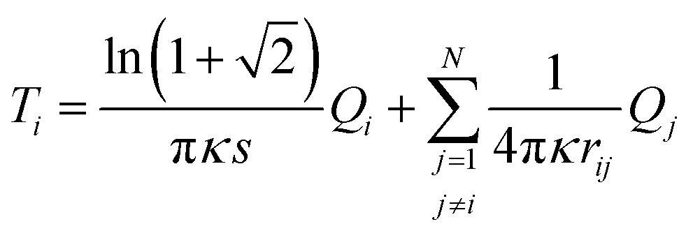
Let us consider a planar interface separating a solid substrate and a surrounding medium (typically a liquid). This interface features a heat source density (HSD, power per unit surface) q(r) over a limited domain![[scr D, script letter D]](https://www.rsc.org/images/entities/char_e523.gif) . This HSD is responsible for a temperature increase distribution T(r) everywhere in the system.
. This HSD is responsible for a temperature increase distribution T(r) everywhere in the system.
In this paragraph, we explain how one can numerically solve the inverse problem that consists in computing the heat source density q(r) required to produce a desired temperature field T(r) at the interface. Note that this procedure is not restricted to a 2D distribution. In principle, it could be applied to 3D temperature shaping, although a 3D heat source density would be difficult to realize experimentally. For this problem, we mesh the domain in N identical square unit cells of area s2. For each unit cell i, the temperature is named Ti and the delivered heat power Qi = s2qi. Ti can be simply expressed as a function of the Qi components:
 | (1) |
T = ![[Doublestruck A]](https://www.rsc.org/images/entities/i_char_e164.gif) Q Q | (2) |
is an N × N matrix such that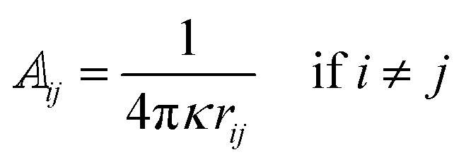 | (3) |
 | (4) |
Conversely, if a desired temperature distribution T is set, the associated heat source density can be obtained by inverting eqn (2):
| Q = −1T | (5) |
Hence, finding the appropriate heat source density only requires the inversion of the N × N matrix . As an example, if a uniform temperature increase T0 is desired over , each unit cell i has to deliver a heat power:
 | (6) |
This theoretical approach is illustrated in Fig. 1, which presents numerical simulations of arbitrarily shaped heat source densities and the associated temperature distributions. For the sake of clarity, a reduced number of cells (27) were used. Fig. 1a and b illustrate that a uniform HSD is far from giving a uniform temperature distribution. In contrast, Fig. 1c and d show how the inversion of the matrix can lead to the determination of the heat source density required to produce a uniform temperature profile over .
 | ||
| Fig. 1 Illustration of the theoretical procedure. (a) Uniform heat source density over the domain composed of N unit cells (N = 27 in this example). (b) Associated calculated temperature distribution obtained by multiplication with the N × N matrix . (c) Calculated heat source density using the inversion algorithm aimed at establishing a desired temperature distribution over the domain of interest , here a uniform temperature, represented in (d). | ||
In order to illustrate the capabilities of the TSUNA technique, various examples of higher-resolution maps are presented in Fig. 2. Fig. 2a presents the temperature distribution obtained when a circular area is uniformly heated. Note that the temperature is clearly non-uniform over the heated area. Fig. 2b presents a calculated HSD that was designed to create a uniform temperature distribution. The HSD naturally features higher values at its boundaries. Comparing Fig. 2a and b gives an idea of the benefit of using structured HSD distributions to shape a temperature profile. Note that using the TSUNA technique, the temperature is supposed to be controlled only within (i.e. the area that delivers heat). Indeed, outside the temperature is no longer controlled and decays in 1/r (r being the radial coordinate). Fig. 2c–e represent other geometries featuring a uniform temperature distribution. It can be shown that the TSNUA approach can lead to uniform temperature distributions of any geometries. Shaping a uniform temperature distribution is not the only capability of the TSUNA technique, Fig. 2f presents a HSD that was designed to create a linear temperature gradient over a rectangular area. More sophisticated temperature profiles can be achieved, such as a parabolic profile (Fig. 2g) or temperature profiles over disconnected domains, as represented in Fig. 2h and i.
 | ||
| Fig. 2 Numerical simulations of various HSDs and the associated temperature distributions. A horizontal cross-cut in the middle of the image is represented for each map. No scale bars are displayed since the simulations are not scale dependent (i.e. the same profiles would be observed regardless of the size of the system). (a) The case of a uniform heat source density. (b–e) Heat source densities of various shapes aimed at creating uniform temperature distributions. (f) HSD that creates a linear temperature gradient. (g) HSD that creates a parabolic temperature distribution. (h) HSD that creates a uniform temperature profile over a disconnected area. (i) HSD that creates an asymmetric two-temperature dimer. (j) Two-temperature dimer structure where the HSD features some negative values. | ||
Finally, Fig. 2j addresses a limitation of the TSUNA technique that is worth discussing. Of course, any temperature distribution cannot be designed using realistic HSDs. Temperature is firstly governed by the Poisson equation, which imposes some constraints. The inversion algorithm always gives a HSD distribution for any temperature map, but if some inappropriate temperature distributions are entered in the algorithm, the direct consequence will be a computed HSD image featuring some negative values in some pixels. Such an issue is visible in the HSD cross-cut in Fig. 2j. The temperature gradient imposed between the two discs is stronger that the natural 1/r decay of the temperature profile. The consequence is the presence of a negative HSD at the dimer gap location, which means the presence of a heat sink (not a heat source), unfeasible experimentally using the TSUNA technique. Another typical prohibitive case is a temperature distribution featuring a zero value somewhere over . This is understandable since as soon as at least one HSD pixel is not zero, heat is delivered in the system and the temperature is no longer zero at any place in the system. Hence, one needs to keep some physical insight when designing desired temperature distributions.
2.2 Sample design
Experimentally, the challenge consists in fabricating a distribution of absorbing NPs faithfully reproducing (when illuminated) the calculated HSDs, such as the ones represented in Fig. 2. Under illumination, a metal NP absorbs part of the incoming light, which contributes to heat the NP and turn it into an ideal nanosource of heat remotely controllable by light.24,25 The use of metal NPs as nanosources of heat is a promising approach to investigate temperature triggered processes on the nanoscale in recent areas of research such as nanochemistry, thermal biology or microfluidics. For this purpose, metal NPs made of gold are usually preferred since they feature enhanced optical absorption in the visible-infrared range due to plasmonic resonances.26The strategy we propose herein consists in fabricating by e-beam lithography an assembly of close-packed identical NPs with a NP density that spatially varies according to the calculated HSD map. The procedure to produce an appropriate NP position list is detailed in Fig. 3. The first step consists in smoothing the HSD map to avoid sharp spatial variations from one pixel to another, especially around the boundaries (Fig. 3b). Smoothing is not necessary, but recommended. If the meshing is fine enough, smoothing the HSD does not affect the overall shape of the desired temperature. It just smoothes the final temperature profile around the edges of the domain . Then, the basic idea is to replace each pixel j ∈ N of the smoothed HSD map by a set of nj NPs proportional to the HSD value Qj. The HSD map should be re-coded over a scale of integers ranging from 0 to Nmax (Fig. 3c), representing the number of NPs, where Nmax is the maximum number of NPs that can fit within a unit cell area of the sample (UCAS). There is some freedom regarding the choice of Nmax. A low value of Nmax permits the design of smaller structures, but the HSD will be more poorly coded, and reciprocally for a large value of Nmax. Nmax = 16 or 25 seems a good compromise. In the particular case of Fig. 3c, Nmax = 25. In order to evenly fill each UCAS with nj NPs, a set of Nmax patterns has to be previously tidily designed, representing the NP positions in a UCAS for each possible value of nj. Two sets of patterns corresponding to Nmax = 16 and Nmax = 25 are provided in the ESI.† The (nj)j∈[1,N] maps, along with the Nmax patterns, are finally used to build a full NP position list as represented in Fig. 3d. The position list can be finally used to design the associated NP distribution using e-beam lithography. The simplest approach consists in fabricating nanodots that can be as small as 40 nm using a standard e-beam lithography device. Fig. 3e presents a Scanning Electron Microscope (SEM) image of a gold NP distribution designed using the position list represented in Fig. 3d. In this example, the NP smaller interdistance was set to 60 nm. In order to achieve smooth and continuous temperature distributions, despite of the discrete nature of the heat source density, a sufficient number of NPs along with a small NP interdistance have to be ensured.23
 | ||
| Fig. 3 Successive steps of the procedure aimed at reproducing experimentally the calculated heat source density. (a) Calculated heat source density. (b) Smoothed heat source density. (c) Converted smoothed heat source density using a 25-level scale. (d) Associated NP position map. (e) SEM image of the fabricated sample of gold NPs. | ||
2.3 Experiments
In order to illustrate the TSUNA procedure, we performed thermal measurements on gold nanoparticle samples obtained using the procedure described above. NP position lists such as the one presented in Fig. 3e were generated using Matlab from the inversion algorithm as gray scale bmp files. These files were then directly used in the e-beam lithography software (Elphy) to set the NP locations. The sample was baked at 200 °C in order to make the gold NPs spherical and to center the plasmonic resonance around 530 nm. This way, we obtained nanoparticles 40 nm in diameter. The HSD images were coded over Nmax = 25 values with a minimal NP interdistance of 100 nm. Some freedom exists regarding the choice of the nanoparticle interdistance. However, in order to keep the heat delivery proportional to the density of nanoparticles, optical coupling has to be avoided. Numerical simulations on a gold dimer using the boundary element method27 show that as far as the gap between two spherical nanoparticles is not smaller than the nanoparticle radius, no coupling occurs (see ESI†). In the experiments reported herein, the smaller gap between neighboring nanoparticles (60 nm) is three times larger than the nanoparticle radius (20 nm), which ensures no coupling effect.Optical heating of the NPs was performed using a wide field laser illumination at λ = 532 nm (see ref. 13 for a detailed description of the experimental setup). The thermal measurements were performed using a microscopy technique we recently developed and we named it TIQSI for Thermal Imaging using Quadriwave Shearing Interferometry (see the Methods section).22 This technique enables both mapping of the temperature and the heat source density (power per unit area) on the substrate surface, where the NPs are located. Briefly, using this technique, a plane optical wavefront crosses the region of interest and undergoes a distortion due to the thermally-induced variation of the refractive index of the medium (glycerol in our case). This wavefront distortion is imaged quantitatively using a QSI wavefront analyzer. The source was a collimated light emitted diode whose emitting spectrum spans from 600 nm to 650 nm (Thorlabs, M625L2-C1). The QSI wavefront analyzer was purchased from Phasics SA Company (Sid4Bio camera). Each image presented in this work is the result of the average of 50 wavefront images, corresponding to a whole acquisition time of around 5 seconds.
Fig. 4 presents the results obtained on a set of six different NP distributions. SEM images of the sample are provided in the ESI.†Fig. 4a and b represent measured HSDs arising from NP distributions aimed at creating a uniform temperature profile. The associated measured temperature profiles are represented in Fig. 4g and h and feature as expected a uniform temperature over a square area. Fig. 4a and g are meant to be compared with Fig. 4d and j, which corresponds to a uniform NP distribution of the same geometry. While the temperature represented in Fig. 4g equals 46.1 ± 0.5 °C on the heated area, it equals 51.2 ± 3.3 °C in Fig. 4j. Note that 0.5 °C is precisely the uncertainty of our temperature measurement, which suggests that the actual temperature distribution could be even more uniform than what we measure. Then, the weak standard deviation of the temperature increase achieved on the heated area in Fig. 4a compared to Fig. 4d illustrates the gain of our approach. Fig. 4c and i illustrate the possibility of generating a linear temperature gradient over a rectangular domain. Fig. 4e and k illustrate the possibility of generating a parabolic temperature profile and Fig. 4f and l an asymmetric temperature distribution.
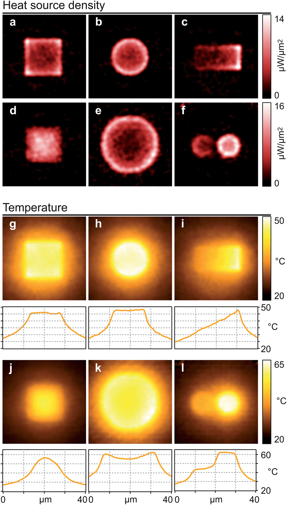 | ||
| Fig. 4 Thermal measurements on various gold NP patterns. (a–f) TIQSI measurement of the heat source density delivered by gold nanoparticle assemblies. (g–l) TIQSI measurement of the associated temperature distributions along with horizontal crosscuts. | ||
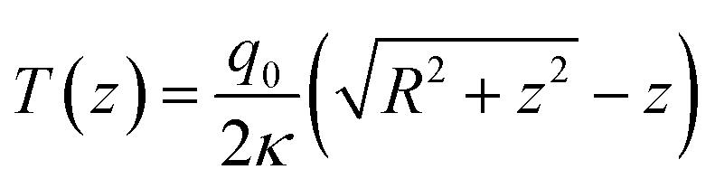
A feature of the temperature profile that is worth discussing in the context of this work is the actual three-dimensional temperature distribution further from the glass/liquid interface obtained with our approach. Since no heat delivery is performed out of the z = 0 plane, a natural 1/z decrease of the temperature is expected along the z direction far from the heat sources. More precisely, we can have a good estimation of the z profile for any nanoparticle distribution by considering a uniform and circular heat source density, of radius R. In this case, the temperature profile along the z direction from the centre of the distribution reads:
 | (7) |
The derivation of this equation is provided in the ESI.† From this equation, we can express the temperature decrease as a percentage compared to the maximum temperature at the centre of the distribution:
 | (8) |
This expression is close to 1 − z/R for small values of z/R, which allows for a simple estimation of the temperature decrease in z. For instance, T(z) will remain above α = 90% of the desired value if z < R/10. Shaping a temperature field in three dimensions would require a heat source distribution in three dimensions, which is not easily feasible, especially upon working in liquid. However, most of the envisioned applications will not suffer from this decrease in z. Indeed, observing processes at the microscale (especially using our optical approach) usually involves a microscopic objective, whose depth of field will not exceed one micrometer anyway. Hence, the temperature higher in the liquid will be related to a volume out of the domain of interest in the sample. Moreover, if we think about applications in biology, a living cell in culture is an object that is much wider than thick: around 15 micrometers in diameter and around 1 micrometer thick, except at the nucleus location. Hence, the temperature will be the one dictated by our technique within the cell volume, according to eqn (8). The same reasoning would apply for nanochemistry experiments were chemical reactions would be monitored at the focus plane of the objective.
Interestingly, two other strategies to shape a HSD at small scales may be considered. First, instead of varying the NP density, one could vary the NP morphology from one pixel to another of the HSD map. Such an approach would lead to temperature profiles controlled over much reduced spatial scales since only one nanostructure will be associated with each HSD pixel. However, a calibration relating the NP morphology and the absorption cross-section would have to be priorly determined. Another approach could consist in illuminating a uniform NP distribution with a structured laser illumination reproducing the HSD. The benefit of this approach would be the possibility to dynamically modify the HSD from the far field and it would not require an e-beam lithography process. However, the HSD spatial resolution will be diffraction limited, which will lead to much larger heated areas and a poorer spatial resolution. The approach we propose in this work, based on the use of contrasted NP distributions, cumulates the advantages of high resolution and simplicity.
3 Conclusion
In summary, we propose a numerical algorithm, along with an experimental procedure, intended to shape at will temperature distributions at the microscale. The numerical algorithm computes the heat source density required to produce a desired temperature distribution and e-beam lithography is used to design non-uniform gold nanoparticle distributions that mimic the heat source density. We illustrate the experimental feasibility of the procedure by carrying out measurements of the heat source density and the temperature over various NP distributions.Achieving controlled temperature distributions on the nanoscale appears valuable for various applications. In particular, we envision promising applications in cellular biology or nanochemistry. Indeed, some recent studies evidenced the significance of gold nanoparticles as a nanosource of heat in these areas of research. As explained above, illuminating an assembly of gold NPs is not supposed to yield a uniform temperature distribution, which could be problematic since a precise temperature control is often required in biology or chemistry. For instance, one could think of studying single cells on gold NP patterns aimed at creating a uniform temperature increase, such as in Fig. 4h. This would ensure the cell to undergo a uniform, albeit localized, temperature increase. Creating asymmetric temperature profiles such as the one presented in Fig. 4l could even lead to different temperature increases in different compartments of a cell. Creating a uniform temperature gradient could be also handy to evidence at a glance what the temperature threshold is for a given chemical transformation on the microscale. More generally, since any area of science features thermally induced effects, the ability to spatially control a temperature distribution on the microscale should enable the study of thermal induced microscale effects in a wide variety of areas of research.
Acknowledgements
The authors acknowledge financial support from research French agency ANR grant Tkinet (ANR 2011 BSV5 019 05) and ANR Infrastructure networks grant France Bio Imaging (ANR-10-INSB-04-01). This work was also partially supported by the European Community's Seventh Framework Program under grant ERC-Plasmolight (259196), and Fundació privada CELLEX. EBU acknowledges the support of the FPI fellowship from the Spanish Ministry of Science and Innovation (MICINN).References
- C. W. Chang, D. Okawa, A. Majumdar and A. Zettl, Science, 2006, 314, 1121 CrossRef CAS PubMed.
- L. A. Wu and D. Segal, Phys. Rev. Lett., 2009, 102, 095503 CrossRef.
- L. Wang and B. Li, Phys. Rev. Lett., 2008, 101, 267203 CrossRef.
- L. Cao, D. Barsic, A. Guichard and M. Brongersma, Nano Lett., 2007, 7, 3523–3527 CrossRef CAS PubMed.
- G. Baffou and R. Quidant, Chem. Soc. Rev., 2014, 43, 3898–3907 RSC.
- M. Zhu, G. Baffou, N. Meyerbröker and J. Polleux, ACS Nano, 2012, 6, 7227–7233 CrossRef CAS PubMed.
- A. Heber, M. Selmke and F. Cichos, ACS Nano, 2014, 8, 1893–1898 CrossRef CAS PubMed.
- X. Serey, S. Mandal, Y. F. Chen and D. Erickson, Phys. Rev. Lett., 2012, 108, 048102 CrossRef.
- J. Donner, G. Baffou, D. McCloskey and R. Quidant, ACS Nano, 2011, 5, 5457–5462 CrossRef CAS PubMed.
- S. Duhr and D. Braun, PNAS, 2006, 103, 19678 CrossRef CAS PubMed.
- P. V. Ruijgrok, N. R. Verhart, P. Zijlstra, A. L. Tchebotareva and M. Orrit, Phys. Rev. Lett., 2011, 107, 037401 CrossRef CAS.
- D. Rings, R. Schachoff, M. Selmke, F. Cichos and K. Kroy, Phys. Rev. Lett., 2010, 105, 090604 CrossRef.
- G. Baffou, J. Polleux, H. Rigneault and S. Monneret, J. Phys. Chem. C, 2014, 118, 4890 CAS.
- D. Hühn, A. Govorov, P. Rivera Gil and W. J. Parak, Adv. Funct. Mater., 2012, 22, 294–303 CrossRef.
- A. S. Urban, M. Fedoruk, M. R. Horton, J. O. Rädler, F. D. Stefani and J. Feldmann, Nano Lett., 2009, 9, 2903–2908 CrossRef CAS PubMed.
- A. N. G. Parra-Vasquez, L. Oudjedi, L. Cognet and B. Lounis, J. Phys. Chem. Lett., 2012, 3, 1400–1403 CrossRef CAS.
- G. Baffou and H. Rigneault, Phys. Rev. B: Condens. Matter Mater. Phys., 2011, 84, 035415 CrossRef.
- G. Volpe, G. Molina-Terriza and R. Quidant, Phys. Rev. Lett., 2010, 105, 216802 CrossRef.
- T. Feichtner, O. Selig, M. Kiunke and B. Hecht, Phys. Rev. Lett., 2012, 109, 127701 CrossRef.
- B. Gjonaj, J. Aulbach, P. M. Johnson, A. P. Mosk, L. Kuipers and A. Lagendijk, Nat. Photonics, 2011, 5, 360–363 CrossRef CAS.
- B. Gjonaj, J. Aulbach, P. M. Johnson, A. P. Mosk, L. Kuipers and A. Lagendijk, Phys. Rev. Lett., 2013, 110, 266804 CrossRef CAS.
- G. Baffou, P. Bon, J. Savatier, J. Polleux, M. Zhu, M. Merlin, H. Rigneault and S. Monneret, ACS Nano, 2012, 6, 2452–2458 CrossRef CAS PubMed.
- G. Baffou, P. Berto, E. Bermúdez Ureña, R. Quidant, S. Monneret, J. Polleux and H. Rigneault, ACS Nano, 2013, 7, 6478–6488 CrossRef CAS PubMed.
- A. O. Govorov and H. H. Richardson, Nano Today, 2007, 2, 30 CrossRef.
- G. Baffou and R. Quidant, Laser Photonics Rev., 2013, 7, 171–187 CrossRef CAS.
- P. K. Jain, K. S. Lee, I. H. El-Sayed and M. A. El-Sayed, J. Phys. Chem. B, 2006, 110, 7238–7248 CrossRef CAS PubMed.
- U. Hohenester and A. Trügler, Comput. Phys. Commun., 2012, 183, 370–381 CrossRef CAS PubMed.
Footnote |
| † Electronic supplementary information (ESI) available. See DOI: 10.1039/c4nr01644k |
| This journal is © The Royal Society of Chemistry 2014 |