The equilibrium velocity of spherical particles in rectangular microfluidic channels for size measurement

Abstract

According to the Segré–Silberberg effect, spherical particles migrate to a lateral equilibrium position in parabolic flow profiles. Here, for the first time, the corresponding equilibrium velocity is studied experimentally for micro particles in channels with rectangular cross section. Micro channels are fabricated in PMMA substrate based on a hot embossing process. To measure individual particle velocities at very high precision, the technique of spatially modulated emission is applied. It is found that the equilibrium velocity is size-dependent and the method offers a new way to measure particle size in microfluidic systems. The method is of particular interest for microfluidic flow cytometry as it delivers an alternative to the scatter signal for cell size determination.

---

Introduction

Particles in laminar flow profiles (Poiseuille flow) are exposed to the inertial and viscous force which can move them perpendicular to the streamlines (inertial migration). For an initially uniform distribution of particles in suspension, Fåhreus¹ supposed in 1928 the development of a non-uniform distribution over the cross section of a circular tube after having travelled a certain distance at constant flow rate. The travelling distance is nowadays called “focusing length”. Furthermore, for a low particle concentration (4 # cm⁻³), where particle–particle interactions can be neglected, Segré and Silberberg demonstrated in 1961^2,3 that particles move to an equilibrium distance from the axis of a circular tube under certain flow conditions (“tubular pinch effect”). They found an equilibrium distance from the tube axis of approx. 0.6 of the tube radius. Recent experimental work in microfluidic channels performed by Hur et al.⁴ revealed a dependency between equilibrium position and particle diameter.

Over the last five decades a large number of experimental and theoretical studies have been conducted to understand the inertial migration of particles and to find the equilibrium position in different regimes of Reynolds numbers, various channel cross sections and flow profiles.^5–22 Based on the work of Saffman, 1965, and the work of Cox and Brenner, 1968, Ho and Leal derived in 1974 an expression for the lateral velocity of particles as well as for the streamwise velocity. They suggested particle trajectories describing the dynamics to reach equilibrium positions. Until today, all theories have been restricted to small ratios of particle size to channel height and low channel Reynolds numbers. A comprehensive predictive model for the size dependence of the equilibrium position is not available.

In the field of microfluidics, inertial migration is primarily studied for particle separation and filtration. The focus is on selecting the fluidic conditions such that particles of different size move towards different equilibrium positions.^23–26 A notable review of the field discussing the physics as well as prevailing applications was published by Di Carlo.²⁷

Obviously, under laminar flow conditions, the equilibrium position of a particle must be associated with a corresponding equilibrium velocity in flow direction. Almost all experimental studies mentioned, focus on the equilibrium position in a channel or tube with exception of Di Carlo et al.²⁸ in 2009. However, Di Carlo et al. do not report a significant correlation of equilibrium velocity and particle size. In this paper the fundamental question of the dependence between the equilibrium velocity and the diameter of the particle is experimentally addressed. A clear correlation is demonstrated and this finding enables the measurement of particle size solely based on particle velocimetry under controlled flow conditions.

Velocimetry of particles is mainly used to probe the flow profile (e.g. objects in the wind tunnel, microfluidic channel cross section etc.) by means of particle imaging velocimetry (PIV).²⁹ For these applications it has to be assured that the particles do not change the flow profile under investigation. This is primarily achieved by using particles which are several orders of magnitude smaller than the smallest dimension of the fluidic structure under investigation. In this field many different techniques for measuring the velocity of particles have been developed. For example, Gai et al.³⁰ have used the single molecule detection technique which is based on the use of an electron multiplier CCD camera for velocimetry of particles and single molecules. The requirements in the work presented here differ significantly. Firstly, the size of the particles and the smallest dimension of the fluidic structure have to be comparable. Secondly, as a consequence, the particles significantly affect the flow profile in their proximity.

The technique used for velocimetry here is based on spatially modulated emission first reported by Baßler and Kiesel.^31,32 This technique is primarily suitable for miniaturized flow cytometry and it provides the velocity information of a particle as a “by-product” of the particle detection.

The technical implementation and the experimental conditions of the measurement are presented in the experimental section. The result and discussion section shows the size dependence of the equilibrium velocity of five monodisperse particle populations and demonstrates the precision, the reliability and the dynamic range of particle discrimination. The potential of the new approach for particle size measurements is discussed in comparison to standard microscopy and dynamic light scattering. Finally, the relevance of the findings for the simplification of miniaturized flow cytometry is explained.

Experimental

The experimental setup and the data interpretation shown in this paragraph are based on the spatially modulated emission technique.^31,32 In brief, the operation principle of this technique is as follows: particles/cells are tagged with a fluorescent dye and are passed through a micro channel in a fluidic chip. While flowing through the channel the particles/cells cross a detection zone where a laser beam excites the fluorescent dye. A spatially patterned shadow mask covers the detection area and shades off the fluorescence for defined particle/cell positions. As a consequence of the particle/cell movement, this causes a fluorescent signal which is modulated in time and is recorded by a detector. For the detection of particles in the recorded signal, cross–correlation of the signal with the expected modulation sequence is used.

The fluidic chip

The plastic chip, made of PMMA XT, constitutes the essential part of the experimental setup since it ensures stable fluidic conditions. It is fabricated using hot embossing. Lithographically structured silicon on an insulator (SOI) wafer is used as a mould insert in order to emboss the channel structure in the PMMA substrate. The silicon layer on the wafer specifies the channel height. By means of this hot embossing procedure, surfaces in optical quality can be achieved.

To fabricate a closed channel, the PMMA substrate with the embossed channel structure needs to be sealed with a PMMA foil of 250 μm in thickness. Conventional methods are based on solvents. However, such techniques are not applicable in our case since it is extremely difficult to precisely control the thickness of dissolved PMMA substrate. As a consequence, the channel depth cannot be controlled at the required depth of 12.0 μm. Moreover, solvent bonding degrades the surface quality with respect to the optical quality. Therefore, a sealing technique based on UV irradiation was applied.³³ In order to bond two surfaces (PMMA substrate, PMMA foil) onto each other, they are firstly irradiated with UV light, decreasing the glass transition temperature of PMMA in a thin surface layer of approx. 100 nm in depth depending on the UV penetration depth and the dose absorbed by the material. Subsequently, the irradiated surfaces of the PMMA foil and substrate are brought in intimate contact. Again, hot embossing is applied at a force of 4500 N and a sandwich temperature of 70 °C. At this temperature the UV treated surface layers are above the glass transition temperature and melt together. The bulk material of the PMMA foil and substrate stays solid to maintain the desired channel structure. This process yields highly accurate channel structures as shown in the cross section of Fig. 1. A nearly rectangular channel profile is obtained with a mean width of 477.0 μm and a mean height of about 12.0 μm at the middle of the cross section. Along the channel length of 7 cm the channel profile is constant within a small variation in width of ±3.3 μm and height of ±1.0 μm. Extending from the upper corners of the fluidic channel the interface between substrate and film is visible, indicating remaining structural imperfections. Tensions remain in the plastic chip after the hot embossing process. This can be seen by the slight curvature of the bottom of the channel (see Fig. 1) which leads to the variation of the channel height. Simulations have shown that the conversion factor between the maximal velocity of the flow profile at a height of 12.0 μm and the flow rate is 3.16.

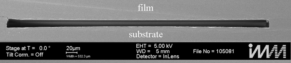Fig. 1 REM picture of the channel cross section in the fluidic chip. The cross section is nearly rectangular with a height of 12.0 μm and a width of 477.0 μm.

Fig. 2 shows a sketch of the fluidic chip in cross section (a) and top view (b). The hatched area in the cross section is the fluidic channel. Liquids enter the chip through the connectors 1, 2 and 3 and flow from right to left, leaving the chip through connector 4. Sample liquids are pumped through connector 1 at a flow rate of 8 μl min⁻¹. Sheath liquid (deionized water) is pumped in connectors 2 and 3 at a flow rate of 96 μl min⁻¹ for each connector. Under these flow conditions hydrodynamic focusing at the junction of the channels is realized and the sample flow is focused to a width of 20 μm (calculated with the theoretical model of Lee et al.³⁴). The reproducibility of the flow rates has been tested to be better than 0.5%. The parameters mentioned above lead to a Reynolds number of Re = 15 and an average velocity in the flow profile of <v> = 544 mm s⁻¹.

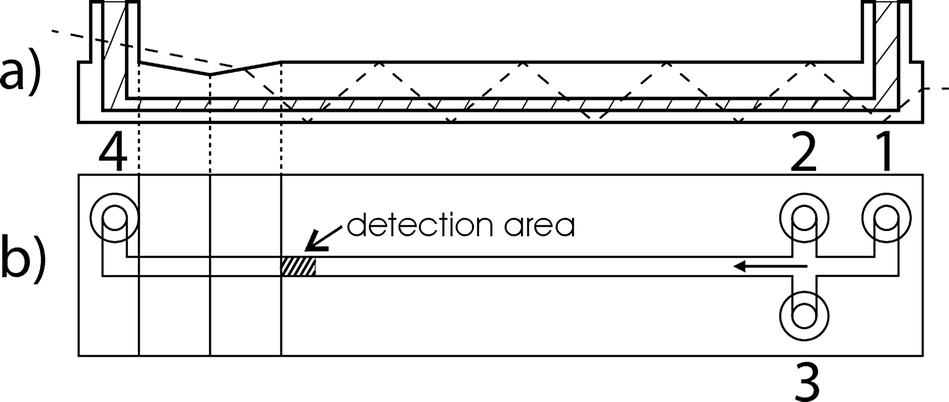Fig. 2 Sketch of the fluidic chip. a) Cross section of the chip along the channel. The hatched area is the channel. The dashed line shows the propagation of the excitation laser from left to right. b) Top view of the chip. The sample enters at port 1, port 2 and 3 are additional fluid inlets to establish hydrodynamic focusing at the junction of the channels. The arrow at the junction points in flow direction. The hatched area indicates the detection area. Port 4 is the outlet to the waste.

The sketched triangular groove in the top of the chip is required to couple in a laser beam (dashed line) for the fluorescence excitation of particles in the fluid (see below) at the detection area. The angle between the groove and the top of the chip is 10°. The configuration is chosen to couple the laser beam into the chip under the Brewster's angle which minimizes the reflection losses. Subsequently, the laser beam is guided through the chip by total internal reflection until it hits the escape surface at the right side of the chip.

Particles enter the detection area for fluorescent light at a distance of 47.5 mm from the centre of the channel junction. Since the fluorescent light of particles is isotropically radiated, a fraction escapes at the bottom of the chip where it is detected and processed (see below). Laser light which is scattered at surface imperfections, particles and edges can leave the bottom of the chip, too, and enter the detection optics. Hence, the chip is designed to minimize the propagation of laser light to the detector.

Experimental setup

Fig. 3 shows a sketch of the experimental setup. The laser beam emitted by the laser (a) (100 mW) is passed through an iris diaphragm (b) which absorbs scattered rays. The beam subsequently passes through a filter (c) (AHF Analysetechnik Laser Clean up Filter ZET 488/10×). The polarisation of the beam is then rotated into the plane of the optical table by a λ/2-plate (d). The laser beam is aligned at the Brewster angle enabling a reflection free refraction into the PMMA (n = 1.49) of the plastic chip (h) through the groove. The cylindrical lens (e) with a focal distance of 40 mm focuses the beam into the channel. The focal spot defines the excitation zone, which has a length of 2200 μm along and a width of 450 μm orthogonally to the channel.

Fig. 3 Sketch of the experimental setup. (a) 488 nm laser. The beam passes through an iris diaphragm (b), a laser clean-up filter (c), a λ/2-plate (d) and is focused into the channel of the plastic chip (h) by a cylindrical lens (e). The light emitted by the fluorescent particles is collected by a microscope lens (i) and subsequently passes through an optical filter (j). A microscope lens (k) identical to (i) focuses the fluorescent light on the spatially modulated mask (l). Subsequently the light is collected by a spherical lens (m) and focused onto the APD (n). A CMOS camera (f) and a spherical lens (g) are used for the alignment of the optical setup. The sheath and sample flow is supplied to the plastic chip by a syringe pump (o).

The fluorescently dyed polystyrene particles flowing in the channel are in the focal plane of the microscope lens (i) (Leitz 25×/NA 0.4; 569244), which collects and collimates the fluorescent light emitted by the particles. This is crucial in order to enable the optical interference filter (j) (AHF Analysetechnik BrightLine® HC 578/105) to work at its maximum performance. The filter transmission is from 506 nm to 594 nm blocking scattered excitation light and transmitting the fluorescent light which is collected by an inverse microscope lens (k), which is equivalent to (i). The fluorescent light is focused onto the spatially patterned shadow mask (l) (see also Fig. 4). In that way the fluorescent particles in the channel are imaged onto the mask. Behind the mask the light is collected by a spherical lens (m) (f = 20 mm) and is focused onto a single APD (SensL SPMini). The signal from the APD is continuously recorded. Consequently, for a fluorescent particle which moves through the channel the fluorescent light which reaches the APD is modulated by the mask, resulting in a temporally modulated output signal.

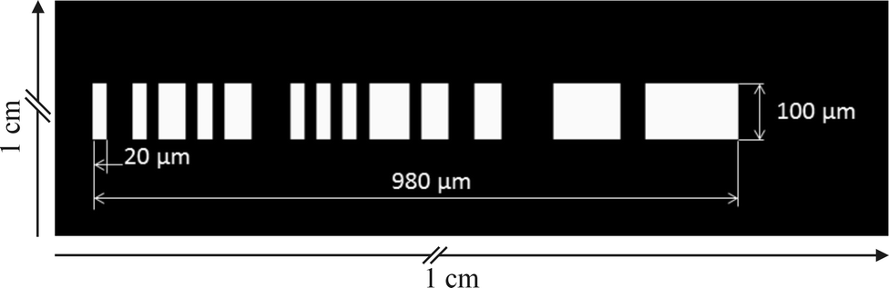Fig. 4 Sketch of the optical mask generated from the LABS 50. Each digit has a length of 20 μm; the total length is therefore 980 μm from the left edge of the first open feature (#1) to the right edge of the last open feature (#49). The very last feature (#50) is opaque and cannot be distinguished from the surrounding mask body.

The CMOS Camera (f) (Photonfocus MV-D1024E-160-CL-12) as well as the spherical lens (g) (f = 20 mm) are used for alignment purposes of the optical detection path.

The sample and sheath flow is supplied by a syringe pump (o) (Cetoni Nemesys MidPressure Modules).

Particle suspension

In order to demonstrate the ability to distinguish between populations by means of velocimetry, Fluoresbrite® Polychromatic (PC) Red Microspheres (diameter: 5.51 μm, Polysciences Inc.) and SPHERO™ Fluorescent Nile Red Particles (diameter: 0.84 μm, 2.11 μm, 3.30 μm, 4.24 μm and 6.42 μm, Spherotech Inc.) are used. All particles are made of polystyrene and are suspended in deionised water (18.2 MΩ cm). According to the manufacturer's specification, the size distribution for the 5.51 μm particles has a standard deviation of 0.122 μm. The excitation maxima of the Polychromatic Red dye in the microspheres are at 491 nm and at 512 nm; the emission maximum is at 554 nm (according to Polysciences Inc. specification). The excitation maximum for the Nile Red dye is at about 510 nm; the emission maximum is at about 555 nm. The mean fluorescent intensity of the particles is not unambiguously related to the mean particle diameter. In control experiments in our setup we therefore measured the mean fluorescent intensity to be 41.6 mV for the 6.42 μm population, 590.2 mV for the 5.51 μm population 11.0 mV the 4.24 μm population, 40.9 mV the 3.30 μm population, 13.3 mV for the 2.11 μm population, and 1.8 mV for the 0.84 μm population. Four different suspensions were prepared: all containing 5.51 μm and 0.84 μm particles which are used as control particles. In addition each suspension contains either 2.11 μm, 3.30 μm, 4.24 μm, or 6.42 μm particles. The total particle concentration is 5 × 10⁵ # ml⁻¹ and the share of each population is one third (1.66 × 10⁵ # ml⁻¹). Each suspension is passed through the experimental setup for a duration of 3 min and the fluorescent intensity as well as the velocity of each detected particle is measured.

Spatial mask

The spatial mask sketched in Fig. 4 and applied in the experimental setup follows a binary sequence with a length of 50. The sequence is [−1,1,−1,−1,1,−1,1,1,−1,1,−1,1,1,−1,−1,−1,1,−1,1,−1,1,−1,1,1,1,−1,1,1,−1,−1,1,1,−1,−1,−1,−1,1,1,1,1,1,−1,−1,1,1,1,1,1,1,1] and the physical representation is transparent for “1” and opaque for “−1”. The sequence is selected according to the theory of “low autocorrelation binary sequences” (LABS).³⁵ The key criterion for selecting an appropriate sequence is the main peak to maximum side lobe ratio (PSLR) calculated from the autocorrelation function of the sequence. Optimal sequences need to have minimal side lobes arising in the autocorrelation signal. Side lobes could be seen as an “intrinsic noise” of the sequence itself. Consequently, this “noise” should be as low as possible compared to the main correlation peak used for particle detection. For the selected LABS the PSLR is 12.12.

The smallest feature of the mask in our setup is set to 20 μm so that particles with a diameter as large as the channel height of 12 μm produce a fully modulated signal in the detector. The absolute length of the mask is set to 1000 μm which is well within the field of view of the microscope lens and the size of the excitation area ensuring homogeneous illumination throughout the particle passage. Since the rightmost digit of the chosen LABS 50 is −1 and thus opaque, the effective length of the mask is reduced to 980 μm.

The width of transparent mask features is 100 μm orthogonal to the channel axis which is well above the width of the hydrodynamically focused particle suspension (20 μm) to ensure signal modulation. The opaque area of the mask surrounding the transparent features (indicated by the black area in Fig. 4) is 10 × 10 mm and blocks any unwanted excitation light reflected from the channel walls, surface and material imperfections as well as from the particles.

Interpretation of the data

The signal of the APD is continuously sampled and digitized by the NI digitizer PCI-5922. Consider now a section of the signal S(t_i) at time step t_i with length N

S(t_i) = s_i+n = s_i+0, s_i+1, s_i+2⋯, s_i+N−1, n = 0, 1, 2, ⋯, N,

and a second sequence

F(v_k) = f_nk = f_0k, f_1k, f_2k, ⋯, f_N−1,k

representing an ideal signal of a particle with velocity ν_k passing the spatial mask of Fig. 4. This sequence is called filter F.

In order to identify a particle in S and its velocity, a set of K filters is calculated, each representing a velocity ν_k. Afterwards the cross–correlation of all K filters and signal S is calculated.

The result is a matrix of K correlation values for each time step. The low frequency components in the matrix are removed by means of a discrete wavelet transformation using the coiflet 5 wavelet³⁶ so the matrix is “detrended” and well prepared for peak detection based on a threshold operation as depicted in the 3D plot of Fig. 5.

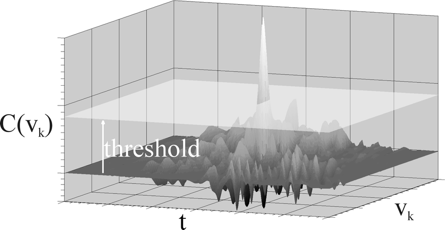Fig. 5 3D plot of the correlation matrix for a particle with 0.84 μm diameter. If a peak pierces through the threshold plane, a particle is detected. Position and amplitude of the maximum give intensity, velocity and time stamp for the particle.

As seen in Fig. 5, a threshold plane is used and every peak below this threshold is discarded as noise. A peak rising above the threshold identifies a particle. The maximum peak value gives the fluorescent intensity, the position of the maximum on the velocity axis gives the particle velocity and the position on the time axis gives a time stamp for the particle transition which is of no interest here.

Results and discussion

The scatter plot in Fig. 6 shows the fluorescent intensity as a function of velocity for all particles in each particle suspension. The 0.8 μm population exhibits by far the broadest velocity distribution (see inset in Fig. 6, a)). For the 0.8 μm particles, inertial migration is not developed and therefore these particles are broadly distributed over the channel height and can therefore be used to probe the flow profile. From the velocity distribution we determined the maximum in the flow profile by evaluating the cut-off velocity via a fit-routine. The results are listed in Table 1 and are plotted in Fig. 7 for all four measurements. The mean maximal velocity is 658 mm s⁻¹ and the measured variation of approximately 0.3% is ascribed solely to the reproducibility of the syringe pump. In an accompanying study the reproducibility of the flow rate of the syringe pump was determined to be better than 0.5%.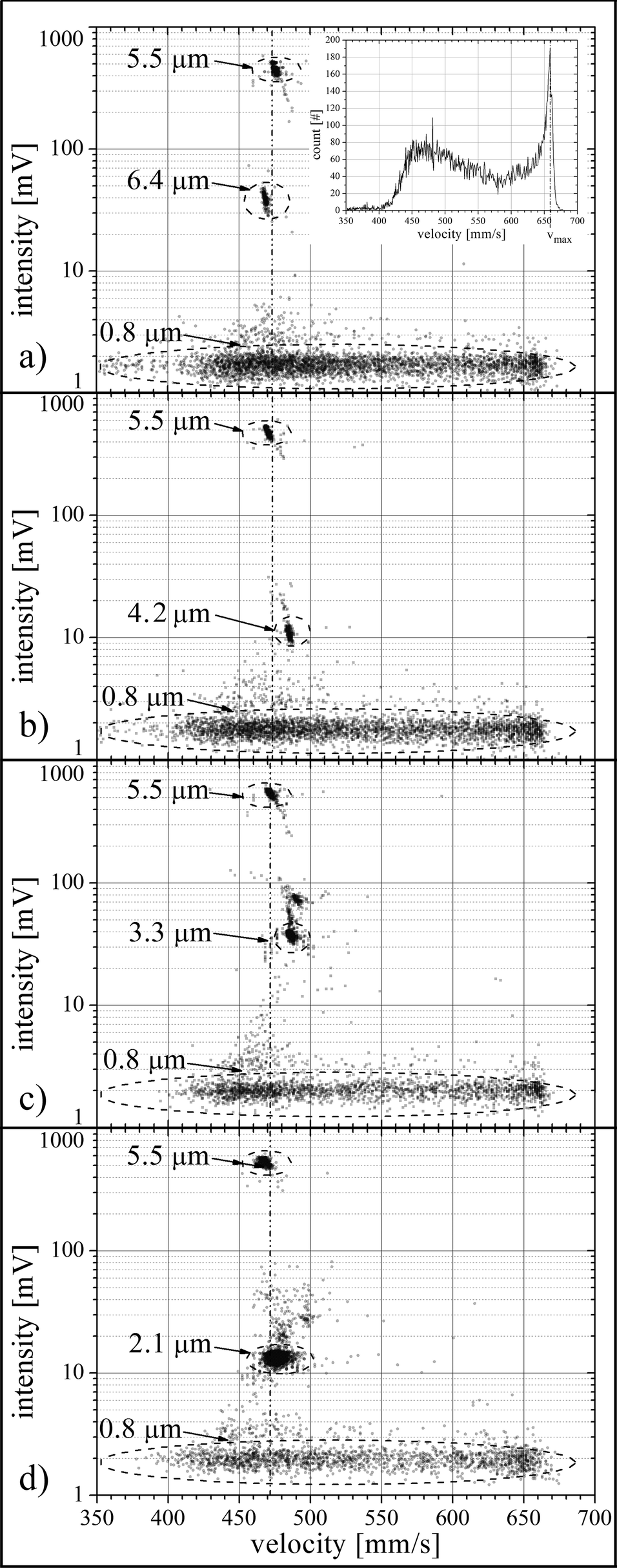

Fig. 6 Scatter plot for the all particle suspensions. Each data point represents the velocity and the fluorescent intensity of a detected particle. Clearly visible distinct particle populations (dashed ellipses) were attributed to the respective particle diameter by means of the fluorescent intensity.

Table 1 The results of the four different suspension measurements are summarized in the table. The values of the mean velocity are obtained by applying a Gaussian fit to the velocity distribution

	Mean particle diameter of population	Mean velocity	Maximum velocity	Standard deviation	Particle count
	μm	mm s^−1		mm s^−1	#
2.1 μm suspension measurement	0.8	—	658.1	5.6	1678
	2.1	482.9	—	3.1	2052
	5.5	473.1	—	2.4	265
3.3 μm suspension measurement	0.8	—	659.0	3.7	2111
	3.3	486.1	—	1.5	1277
	5.5	472.1	—	1.4	441
4.2 μm suspension measurement	0.8	—	658.1	4.1	3549
	4.2	485.3	—	1.1	315
	5.5	471.0	—	1.1	256
6.4 μm suspension measurement	0.8	—	656.9	5.1	3600
	6.4	468.9	—	1.4	324
	5.5	475.7	—	1.3	201

---

Fig. 7 The maximal velocity of the flow profile, measured by the use of 0.8 μm particles and the mean velocity of the 5.5 μm particles of every measurement is plotted against the daytime at which the measurement was started. The ambient temperature during day is also shown. The error bars of the data points are the standard errors of the mean.

The mean velocity of the 5.5 μm particle population is obtained by a Gaussian fit applied to the velocity distribution and is listed in Table 1 and plotted in Fig. 7. The velocity distributions are remarkably sharp with a standard deviation varying between 1.1 mm s⁻¹ and 2.4 mm s⁻¹. We attribute the sharp velocity distribution to particle transport on the Segré–Silberberg equilibrium position with an associated equilibrium velocity. The data reveal variation of the 5.5 μm particle mean velocity significantly higher than the variation in maximal velocity (see Fig. 7) of the flow profile and is not correlated to it. However, a comparison with the ambient temperature in the setup reveals a correlation with the temperature drift in the laboratory during the day. At 9:30 in the morning the ambient temperature is 22 °C. About noon it rises up to 24 °C and in the late afternoon the temperature drops down to 20 °C at 17:00. Since there was minor temperature drift around noon, the variation of the 5.5 μm particle mean velocity of the 11:30 and 14:50 measurements strictly follows the variation of the maximal velocity of the flow. In the late afternoon (17:00) the temperature effect is clearly visible. The maximal velocity decreases by 1 mm s⁻¹ and at the same time the 5.5 μm particle mean velocity rises by 4.5 mm s⁻¹. While the temperature goes down, the viscosity increases and thus the effect of inertial force on the particles decrease relative to the viscous force. Our result indicates that this effect shifts the mean velocity of particles in a Segré–Silberberg position closer to the maximal velocity. The same accounts for the measurement in the morning at 9:30. Please note that changes in viscosity have minor impact on the maximal velocity as the syringe pump enforces flow rate by adapting feed pressure. As a consequence of the above findings, detailed studies with deliberately controlled viscosity are under way to quantify the relationship between viscosity and equilibrium velocity. Due to the temperature drift the channel Reynolds number varies between 13.8 at 20 °C and 15.7 at 24 °C and we specify a mean value of Re ≈ 15 for our experiments.

In Fig. 6, d) the 0.8 μm population consists of 1678 particles, the 2.1 μm population consists of 2052 particles and the 5.5 μm population consists of 265 particles. Outside of the three main populations 505 events are detected. From the initial conditions a particle count of approx. 4000 per population and a total of 12 000 are expected. The particle loss is due to particle sedimentation in the supply tube which has a diameter of 100 μm and a length of 10 cm. The mean particle distance in the measurement channel was 15 mm (28 ms) which is approx. 15 times the length of the detection zone (980 μm) and more than three orders of magnitude larger than the minimum channel dimension (height, 12 μm). Therefore, particle coincidence in the detection zone perturbing intensity measurement as well as hydrodynamic –particle–particle interactions can be neglected. Control experiments do not yield significantly different scatter plots for concentrations up to 5-fold of the initial concentration. The particle count of measurements, a), b) and c) is similar, as shown in Table 1.

The data points outside of the marked populations in Fig. 6 are aggregates of two or more particles. Examples have been found by visual inspection of the suspensions under the microscope. This effect is most obvious in the scatter plots for the 0.8 μm particles: A faint second population appears at 3.6 mV which is approximately twice the intensity of the main 0.8 μm particle population.

The velocity of the 5.5 μm particles of measurement Fig. 6, c) has been arbitrarily chosen as a visual guideline in Fig. 6 indicated by the dashed and dotted line. The mean velocities of the 2.1 μm population, the 3.3 μm population, the 4.2 μm population and the 6.4 μm population are again obtained by applying Gaussian fits. The results together with the standard deviations are listed in Table 1.

The 6.4 μm population, the 5.5 μm population and the 4.2 μm population can be clearly distinguished by means of the measured velocity. The mean velocity of the 6.4 μm population is 468.9 mm s⁻¹ and thus slower than the 5.5 μm population with a mean velocity of 475.7 mm s⁻¹ and again slower than the mean velocity of the 4.2 μm population with 485.3 mm s⁻¹. The 4.2 μm population and the 3.3 μm population with a mean velocity of 486.1 mm s⁻¹ have nearly the same velocity and are not distinguishable by means of the velocity. For the 2.1 μm population with a mean velocity of 481.05 mm s⁻¹ the inertial migration towards the equilibrium position is not completed, as can be seen from the comparatively large standard deviation of 3.1 mm s⁻¹. To complete the inertial migration, either the channel Reynolds number or the focusing length must be increased.

As all measurements contained the 5.5 μm particles, their equilibrium velocity is used as reference to compensate for the deviations introduced by the temperature drift. To obtain the data in Fig. 8, the mean velocity of the 5.5 μm particles is subtracted from the mean velocity of the respective other particle populations in the measurement. The bars attached to the data points now indicate the standard deviation of the underlying velocity distribution. For particles smaller than 4 μm the distributions obviously overlap. Size measurement based on the velocity is not possible in that range.

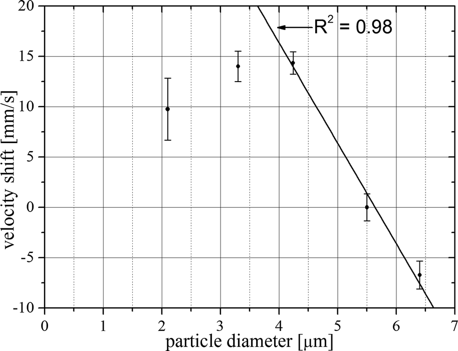Fig. 8 The velocity shift referenced to the mean velocity of each 5.5 μm population is plotted against every particle size. The bars attached to the data points are not error bars, these are the standard deviations determined by the Gaussian fit of every population and giving a feel for the selectivity.

In the range from 4.2 μm to 6.4 μm the relation between particle size and velocity is in first approximation linear as demonstrated by the regression line in Fig. 8. Please note again that the bars indicate the standard deviation of the velocity distribution. The width of each velocity distribution is a convolution of the error in determining the individual particle velocity (<0.1%) and the particle size distribution (unknown, see experimental section). The standard error in determining the mean value of the distribution is obtained by dividing the standard deviation by the square root of the particle count. The resulting error bars are smaller than the symbol size in Fig. 8 and are therefore omitted. In summary, Fig. 8 demonstrates that the equilibrium velocity of particles is well suited for size measurement under our experimental conditions. The limitations in resolution and dynamic range have not been studied so far. It is not known if an increased Reynolds number would shift the lower limit towards smaller particles. Please note that Di Carlo et al. (2009) did not find a significant correlation between equilibrium velocity and particle size under slightly different experimental conditions (Re = 20, channel height to particle size ratio: >0.4). This indicates the existence of a narrow window of experimental conditions for optimal size discrimination.

The prevailing particle size measurement methods are either dynamic light scattering or microscopy. Dynamic light scattering exploits the time response of optical scattering in particle suspensions. The method allows deriving the distribution of particle size based on the ensemble behaviour and performs best for monodisperse particle suspensions. The particle concentration needs to be low enough to keep the contribution of multiple photon scattering negligible. In case of polydisperse suspensions, the method becomes increasingly complicated as several scatter angles have to be measured and complicated mathematical models need to be applied for data evaluation. In contrast to dynamic light scattering, microscopy allows to measure individual particle sizes almost regardless of particle size. However, microscopy has generic limitations in gaining high statistics and high precision simultaneously. In the case of high precision, the optical field of view becomes small. In order to generate high statistics, the field of view needs to be scanned. In the case of a large field of view, the precision in size measurement is inevitably limited. In addition, microscopy gives very limited access to particle dimensions perpendicular to the optical plane.

Utilizing the propagation velocity, a purely hydrodynamic property of a particle governed by flow conditions offers several benefits. (1) The method is very fast and can easily process thousands of particles per second. Statistically significant data can thus be collected within a few seconds. (2) The size information is generated for each individual particle. Thus, particle sizes present in low concentration compared to other populations are not hidden due to statistical or signal intensity reasons. (3) Hydrodynamic forces and laminar flows can be precisely controlled and maintain their physical properties over a wide range of length scales. Thus, from micro particles down to nanoparticles the same physical regime governs the propagation velocity. Size ranges are not distinct due to various physical regimes such as in the case of the photon–particle interaction. Utilizing velocimetry for particle size measurement, however, requires a means for precise velocity measurement. Besides fluorescence, this can be done by light scattering, absorption, impedance measurement or magnetic interactions.

Conclusions

As posed in the result and discussion section, hydrodynamic forces on micro particles in microfluidic channels can be utilized to discriminate particles by size based on the particle equilibrium velocity in flow direction. Here, we demonstrated the principle for spherical particles with a diameter of 2.1 μm, 3.3 μm, 4.2 μm, 5.5 μm and 6.4 μm in shallow microfluidic channels (height of 12 μm) at a Reynolds number of Re = 15. The results are promising with respect to sensitivity and accuracy. However, a number of questions arise from the initial results and will be the focus of our future work. It has not been investigated how the equilibrium velocity depends on shape and deformability of the particles as well as viscosity of the carrier liquid. Moreover, no optimal conditions have been identified with respect to channel cross section, fluid viscosity and “focusing length”.

Besides application of the concept for precise size measurements of micro particles and nanoparticles, our findings have impact on miniaturized flow cytometry based on spatially modulated emission which inherently measures fluorescent intensity and velocity of moving objects. Thus, if appropriate flow conditions are chosen, velocimetry can be directly used to quantify cell size. In conventional flow cytometry additional detectors are required to measure a side and forward scatter to assess cell size.

This work also contributes to answering the fundamental question of the relation between particle size, equilibrium velocity and equilibrium position in the flow. In combination with the experimental results of Hur et al.⁴ on the connection of particle size and equilibrium position, the equilibrium velocity is a key parameter to validate theoretical models. However, little is known about one remaining open parameter: the angular velocity of a particle under equilibrium conditions.

Acknowledgements

The authors thank Tobias Broger who realized an extremely reliable and fail-safe data sampling system and Stefan Schmitt whose knowledge in silicon-based thin-film technology was key to fabricating precise microfluidic channels. We also thank Jörn Wittek and Karen Böhling for proofreading the text. The European Research Council (ERC) is acknowledged for funding the project under grant #258604.

Notes and references

1. R. Fahreus, Klin. Wochenschr., 1928, 7, 100–106.
2. G. Segré and A. Silberberg, Nature, 1961, 189, 209–210.
3. G. Segré and A. Silberberg, J. Fluid Mech., 1962, 14, 136.
4. S. C. Hur, N. K. Henderson-MacLennan, E. R. B. McCabe and D. Di Carlo, Lab Chip, 2011, 11, 912.
5. E. S. Asmolov, J. Fluid Mech., 1999, 381, 63–87.
6. F. P. Bretherton, J. Fluid Mech., 1962, 14, 284.
7. R. Cox and H. Brenner, Chem. Eng. Sci., 1968, 23, 147–173.
8. B. P. Ho and L. G. Leal, J. Fluid Mech., 1974, 65, 365.
9. A. J. Hogg, J. Fluid Mech., 1994, 272, 285.
10. J. B. McLaughlin, J. Fluid Mech., 1993, 246, 249.
11. R. V. Repetti and E. F. Leonard, Nature, 1964, 203, 1346–1348.
12. P. G. Saffman, J. Fluid Mech., 1965, 22, 385.
13. J. A. Schonberg and E. J. Hinch, J. Fluid Mech., 1989, 203, 517.
14. P. Vasseur and R. G. Cox, J. Fluid Mech., 1976, 78, 385.
15. L. Zeng, S. Balachandar and P. Fischer, J. Fluid Mech., 2005, 536, 1–25.
16. B. Chun and A. J. C. Ladd, Phys. Fluids, 2006, 18, 31704.
17. R. Eichhorn and S. Small, J. Fluid Mech., 1964, 20, 513.
18. K. J. Humphry, P. M. Kulkarni, D. A. Weitz, J. F. Morris and H. A. Stone, Phys. Fluids, 2010, 22, 81703.
19. R. C. Jeffrey and J. R. A. Pearson, J. Fluid Mech., 1965, 22, 721.
20. J.-P. Matas, J. F. Morris and É. Guazzelli, J. Fluid Mech., 1999, 515, 171–195.
21. D. R. Oliver, Nature, 1962, 194, 1269–1271.
22. J. Zhou and I. Papautsky, Lab Chip, 2013, 13, 1121.
23. T. E. Kagalwala, J. Zhou and I. Papautsky, in The 14th international conference on miniaturized systems for chemistry and life sciences. The proceedings of microtas 2010 conference, Chemical & Biological Microsystems Society, San Diego CA, 2010.
24. D. R. Gossett, W. M. Weaver, A. J. Mach, S. C. Hur, H. T. K. Tse, W. Lee, H. Amini and D. Di Carlo, Anal. Bioanal. Chem., 2010, 397, 3249–3267.
25. A. A. S. Bhagat, S. S. Kuntaegowdanahalli and I. Papautsky, Lab Chip, 2008, 8, 1906.
26. A. A. S. Bhagat, S. S. Kuntaegowdanahalli and I. Papautsky, Microfluid. Nanofluid., 2009, 7, 217–226.
27. D. Di Carlo, Lab Chip, 2009, 9, 3038.
28. D. Di Carlo, J. F. Edd, K. J. Humphry, H. A. Stone and M. Toner, Phys. Rev. Lett., 2009, 102, 094503.
29. R. J. Adrian, Annu. Rev. Fluid Mech., 1991, 23, 261–304.
30. H. Gai, Y. Li, Z. Silber-Li, Y. Ma and B. Lin, Lab Chip, 2005, 5, 443.
31. M. Baβler, P. Kiesel, O. Schmidt and N. Johnson, 2008, US 2008/0181827 A1.
32. P. Kiesel, M. Baβler, M. Beck and N. Johnson, Appl. Phys. Lett., 2009, 94, 41107.
33. R. Truckenmüller, P. Henzi, D. Herrmann, V. Saile and W. Schomburg, Microsyst. Technol., 2004, 10, 372–374.
34. G. B. Lee, C. C. Chang, S. B. Huang and R. J. Yang, J. Micromech. Microeng., 2006, 16, 1024–1032.
35. S. Mertens, J. Phys. A: Math. Gen., 1996, 29, L473.
36. P. S. Addison, The illustrated wavelet transform handbook, Introductory theory and applications in science, engineering, medicine, and finance, Institute of Physics Pub., Bristol, UK, Philadelphia, 2002.

---