Silicone passive equilibrium samplers as ‘chemometers’ in eels and sediments of a Swedish lake

Abstract

Passive equilibrium samplers deployed in two or more media of a system and allowed to come to equilibrium can be viewed as ‘chemometers’ that reflect the difference in chemical activities of contaminants between the media. We applied silicone-based equilibrium samplers to measure relative chemical activities of seven ‘indicator’ polychlorinated biphenyls (PCBs) and hexachlorobenzene in eels and sediments from a Swedish lake. Chemical concentrations in eels and sediments were also measured using exhaustive extraction methods. Lipid-normalized concentrations in eels were higher than organic carbon-normalized concentrations in sediments, with biota–sediment accumulation factors (BSAFs) of five PCBs ranging from 2.7 to 12.7. In contrast, chemical activities of the same pollutants inferred by passive sampling were 3.5 to 31.3 times lower in eels than in sediments. The apparent contradiction between BSAFs and activity ratios is consistent with the sorptive capacity of lipids exceeding that of sediment organic carbon from this ecosystem by up to 50-fold. Factors that may contribute to the elevated activity in sediments are discussed, including slower response of sediments than water to reduced emissions, sediment diagenesis and sorption to phytoplankton. The ‘chemometer’ approach has the potential to become a powerful tool to study the thermodynamic controls on persistent organic chemicals in the environment and should be extended to other environmental compartments.

---

Environmental impact

Equilibrium sampling with silicone ‘chemometers’ was applied to determine ratios of chemical activities in eels and sediments for polychlorinated biphenyls (PCBs) and hexachlorobenzene. The study was conducted in an isolated Swedish lake with background contamination and eels introduced in 1979. The chemical activities of the PCBs were lower in the eels than in the sediments (i.e., a_Eel/a_Sediment < 1), whereas lipid-normalized concentrations of the eels exceeded organic carbon-normalized concentrations of the sediments (i.e., BSAF > 1). This apparent contradiction is explained by higher sorptive capacity of biota lipids compared to sediment organic carbon. The ‘chemometer’ approach provided novel, thermodynamically based insight into bioaccumulation and is highly promising for studying thermodynamic controls on persistent organic contaminants in a variety of systems.

1. Introduction

Bioaccumulation is the accumulation of a chemical in an organism by two processes: (i) bioconcentration, in which the chemical is absorbed from the surrounding environment through respiratory and dermal surfaces and (ii) biomagnification, in which the chemical is enriched from lower to higher trophic levels.¹ Bioconcentration and biomagnification can have a different impact on the levels of chemicals in aquatic biota relative to the thermodynamic equilibrium level. Bioconcentration of persistent, non-metabolizable chemicals from water or sediments into aquatic biota leads to chemical activities in biota approaching those in water or sediments if exposure is sufficiently long.² In contrast, due to the digestive action, the activity of chemicals in feed can increase in the gut, which in turn can result in absorption of the chemicals even when their activity is lower in the feed than in the organism.³

Metrics used to describe bioaccumulation⁴ include the bioconcentration, biomagnification and bioaccumulation factors, biota–sediment accumulation factors (BSAFs) and trophic magnification factors.⁵ Common to all these metrics is that bioaccumulation is assessed by comparison of measured concentrations of chemicals normalized to the lipid or organic carbon (OC) content of the matrix. The goal of the normalization procedures is to translate concentrations in different media into a common metric that can be compared. However, in this approach potential differences in the sorptive capacities of different lipids, and between lipids and OC are not accounted for, and other sorbing phases of potential importance, such as proteins in lean biota^6–8 and black carbon in sediments,⁹ are neglected.

Fugacity, the equivalent partial pressure of a chemical in the gas phase,¹⁰ has been proposed as a metric for comparing levels of contamination in different media, as described by Clark et al.¹¹ and further elaborated by Mayer et al.¹² Recently, fugacity ratios have been used as part of an integrative approach to study and understand bioaccumulation.⁴ A similar concept was proposed by Webster et al.¹³ in their equilibrium lipid partitioning (ELP) approach. Chemical activity, which quantifies the energetic state of a chemical that determines the potential for spontaneous physicochemical processes, such as diffusion,^14,15 is also closely related to fugacity (see Text S1 in the ESI† for additional details on the chemical activity concept). In a pioneering paper, Di Toro et al.¹⁶ explained the equilibrium partitioning from sediments to biota lipids on a chemical activity basis, and Mackay et al.¹⁷ recently suggested chemical activity as a unifying concept in the environmental assessment and management of chemicals. However, a general limitation on the application of all these concepts is that they often rely upon total concentration data that are transformed into fugacities, ELP concentrations or chemical activities by normalization. Thus, while providing useful conceptual frameworks, they have so far not helped to address the difficulties in choosing the correct normalization procedure.⁸ Direct measurements of chemical activity and related parameters, which can be achieved with novel equilibrium sampling techniques,^15,18 offer a solution.

Here, we explore the utility of such a direct empirical approach for assessing bioaccumulation, and, more generally, for assessing differences in chemical activity or fugacity between environmental media: measuring equilibrium partitioning concentrations in polymer-based passive samplers equilibrated with biota and sediments as a proxy of chemical activity or fugacity in these media. Comparing chemical concentrations in the polymer after equilibration with two or more environmental media is equivalent to comparing the chemical activities or fugacities between those media. We selected silicone polymers as the reference phase, and employed them essentially as ‘chemometers’.^12,19 Recent research has shown that silicone possesses unaltered sorptive properties even if immersed in complex matrices such as sediments and fish oil,²⁰ making it suitable for sampling of sediments and biota.

This study aimed to explore the ‘chemometer’ approach using eels and sediments from a Swedish lake as a case study. We equilibrated silicone-based passive equilibrium samplers in eels and sediments collected from the same lake, determined the concentrations of selected persistent organochlorines in the silicone, calculated activity ratios, and compared them to ‘classical’ BSAFs.

2. Experimental

2.1. Passive equilibrium sampling

Silicone reference phases were brought into contact with eels and sediments in separate experiments designed to achieve equilibrium partitioning. In both cases, passive equilibrium sampling approaches that have been previously validated were used. We selected European eel (Anguilla anguilla) for this study since it has a very high lipid content, and thus is ideally suited for the silicone in-tissue sampling method for lipid-rich biota developed by Jahnke et al.²¹ For sediments, silicone-coated glass jars were used, following another method developed by our research group.^19,22,23

In previous studies, equilibrium sampling of polychlorinated biphenyls (PCBs) was applied to sediments from a Finnish lake²³ and the Baltic Sea.¹⁹ The measured chemical concentrations in the silicone (C_{Sil, Sed}, see Table S1 in the ESI† for the most important abbreviations) were then transformed into concentrations in model lipids at thermodynamic equilibrium with the sediments (C_{Sed, Lip}) according to

C_{Sed, Lip} = C_{Sil, Sed} × K_Lip/Sil (1)

where K_Lip/Sil (ref. 24) is the lipid/silicone partition ratio (corrected for lipid uptake into the silicone, for details see ref. 24). C_{Sed, Lip} exceeded measurements of lipid-normalized concentrations in sediment-dwelling worms²³ and herring.¹⁹ These observations suggested lower chemical activities in the organisms relative to the sediments, but empirical data using passive equilibrium sampling in biota and sediments from the same ecosystem have so far been lacking. It was therefore particularly interesting within the present study to determine whether the ratios of chemical activity in eels and sediments at the study site would be <1 or whether biomagnification had led to elevated chemical activity in eels relative to the sediments (i.e. activity ratios > 1).

2.2. Study site

Our study site is Lake Ången (58°75'15° N, 17°18'31° E, Fig. 1), a small (2.4 km² area) and shallow (5 m average and 8.5 m maximum depth) Swedish lake with no known sources of PCBs and hexachlorobenzene (HCB) other than the atmosphere. The lake is connected to the Baltic Sea through a narrow 200 m long stream. In 1979, 4800 eels aged 3–8 years were transferred to Lake Ången as part of an experiment carried out by the Institute of Freshwater Research at the Swedish University of Agricultural Sciences. When they reach sexual maturity, the eels attempt to migrate out of the lake to spawn and are collected in an eel trap that blocks the stream leading to the Baltic Sea (Fig. 1).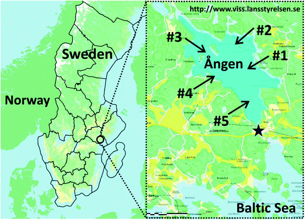

Fig. 1 Map of Lake Ången, Sweden. Sediment sampling was carried out at station #4 in 2011, and at stations #1 to #5 in 2012. The star shows the location of the eel trap in the connecting stream to the Baltic Sea.

2.3. Sampling

Samples of five eels that had been trapped in the stream leading towards the Baltic Sea were obtained from a local resident. One eel (“A”) was caught in the fall of 2011, whereas the other four individuals (“B” to “E”) had been trapped prior to 2011. For eels A–D a section of flesh from behind the gills was provided for chemical analysis, whereas for eel E a slice of muscle tissue from close to the caudal fin was provided. All five eels very likely originated from the stocking event in 1979 and hence had been present in Lake Ången for more than 20 years. The eels had been cut into sections and stored frozen since their capture, so length and weight information was not available for the five individuals that were used in our experiments. However, there are yearly monitoring data for the eels caught in the trap. Between 2002 and 2011, they were on average 104 ± 6 cm long and weighed 2220 ± 440 g.

Surface sediments were collected at site #4 (Fig. 1) by a diver on 19 November, 2011 by moving wide mouth glass jars over the sediment surface so that the upper 2–3 cm were transferred into the jars. The sediment was collected 20–30 m from a pier at Lomudden on the western shore of the lake at 2.5 m depth and 6 °C water temperature. The sediment samples were transported to the laboratory and stored at 4 °C until further processing. Additional sediment samples were collected at five sites across the lake (Fig. 1) using the same method on 24 November, 2012, at 3.6–7.0 m depth and 6 °C water temperature. The second sediment sampling campaign included the initial sampling location, station #4, to enable assessment of variability between the sampling campaigns.

2.4. Standards and materials

Seven indicator PCB congeners (PCBs 28, 52, 101, 118, 153, 138 and 180, log K_OW range 5.66–7.19 (ref. 25)) and HCB (log K_OW 5.64 (ref. 26)) were selected as model chemicals to evaluate our passive equilibrium sampling approach for bioaccumulation assessment. Isotope-labeled internal standard (IS) analogs were available for all the analytes (¹³C₆ HCB and ¹³C₁₂ PCBs). The IS analogs were spiked onto the sample or into the extraction solvent before extraction. Non-labeled PCB 53 was used as a volumetric standard and was spiked into the final extracts before analysis. All solvents and chemicals were of the highest available commercial quality and used as received.

Two different silicone polymers were used. Thin-films for eel sampling were cut from commercially available SSP-M823 sheets of approx. 30 × 30 cm size and 380 μm thickness (Specialty Silicone Products Inc., Ballston Spa, NY, USA). These films have a uniform thickness and hence the weight of each thin-film was also highly uniform. For sediment sampling, μm-thin layers of silicone were coated in-house on the inner vertical walls of 120 mL amber glass jars using a silicone (DC1-2577, Dow Corning, Seneffe, BE) solution in solvent. The amber glass jars were purchased from ApodanNordic PharmaPackaging A/S (Copenhagen, DK). The inner diameter of the jars was 5.5 cm, and the coating height was 4.6 cm, resulting in a surface area of the silicone coatings of 79 cm². The glass jar coatings were made from a different polymer than the one used in our previous work¹⁹ due to earlier problems with coating detachment during sediment sampling.

To account for differences in the sorptive properties of the two silicone polymers, compound-specific DC1-2577/SSP-M823 partition ratios (K_DC/SSP (ref. 27)) were applied. The polymers were inter-calibrated in co-exposure experiments, and K_DC/SSP were determined to be 1.70 (HCB), 2.11 (PCBs 101 and 153), 2.15 (PCB 28), 2.29 (PCB 180), 2.30 (PCB 118), 2.34 (PCB 52) and 2.65 (PCB 138) (on average 2.21).²⁷

2.5. Equilibrium sampling of eels

In-tissue sampling was done according to the method described in detail elsewhere.²¹ Briefly, circular thin-films of SSP-M823 silicone (18 mm in diameter) were precleaned in acetone and air-dried. Slots were cut through the eel skin using a scalpel, and the thin-films were immersed into the intact muscle tissue (n = 15 for each individual except for eel E, n = 12) for 2 days. During this time, the samples were wrapped in aluminum foil and stored at 4 °C in a refrigerator to slow down decay. The thin-films were then removed from the tissue, rinsed in double-distilled water, and their surface was thoroughly wiped using lint-free tissues to remove any tissue or fat remaining on the silicone surface. For each replicate (n = 3), 5 thin-films (4 for eel E) were pooled and immersed overnight at 21 °C in 10 mL acetone in a test tube with the IS (¹³C₆ labeled HCB and seven ¹³C₁₂ labeled PCBs, 10 μL of each solution at approx. 250 pg μL⁻¹ in toluene) added. In addition, 5 thin-films were extracted for each blank (n = 5). The solvent was then transferred to another test tube and exchanged to 1 mL isooctane before clean-up.

2.6. Equilibrium sampling of sediments

Passive equilibrium sampling of sediments was carried out using glass jars coated with DC1-2577 silicone of multiple thicknesses²² according to our published protocol.¹⁹ In brief, 80 g of wet sediment was added to a precleaned glass jar with a silicone coating of 2 μm, 4 μm or 8 μm (2011 samples, n = 3 for each coating thickness) or 1 μm, 2 μm or 4 μm (2012 samples, n = 1 per thickness). Jars with 10 mL of double-distilled water were processed as blanks (n = 3 for each coating thickness in 2011, n = 3 for the 1 μm jars in 2012). Approx. 100 mg of sodium azide was added to sample and blank jars to inhibit biological activity.

Each jar was covered with aluminum foil, sealed with the lid and rotated on its side at 21 °C for 2 weeks to allow for equilibration of HCB and the ‘indicator’ PCBs between the sediment and the silicone. The sediment was then discarded, the jar was rinsed twice with 2 mL aliquots of double-distilled water, and the silicone surface was thoroughly wiped with lint-free tissues. For extraction, 2 mL of acetone and 10 μL of each IS solution (see above) were added to the jar, and it was rotated on its side for an additional 30 min. The solvent was removed, and the extraction was repeated with another 2 mL aliquot of acetone. Both solvent aliquots were collected in a test tube and exchanged to 1 mL of isooctane before further processing.

2.7. Exhaustive extraction of eels and sediments

The total concentrations of the chemicals in muscle tissue of the five eels were determined by an exhaustive extraction method,²⁸ with modifications as previously described.²⁹ Briefly, 1 g of muscle homogenate (n = 3 for each individual) was extracted for 15 min in an ultrasonic bath with 4 mL of n-hexane : acetone (1 : 3) and the IS solutions (see above) added. The second extraction step used 4 mL of diethylether : n-hexane (1 : 9). The organic phases were combined and washed in 9 mL of sodium chloride : phosphoric acid (NaCl : H₃PO₄, 0.9% : 0.1 M). Afterwards, the organic phase was transferred to a preweighed pear-shaped flask and evaporated until a constant weight was observed. The dried residue was weighed to determine the extractable organic matter in the eels, before being reconstituted in 1 mL of isooctane for further processing as described below. Sediments were Soxhlet extracted with toluene and the IS solutions (see above) added as described by Bandh et al.³⁰ with some minor modifications.¹⁹ The extracts were evaporated before being reconstituted in 1 mL of isooctane.

The total organic carbon (TOC) content of the sediments was determined after homogenization and acidification to remove inorganic carbon using an elemental analyzer as described in ref. 19.

2.8. Common clean-up and analysis

All extracts were submitted to similar clean-up methods.²¹ The extract was pipetted onto a four-layered silica gel column (containing from bottom to top: glass wool, SiO₂ + water, SiO₂ + potassium hydroxide, SiO₂ + sulfuric acid and sodium sulfate, precleaned with n-hexane). The chemicals were eluted using n-hexane, and the extracts were concentrated to approx. 1 mL. In the case of total extracts of eels, two or three clean-up cycles were usually necessary until the lipids were completely removed. For sediment extracts only, copper powder was then added to remove sulfur,³⁰ the extract was ultrasonicated and left overnight at 21 °C.¹⁹ The copper and associated sulfur were then removed by filtering the extract over precleaned glass wool. All extracts were concentrated to approx. 30 μL, and 10 μL of the volumetric standard (PCB 53 at 250 pg μL⁻¹ in toluene) was spiked. Analysis of the target compounds was done by gas chromatography coupled to high-resolution mass spectrometry.²¹

2.9. Data analysis

Method quantification limits (MQLs) of the analytes were calculated as the average blank signal plus 10 times the standard deviation of the blanks.

A comprehensive cross-check of the equilibrium sampling data was carried out (Table S1†). Firstly, passive sampling data obtained from eels (C_{Sil, Eel}) were transformed into equilibrium partitioning concentrations in lipids (C_{Lip, eq}) according to

C_{Lip, eq} = C_{Sil, Eel} × D_Lip/Sil (2)

where D_Lip/Sil (ref. 24) is the lipid/silicone distribution ratio (uncorrected for lipid uptake into silicone, for details see ref. 24). C_{Lip, eq} was compared with lipid-normalized concentrations in eels determined by total extraction (C_{Eel, Lip}). Secondly, passive sampling data obtained from sediments (C_{Sil, Sed}) and OC-normalized sediment concentrations (C_{Sed, OC}) were both used to calculate freely dissolved concentrations in the sediment interstitial pore water (C_{Sed, free}) assumed to be in equilibrium with the sediments, and compared. They were derived from

C_{Sed, free} = C_{Sil, Sed}/K_Sil/W (3)

C_{Sed, free} = C_{Sed, OC}/K_OC (4)

where K_Sil/W is the silicone/water partition ratio³¹ and K_OC is the organic carbon/water partition ratio.

3. Results

3.1. Characteristics of the samples

The lipid content of the five eels, measured as extractable organic matter, varied between 19.3% and 28.5% (on average 23.3%). The sediment had a TOC content of 1.24% ± 0.03% (average ± standard deviation).

3.2. Equilibrium sampling of eels

We showed previously using time series experiments that PCBs in eel tissue reached equilibrium with the SSP-M823 silicone thin-films within hours.²¹ Hence, the chemicals were assumed to be at equilibrium after the 2 days of sampling used in this study. Additional evidence for the fast equilibration kinetics in lipid-rich tissue has been given by Ossiander et al.,³² and the fast kinetics have also been shown using different silicone thicknesses for herring,²¹ similar to our approach for sediments.²²

The C_{Sil, Eel} results are given in Table S2 in the ESI.† PCB 28 was regularly <MQL; HCB showed chromatographic interferences and was not quantified in some of the extracts as the ratio of the quantifier : qualifier m/z differed by >20% from that of the calibration standard. PCBs 52, 101, 118, 153, 138 and 180 were quantified in all extracts, with PCBs 153 and 138 showing the highest levels (on average 2180 ± 450 and 1570 ± 500 pg g⁻¹ silicone, respectively, Table S2†).

Eel E consistently showed the lowest PCB levels. Depending on the congener, the highest levels were in eel A or D. The concentrations of the PCBs with 4–7 chlorines were lower by a factor of 1.7 (PCB 180) to 4.4 (PCB 101) (average 2.6 lower) in eel E than in the individual with the highest concentrations. The low levels in eel E may in part be due to a different part of the fish (from the caudal fin vs. the head) having been sampled. However, we assume that inter-individual differences are larger than variability in lipid-normalized concentrations in the different parts of the fish, and have therefore included eel E in calculations of averages and other statistical analyses.

3.3. Equilibrium sampling of sediments

The considerably slower sampling kinetics for sediments (<2 weeks) compared to lipid-rich biota tissue (<2 days) can be explained by the lower diffusive mass transfer through water, resulting in longer equilibration times for the sampling of sediments. In contrast, the high lipid content of the eels facilitates the transport of hydrophobic chemicals through the tissue to the silicone.²⁹

Problems with coating detachment as described earlier for a different polymer¹⁹ were not observed with the DC1-2577 coatings. The sediment results are plotted in Fig. 2 (station #4 sampled in 2011 and 2012) and S1 in the ESI† (all data), and the C_{Sil, Sed} data are listed in Table S3 in the ESI.† For the samples collected at site #4 in 2011, the coated glass jar method showed levels <MQL for HCB. Furthermore, we observed data <MQL for PCBs 28 and 52 in the jars with 2 μm and 4 μm coatings. All other PCB congeners could be quantified with PCBs 153 and 138 at the highest levels (on average 18.6 ± 1.1 and 24.5 ± 1.3 ng g⁻¹ silicone, respectively, Table S3†).

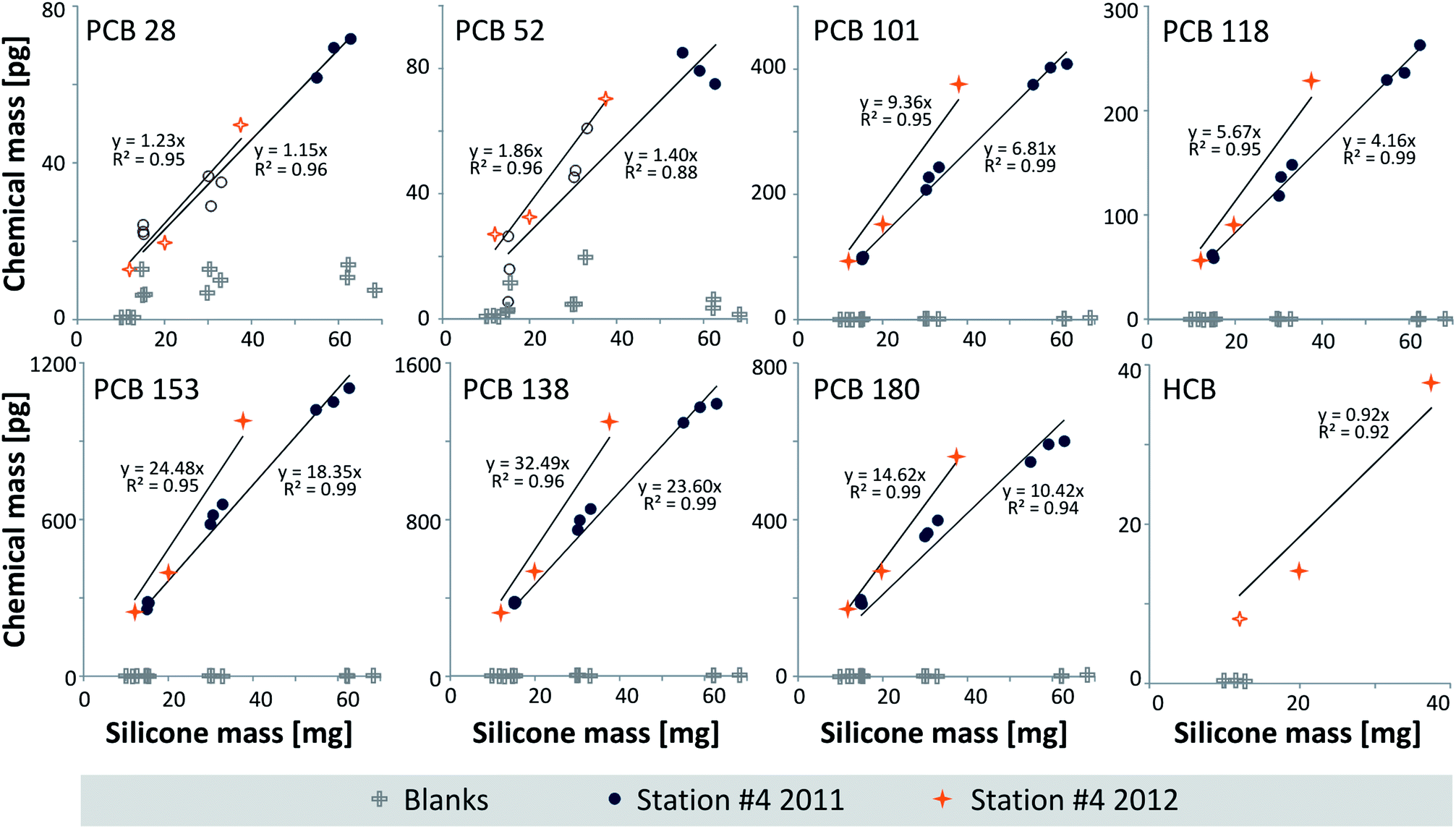Fig. 2 Mass [pg] of the chemical vs. silicone mass [mg] of the glass jar coatings equilibrated with Lake Ången sediment from station #4 sampled in 2011 and 2012. Blanks are also shown. Open symbols represent data <MQL (Table S3†). The HCB data from 2011 were <MQL. The PCB graphs indicate reproducible and artifact-free equilibrium sampling,²² whereas additional assessments (see the text and Fig. S1†) indicated underequilibration of PCBs 138 and 180 in the thickest coating of the 2011 data and PCB 180 at station #5. The p values of the linear regression through the origin for the 2011 dataset (n = 9) were <0.0001, whereas they were <0.008 for the 2012 dataset (n = 3, except for HCB, p = 0.011); data <MQL were included in this assessment.

In the sample extracts from sites #1 to #5 collected in 2012, HCB was mostly, and PCBs 28 and 52 were occasionally <MQL in the 1 μm silicone coatings and/or at site #4 that showed the lowest levels. There was good agreement between the 2011 and 2012 PCB data collected at station #4 (Fig. 2, with slopes not being significantly different), underlining the reproducibility of sampling and analytical methods and demonstrating low inter-annual variability in Lake Ången sediments. The concentrations at the five stations differed by up to a factor of 2.6 (PCB 101 between stations #3 and #4), with station #4 (2011) at the lower end (Fig. S1†).

3.4. Validation of the equilibrium sampling

As a validation measure,²⁹ the equilibrium partitioning concentrations in eel lipids (C_{Lip, eq}, eqn (2), Table S4 in the ESI†) were compared to the lipid-normalized concentrations in the eels (C_{Eel, Lip}, see below and Table S5 in the ESI†). The calculated C_{Lip, eq} were in good agreement with C_{Eel, lip}: in general, C_{Lip, eq} was between 21% (PCB 118) and 43% (PCB 101) lower than C_{Eel, Lip}; PCB 28, based on few data, was 62% lower.

The different silicone coating thicknesses on the glass jars²² resulted in linear plots of chemical mass versus silicone mass (Fig. 2) forced through the origin with R²s of 0.94–0.99 for the PCBs with 5–7 chlorines. For the remaining chemicals that were in part <MQL, R²s were 0.88–0.96. This is consistent with the sampler and the medium having achieved equilibrium, and at the same time showing no sign of sampling artifacts.²² Additional validation plots are given in Fig. S1† with the regression lines not forced through the origin. The intercepts were in most cases not statistically different from zero (ANOVA, Fig. S1†), which is consistent with equilibrium partitioning between the sediment and the silicone coatings having been reached. The only exceptions were PCBs 138 and 180 in the 2011 data from station #4 and PCB 180 in the sediment from station #5, which indicate slight under-equilibration or sample depletion in the jar with the thickest silicone coating. Eliminating the 8 μm thick coating from the 2011 data yields intercepts that are not statistically different from zero for PCBs 138 and 180.

As an additional validation measure for the coated glass jar data, we calculated the freely dissolved concentration in the interstitial pore water (C_{Sed, free}) of the sediment from station #4 from the silicone-coated glass jars (Table S6 in the ESI†) according to eqn (3). C_{Sed, free} are given both at 20 °C and extrapolated to the actual water temperature at the time of sediment sampling (6 °C) as described in ref. 14 and 19. Furthermore, C_{Sed, free} was calculated from the exhaustive extraction data (C_{Sed, OC} from station #4 (ref. 33)) according to eqn (4). The K_OC data used in this transformation were estimated as [0.35 × K_OW (ref. 25)] according to Seth et al.,³⁴ [0.63 × K_OW] according to Karickhoff et al.³⁵ and [0.98 × K_OW] according to Di Toro et al.,¹⁶ and the resulting C_{Sed, free} is included in Table S6.†C_{Sed, free} from the passive sampling approach was compared to C_{Sed, free} from the exhaustive extraction, showing reasonable agreement (Fig. S2 in the ESI†). The C_{Sed, free} dataset from passive sampling was by an average factor of 1.8 lower than the data obtained using the Seth et al.³⁴ relationship; it agreed well with the data from the Karickhoff et al.³⁵ relationship and exceeded the data from the Di Toro et al.¹⁶ relationship by an average factor of 1.5 (Fig. S2†). These differences in C_{Sed, free} derived from C_{Sed, OC} show that there is considerable uncertainty associated with the calculated C_{Sed, free} depending on the generic K_OC–K_OW relationship since the sorptive capacity of the OC is highly variable.^16,34,35

3.5. Exhaustive extraction of eels and sediments

The recoveries of the IS spiked before exhaustive extraction of eels by ultrasonication and sediments by Soxhlet extraction were comparable; they ranged from 28 to 112% (on average 80%) for the eels and from 61 to 115% (on average 84%) for the sediments. C_{Eel, Lip} of all analytes in the five eels are given in Table S5 in the ESI.† Due to high MQLs, HCB could not be quantified. PCB 28 was detected in all cases, but only quantified occasionally above the MQL. PCB 52 was <1.38 ng g⁻¹ lipid in the extracts of eel E. The concentrations of the PCBs with 5–7 chlorines were lower by a factor of 2.0 (PCBs 153 and 180) to 6.7 (PCB 101) (average 3.2) in eel E than in the eels with the highest concentrations. The C_{Sed, OC} of HCB could only be determined qualitatively, and PCBs 28 and 52 were <MQL. For the PCBs with 5 to 7 chlorines, C_{Sed, OC} ranged from 2.19 ± 0.21 (PCB 118) to 8.82 ± 0.79 (PCB 138) ng g⁻¹ OC.³³

3.6. Biota–sediment accumulation factors

We calculated BSAFs for HCB and the ‘indicator’ PCBs from the exhaustive extraction results for eels and sediments according to

BSAF = C_{Eel, Lip}/C_{Sed, OC} (5)

The obtained BSAFs are plotted in Fig. 3A. In this assessment, only semi-quantitative BSAFs were obtained for HCB, PCB 28 and PCB 52 since they were in part <MQL. For the PCBs with 5 to 7 chlorines, BSAFs ranged from 2.7 (PCB 101) to 12.7 (PCB 153).

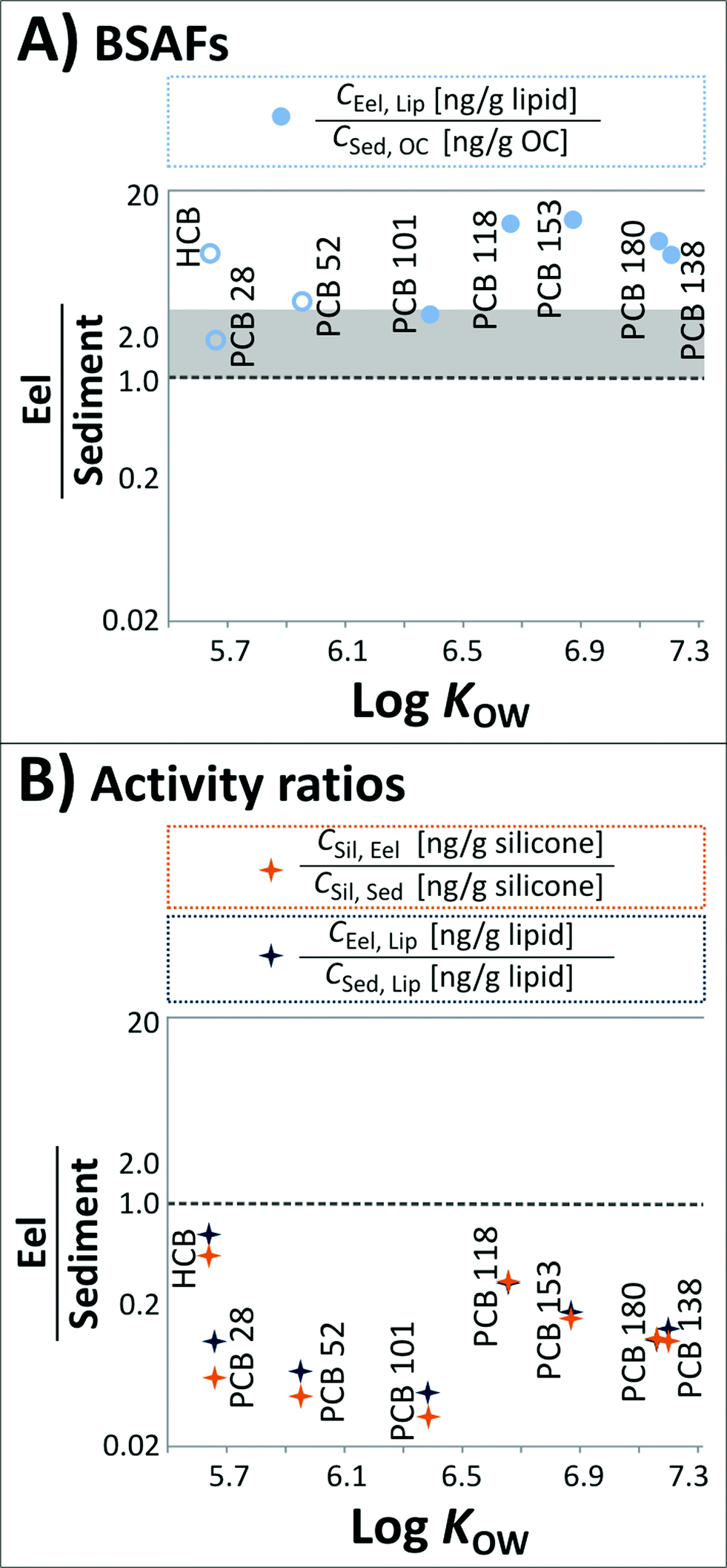Fig. 3 (A) BSAFs of HCB and the ‘indicator’ PCBs. Open symbols represent data that were in part <MQL. The data above the shaded area corresponding to BSAFs of 1–3 (depending on the supposed generic K_OC–K_OW relationship^16,34,35) indicate an enrichment of the chemicals in eels compared to sediments. (B) (i) Activity ratios [C_{Sil, Eel}/C_{Sil, Sed}] of HCB and the ‘indicator’ PCBs; (ii) ratios of C_{Eel, Lip} and their concentrations in model lipids at thermodynamic equilibrium with the sediments [C_{Sed, Lip} = C_{Sil, Sed} × K_Lip/Sil (ref. 24)] calculated from the silicone coatings of glass jars equilibrated with Lake Ången sediments. Averages of all quantifiable data are included.

4. Discussion

4.1. Observed levels of PCBs and HCB

The PCB concentrations in the five eels from Lake Ången are within the range reported for eels in Swedish lakes and coastal waters by the Swedish National Food Administration.^36,37 They are also within the range of PCB concentrations reported for Baltic Sea herring within the Swedish national environmental monitoring program.³⁸

We compared the Lake Ången sediment data with our earlier Baltic Sea sediment results from the Stockholm Archipelago.¹⁹ The average PCB concentrations in the silicone equilibrated with Lake Ången sediments are between a factor of 0.65 (PCB 52) and 2.36 (PCB 180), and on average 1.21, of the Stockholm Archipelago average. This good agreement of C_Sil equilibrated with sediments from Lake Ången and the Baltic Sea is consistent with the absence of point sources of PCBs and HCB to Lake Ången.

4.2. Thermodynamics of bioaccumulation

Different silicone polymers were used as the thin-film samplers (SSP-M823) for eels and the coated glass jar samplers (DC1-2577) for sediments. Therefore, K_DC/SSP (ref. 27) was applied for correction to directly compare the concentrations in the silicone polymers at equilibrium with the eels and the sediments. The ratios of chemical activities in eels (a_Eel) and sediments (a_Sed) were calculated according to

a_Eel/a_Sed = C_{Sil, Eel}/(C_{Sil, Sed}/K_DC/SSP) (6)

The activity ratio a_Eel/a_Sed for all compounds is below 1.0 (Fig. 3B) indicating a lower chemical activity in eels relative to sediments. Activities in silicone equilibrated with eel tissue are lower by a factor of 2.3 for HCB and factors of 3.5 (PCB 118) up to 31.1 (PCB 101) for PCBs.

We additionally calculated chemical concentrations in model lipids at thermodynamic equilibrium with the sediment (C_{Sed, Lip}) according to a modified version of eqn (1) that takes into account the differences in sorptive capacities of the applied silicone polymers:

C_{Sed, Lip} = (C_{Sil, Sed}/K_DC/SSP)K_Lip/Sil (7)

The obtained C_{Sed, Lip} was then compared to C_{Eel, Lip} from exhaustive extraction (Fig. 3B). The lipid-normalized concentrations in the eels were considerably lower than the equilibrium partitioning extrapolation from sediment to lipid, and the concentration ratios [C_{Eel, Lip}/C_{Sed, Lip}] were in good agreement with the concentration ratios on a silicone basis [C_{Sil, Eel}/C_{Sil, Sed}] (Fig. 3B). HCB is closest to equilibrium, whereas PCB 101 shows the largest disequilibrium between sediments and eels, followed by PCB 52, possibly due to biotransformation. Biotransformation of PCBs has been shown to be structure-dependent in fish, being greater for PCBs possessing vicinal hydrogen atoms in the meta/para positions such as PCBs 101 and 52.³⁹

4.3. Apparent disagreement between classical BSAFs and eel/sediment activity ratios

There is an apparent, perhaps surprising, discrepancy in the reported data between (i) ‘classical’ BSAFs being >1 (Fig. 3A) and (ii) ratios of chemical activities in eels and sediments being <1 (Fig. 3B). However, this disagreement can be explained by the higher sorptive capacities of biota lipids compared to sediment OC, which we assessed as described in Text S2 in the ESI.† The differences in sorptive capacities imply that a BSAF of 1–3 (depending on the assumed K_OC–K_OW relationship, (ref. 16, 34 and 35)) should not be used as a reference for equilibrium partitioning between biota lipids and sediment OC. Rather, equilibrium partitioning is indicated by BSAFs in the range of the lipid/OC partition ratios (K_Lip/OC).

Since the sorptive capacities of biota lipids have been shown not to differ substantially between a large range of different lipids (i.e., olive oil, fish oil and seal oil²⁴ and linseed oil, soybean oil, olive oil, fish oil, milk fat and goose fat⁴⁰), the variable characteristics of the sediment organic carbon between ecosystems are likely to be decisive for differences of K_Lip/OC. Correspondingly, K_Lip/OC are sediment-specific, and our calculated K_Lip/OC for Lake Ången sediments were 29.3 (PCB 118), 31.2 (PCB 101), 36.1 (PCB 138), 48.3 (PCB 153) and 49.7 (PCB 180).

The observed BSAFs were lower than K_Lip/OC, which also indicates under-equilibration of biota lipids with sediment OC in agreement with the obtained activity ratios of <1 (Fig. 3B). The Lake Ången dataset hence suggests that differences in the sorptive capacities of lipids and OC may be considerable and deserve evaluation. The differences can be assessed for other systems using the proposed passive sampling approach.

4.4. Factors influencing the eel/sediment activity ratios

As discussed above, concentration ratios on both a silicone basis [C_{Sil, Eel}/C_{Sil, Sed}] and a lipid basis [C_{Eel, Lip}/C_{Sed, Lip}] suggest an under-equilibration of the eels relative to the sediments (Fig. 3B). Considering K_Lip/OC for Lake Ången sediments, BSAFs give the same indication. We can formulate a range of hypotheses to explain this finding.

The first is that a process or group of processes may increase the chemical activity in the sediments compared to the overlying water. Higher activities in sediments can, for instance, occur as the result of falling levels in the environment to which a slower response by the sediment compartment compared to water and air can be expected.^41,42 Higher chemical activities in sediments relative to water can also be driven by ongoing sediment OC diagenesis that can reduce the sorptive capacity of the sediments and thereby increase the chemical activity of persistent chemicals in the sediments.⁴³ While both these processes are expected to occur in Lake Ången, they will only induce significant sediment–water disequilibrium if the transfer of chemicals from sediments to the water column is slow compared to the loss of chemicals from the water column to the air, which seems unlikely for this shallow lake with an average depth of 5 m.

The second hypothesis is that reduced activity in the water column results from primary production and subsequent sorption of persistent chemicals to phytoplankton. Nizzetto et al.⁴⁴ reported that this process can act as an efficient biological pump, dramatically decreasing freely dissolved concentrations in the water column. For food webs for which contaminant exposure is primarily determined by the water column, this situation could result in an exposure below that expected from the sediments. While this process is very efficient under stratified conditions and during the peaks of primary production,⁴⁴ it seems unlikely that the overall annual effect alone is sufficient to explain the considerably lower chemical activities in the eels compared to sediments. Furthermore, this effect should be of minor importance in a shallow lake such as Lake Ången where stratification will seldom occur. The observation of HCB being closer to equilibrium than the more hydrophobic PCBs is consistent with this second explanation, since phytoplankton-related contaminant depletion in the water column is of higher importance with increasing hydrophobicity.⁴⁵

A third hypothesis is that the sediment samples were not representative of the actual habitat of the eels. However, the small range in C_{Sil, Eel} and in C_{Sil, Sed} (a factor of 2.6 and 3.1, respectively, for PCB 153, n = 14 and 24, respectively) compared to the extent of the thermodynamic gradient (C_{Sil, Eel}/C_{Sil, Sed} = 0.16) speaks against this explanation. Furthermore, the eels had very likely been present in the lake for more than 20 years and therefore had ample opportunity to migrate throughout the lake.

The fourth hypothesis is that enhanced biotransformation could contribute to lower chemical activities in the eels. However, we do not believe that this process could be sufficiently fast to be the dominant factor determining our measured activity ratios.

Finally, it is possible to hypothesize that there is an error in the passive sampling methodology. We have carefully evaluated the methods with respect to equilibration and a range of potential artifacts^22,29 as described above. A lack of equilibration during sediment sampling is unlikely for the vast majority of the presented data (see above), and even if it was the case, it could not explain the observed activity ratios, since under-equilibration would imply an even larger disequilibrium between eels and sediments. A change of sorptive properties of the silicone when immersed in sediments and biota can be ruled out based on a previous study.²⁰ A lack of equilibration during in-tissue sampling would bias the ratios in the observed direction, but is unlikely based on previous time series studies,^21,32 experiments using different silicone thicknesses²¹ and due to the inclusion of a safety factor of approx. 6 times prolonged sampling times. Furthermore, this effect would also become obvious when comparing C_{Lip, eq} (Table S4†) with C_{Eel, Lip} (Table S5†). Finally, the observation of HCB being closer to equilibrium than the more hydrophobic PCBs is an additional indication of well-calibrated methods, since HCB in general is a faster-equilibrating compound which leads to smaller activity gradients than those observed for PCBs.

In summary, it is at present difficult to identify a single hypothesis or mechanism that can explain the observed disequilibrium between eels and sediments. The activity ratios <1 might rather be the result of several processes, some of them being discussed above. This study illustrates that the ‘chemometer’ approach can effectively indicate thermodynamic differences in real environmental systems, whereas additional studies may be required to fully explain the causes of these differences. The ‘chemometer’ measurements might thus inspire research on phenomena and processes that are not yet sufficiently understood to be integrated into environmental fate models.

5. Conclusions

This study describes the parallel application of passive equilibrium samplers as ‘chemometers’ in eels and sediments from the same ecosystem. The ‘chemometer’ approach provided novel, thermodynamically based insight into bioaccumulation in Lake Ången and is highly promising for studying thermodynamic controls on persistent organic contaminants in a variety of systems.

Acknowledgements

The authors gratefully acknowledge Mona Blomqvist, Sven-Erik Blomqvist, Sören Lehmann and Johan Löwen for allowing us to carry out sampling on their property and Sören Lehmann for providing us with eel samples. We acknowledge Urs Berger, Andreas Hägerroth, Per-Åke Hägerroth, Daniel Johansson and Damien Bolinius for their assistance during sampling, and Margit Møller Fernqvist for the coating of the glass jars. We thank Ulla Eriksson and Jörgen Ek for their assistance in the laboratory, Cecilia Bandh and Yngve Zebühr for the GC/HRMS analyses and Heike Siegmund for the TOC analyses. We thank the anonymous reviewers for their comments, which helped us to improve the manuscript. This research was funded by The Long-range Research Initiative of The European Chemical Industry Council (CEFIC, LRI-ECO14-15.2), the Swedish Research Council VR (2011-3890) and the EU Commission (OSIRIS, GOCE-037017; Marie Curie Intra European Fellowship, PIEF-GA-2008-219675).

References

1. J. A. Arnot and F. A. P. C. Gobas, Environ. Rev., 2006, 14, 257–297.
2. K. E. Clark, F. A. P. C. Gobas and D. Mackay, Environ. Sci. Technol., 1990, 24, 1203–1213.
3. F. A. P. C. Gobas, X. Zhang and R. Wells, Environ. Sci. Technol., 1993, 27, 2855–2863.
4. L. P. Burkhard, J. A. Arnot, M. R. Embry, K. J. Farley, R. A. Hoke, M. Kitano, H. A. Leslie, G. R. Lotufo, T. F. Parkerton, K. G. Sappington, G. T. Tomy and K. B. Woodburn, Integr. Environ. Assess. Manage., 2012, 8, 17–31.
5. F. A. P. C. Gobas, W. de Wolf, L. P. Burkhard, E. Verbruggen and K. Plotzke, Integr. Environ. Assess. Manage., 2009, 5, 624–637.
6. A. M. H. deBruyn and F. A. P. C. Gobas, Environ. Toxicol. Chem., 2007, 26, 1803–1808.
7. S. Endo, J. Bauerfeind and K.-U. Goss, Environ. Sci. Technol., 2012, 46, 12697–12703.
8. S. Endo, T. N. Brown and K.-U. Goss, Environ. Sci. Technol., 2013, 47, 6630–6639.
9. G. Cornelissen, Ö. Gustafsson, T. D. Bucheli, M. T. O. Jonker, A. A. Koelmans and P. C. M. van Noort, Environ. Sci. Technol., 2005, 39, 6881–6895.
10. D. Mackay, Environ. Sci. Technol., 1979, 13, 1218–1223.
11. T. Clark, K. Clark, S. Paterson, D. Mackay and R. J. Norstrom, Environ. Sci. Technol., 1988, 22, 120–127.
12. P. Mayer, J. Tolls, J. L. M. Hermens and D. Mackay, Environ. Sci. Technol., 2003, 37, 184A–191A.
13. E. Webster, D. Mackay and K. Qiang, J. Great Lakes Res., 1999, 25, 318–329.
14. R. P. Schwarzenbach, P. M. Gschwend and D. M. Imboden, Environmental Organic Chemistry. John Wiley, New York, NY, USA, 1993.
15. F. Reichenberg and P. Mayer, Environ. Toxicol. Chem., 2006, 25, 1239–1245.
16. D. M. Di Toro, C. S. Zarba, D. J. Hansen, W. J. Berry, R. C. Swartz, C. E. Cowan, S. P. Pavlou, H. E. Allen, N. A. Thomas and P. R. Paquin, Environ. Toxicol. Chem., 1991, 10, 1541–1583.
17. D. Mackay, J. Arnot and R. E. Bailey, Integr. Environ. Assess. Manage., 2010, 7, 248–255.
18. P. Mayer, T. F. Parkerton, R. G. Adams, J. C. Cargill, J. Gan, T. Gouin, P. M. Gschwend, S. B. Hawthorne, P. Helm, G. Witt, J. You and B. I. Escher, Integr. Environ. Assess. Manage., 2014 DOI:10.1002/ieam.1508 (in press).
19. A. Jahnke, P. Mayer and M. S. McLachlan, Environ. Sci. Technol., 2012, 46, 10114–10122.
20. A. Jahnke and P. Mayer, J. Chromatogr., A, 2010, 1217, 4765–4770.
21. A. Jahnke, P. Mayer, D. Broman and M. S. McLachlan, Chemosphere, 2009, 77, 764–770.
22. F. Reichenberg, F. Smedes, J. Å. Jönsson and P. Mayer, Chem. Cent. J., 2008, 2, 8.
23. K. Mäenpää, M. T. Leppänen, F. Reichenberg, K. Figueiredo and P. Mayer, Environ. Sci. Technol., 2011, 45, 1041–1047.
24. A. Jahnke, M. S. McLachlan and P. Mayer, Chemosphere, 2008, 73, 1575–1581.
25. U. Schenker, M. MacLeod, M. Scheringer and K. Hungerbühler, Environ. Sci. Technol., 2005, 39, 8434–8441.
26. L. Shen and F. Wania, J. Chem. Eng. Data, 2005, 50, 742–768.
27. D. Gilbert, G. Witt, F. Smedes and P. Mayer, Intercalibrating passive sampling and dosing polymers based on polymer–polymer partition ratios of PCBs, PAHs and organochlorine pesticides, manuscript in preparation.
28. S. Jensen, L. Reutergårdh and B. Jansson, FAO Fish. Tech. Pap., 1983, 212, 21–33.
29. A. Jahnke, P. Mayer, M. Adolfsson-Erici and M. S. McLachlan, Environ. Toxicol. Chem., 2011, 30, 1515–1521.
30. C. Bandh, E. Björklund, L. Mathiasson, C. Näf and Y. Zebühr, Environ. Sci. Technol., 2000, 34, 4995–5000.
31. F. Smedes, R. W. Geertsma, T. van der Zande and K. Booij, Environ. Sci. Technol., 2009, 43, 7047–7054.
32. L. Ossiander, F. Reichenberg, M. S. McLachlan and P. Mayer, Chemosphere, 2008, 71, 1502–1510.
33. A. Jahnke, P. Mayer, M. S. McLachlan, H. Wickström and M. MacLeod, Oral presentation Thermodynamic bioaccumulation study using PDMS-based passive equilibrium sampling in a Swedish lake at the SETAC Europe 22nd annual meeting, Glasgow, Scotland, 16 May 2013.
34. R. Seth, D. Mackay and J. Muncke, Environ. Sci. Technol., 1999, 33, 2390–2394.
35. S. W. Karickhoff, D. S. Brown and T. A. Scott, Water Res., 1978, 13, 241–248.
36. Report 9/2007, Risk assessment of persistent chlorinated and brominated environmental pollutants in food, http://www.slv.se/sv/grupp3/Rapporter/Kemiska-amnen/, accessed December 31, 2013.
37. Report 21/2012 Dioxin and PCB concentrations in fish and other foodstuff 2000–2011 (in Swedish), http://www.slv.se/sv/grupp3/Rapporter/Kemiska-amnen/, accessed December 31, 2013.
38. Swedish monitoring data at http://www3.ivl.se/db/plsql/dvsb_pcb$.startup (in Swedish), accessed December 31, 2013.
39. A. H. Buckman, C. S. Wong, E. A. Chow, S. B. Brown, K. R. Solomon and A. T. Fisk, Aquat. Toxicol., 2006, 78, 176–185.
40. A. Geisler, S. Endo and K.-U. Goss, Environ. Sci. Technol., 2012, 46, 9519–9524.
41. L. P. Burkhard, P. M. Cook and M. T. Lukasewycz, Environ. Sci. Technol., 2004, 38, 5297–5305.
42. L. P. Burkhard, P. M. Cook and M. T. Lukasewycz, Environ. Sci. Technol., 2008, 42, 3615–3621.
43. F. A. P. C. Gobas and L. G. MacLean, Environ. Sci. Technol., 2003, 37, 735–741.
44. L. Nizzetto, R. Gioia, J. Li, K. Borgå, F. Pomati, R. Bettinetti, J. Dachs and K. C. Jones, Environ. Sci. Technol., 2012, 46, 3204–3211.
45. J. Dachs, S. J. Eisenreich, J. E. Baker, F. C. Ko and J. D. Jeremiason, Environ. Sci. Technol., 1999, 33, 3653–3660.

---

Footnote

† Electronic supplementary information (ESI) available. See DOI: 10.1039/c3em00589e

---