 Open Access Article
 This Open Access Article is licensed under a
 Creative Commons Attribution 3.0 Unported Licence
The 6Hankel asymptotic approximation for the uniform description of rainbows and glories in the angular scattering of state-to-state chemical reactions: derivation, properties and applications
Chengkui
Xiahou
and
J. N. L.
Connor
*
School of Chemistry, The University of Manchester, Manchester M13 9PL, England, UK. E-mail: j.n.l.connor@manchester.ac.uk
First published on 31st January 2014
Abstract
This paper considers the asymptotic (semiclassical) analysis of a forward glory and a rainbow in the differential cross section (DCS) of a state-to-state chemical reaction, whose scattering amplitude is given by a Legendre partial wave series (PWS). A recent paper by C. Xiahou, J. N. L. Connor and D. H. Zhang [Phys. Chem. Chem. Phys., 2011, 13, 12981] stated without proof a new asymptotic formula for the scattering amplitude, which is uniform for a glory and a rainbow in the DCS. The new formula was designated “6Hankel” because it involves six Hankel functions. This paper makes three contributions: (1) we provide a detailed derivation of the 6Hankel approximation. This is done by first generalizing a method described by G. F. Carrier [J. Fluid Mech., 1966, 24, 641] for the uniform asymptotic evaluation of an oscillating integral with two real coalescing stationary phase points, which results in the “2Hankel” approximation (it contains two Hankel functions). Application of the 2Hankel approximation to the PWS results in the 6Hankel approximation for the scattering amplitude. We also test the accuracy of the 2Hankel approximation when it is used to evaluate three oscillating integrals of the cuspoid type. (2) We investigate the properties of the 6Hankel approximation. In particular, it is shown that for angles close to the forward direction, the 6Hankel approximation reduces to the “semiclassical transitional approximation” for glory scattering derived earlier. For scattering close to the rainbow angle, the 6Hankel approximation reduces to the “transitional Airy approximation”, also derived earlier. (3) Using a J-shifted Eckart parameterization for the scattering matrix, we investigate the accuracy of the 6Hankel approximation for a DCS. We also compare with angular scattering results from the “uniform Bessel”, “uniform Airy” and other semiclassical approximations.
I. Introduction
The angular scattering of a state-to-state chemical reaction contains fundamental information on the dynamics and mechanism of the reaction.1 However, it has often proven difficult to quantitatively understand the physical content contained within a plot of the differential cross section (DCS) versus reactive scattering angle. Consider, for example, the F + H2 → FH + H reaction, whose angular scattering was measured in the famous crossed molecular-beam experiments of Neumark et al.2 in 1985. It took 19 years before the enhanced forward peak in the small-angle scattering of the product FH(vf = 3) vibrational state was identified3 as a glory. And it took 24 years before the scattering at larger angles in the DCS was recognized4 as a rainbow.More recently (in 2008), state-of-the-art DCS measurements for the F + H2 reaction were reported by Wang et al.5 using quantum-state-selected crossed molecular beams. An analysis of the angular scattering by ourselves and Zhang6 again revealed the presence of glories and rainbows in the FH(vf = 3) DCSs; they are also accompanied by diffraction oscillations arising from nearside–farside interference.
The analyses in ref. 3, 4 and 6 used powerful asymptotic (semiclassical) techniques to extract physical information from the large number of interfering partial waves which contribute to the scattering amplitude. Two different asymptotic theories were employed: One theory3,7 led to the uniform glory approximation (and subsidiary approximations), whilst the second theory8 resulted in the uniform (and transitional) rainbow approximations. A disadvantage of these theoretical treatments is that the uniform glory approximation becomes non-uniform for rainbow scattering, and vice versa. By a uniform approximation, we mean one in which the error remains approximately constant as a parameter, such as the reactive scattering angle, passes through certain critical values, such as zero (for a forward glory) or the rainbow angle.3,4,6–8 A transitional approximation is one in which the error remains small in the neighbourhood of these critical values, but the error usually increases as the parameter moves away from the critical values.3,4,6–8
It is desirable to develop new asymptotic scattering theories that are uniform for both forward glory and rainbow scattering. This was partially done in our paper with Zhang,6 where we stated without proof a new asymptotic approximation for the scattering amplitude that is valid for both a glory and a rainbow. We called our new result, the 6Hankel asymptotic approximation, since it contains six Hankel functions.6 For the DCS, our new result is a generalization to reactive scattering of a formula given by Miller9 for elastic scattering.
The purpose of this paper is: (1) to present a derivation of the 6Hankel approximation, (2) to discuss its properties, and (3) to assess its accuracy for the DCS of a chemical reaction. In our DCS computations, we use a J-shifted Eckart parameterization of the scattering (S) matrix,10,11 as it allows flexibility in the location of the rainbow angle, thereby allowing us to test the 6Hankel approximation over a wide angular range.
For information on the mathematical description of glories and rainbows, we refer to the extensive review by Adam.12 Earlier work on the role of forward glories in the DCSs of chemical reactions can be found in ref. 3, 6, 7, 10, 11 and 13–17. Likewise the role of rainbows is discussed in ref. 4 and 6.
In order to describe a rainbow, we first must consider the uniform asymptotic evaluation of a one-dimensional oscillating integral with two coalescing stationary phase points. This is done in Section II. In particular, we generalize a method described by Carrier.18 He assumes that the phase of the integrand is an odd function of x and that the pre-exponential factor is an even function of x, where x is the integration variable. We extend his result to the case when neither of these symmetry properties holds. We call our generalization, the 2Hankel asymptotic approximation, since it involves two Hankel functions. We also investigate the limit when the stationary phase points coalesce, which leads to the transitional Airy approximation4,6,8 for rainbow scattering.
Section III applies the 2Hankel approximation to the scattering amplitude for a chemical reaction, when it is given by a Legendre partial wave series, thereby providing a derivation of the 6Hankel approximation. The limit when the scattering angle tends to zero is investigated, resulting in the semiclassical transitional approximation3 previously derived for glory scattering.
The J-shifted Eckart parameterization for the S matrix10,11 is defined in Section IV. The values of the parameters are chosen so that the rainbow angle occurs at a large value, namely 109.2° in the centre-of-mass reference frame. This allows us to conduct a better test of the accuracy of the 6Hankel approximation than previously, which used numerical S matrix data.6 An important point is that the 6Hankel formula is generic, i.e., it also applies to numerous chemical reactions at numerous different energies which have S matrix properties analogous to the J-shifted Eckart parameterization.
Section V describes our results for the DCS using the 6Hankel and other semiclassical approximations. In order to provide additional physical insight into interference structure in the DCS, we have also applied nearside–farside (NF) theory19,20 and local angular momentum (LAM) theory,21–24 in both cases including up to three resummations of the partial wave series.21–24 We also make contact with complex angular momentum (or Regge pole) theory, which has been used to calculate DCSs.25–27
Our Conclusions are in Section VI. The Appendix describes a test of the 2Hankel approximation when it is applied to three oscillating integrals of the cuspoid type.28,29
Finally, we emphasize that there is a long tradition in the chemical physics literature of papers concerned with the asymptotic evaluation of oscillating integrals, see for example ref. 3, 4, 6–17, 20, 23, 25–28 and 30–36.
II. Uniform asymptotic integration: the 2Hankel approximation
IIA. Introduction
This section is concerned with the uniform asymptotic evaluation of the oscillating integral: | (1) |
The convenient notations xi = xi(α), gi = g(xi), fi = f(α;xi), fi′ = f′(α;x)|x=xi, fi′′ = f′′(α;x)|x=xi and fi′′′ = f′′′(α;x)|x=xi for i = 0, 1, 2 will often be employed in the following. In our application in Section III, f(α;x) has a linear dependence on α of the type, ±αx, which means that the second and third derivatives of f(α;x) are independent of α. But note that fi′′ and fi′′′ do depend on α via the xi = xi(α).
Given the above assumptions, two cases arise, depending on whether f(α;x) → +∞ or → −∞ as x → +∞ [or equivalently, f(α;x) → −∞ or → +∞ as x → −∞]. These two cases are illustrated in Fig. 1, where f(α;x) is given by simple polynomial functions. The black solid curves for f(α;x) in Fig. 1 possess a local maximum and a local minimum. Also illustrated are the curves (blue solid) when the two stationary points have coalesced for α = α0. The two cases have the following properties, which we use later:
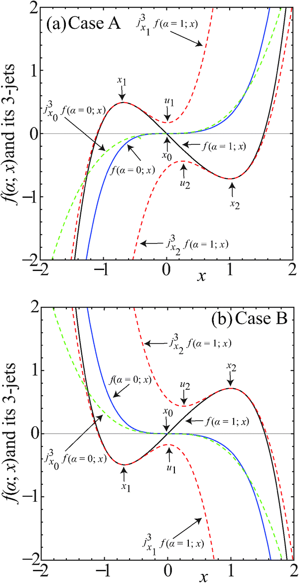 | ||
| Fig. 1 Properties of the phase f(α;x) and three of its 3-jets. (a) Case A. Black solid line: f(α;x) = −αx + x3/3 − x4/4 + x5/5 for α = 1. Its stationary phase points are given by, x1 ≈ −0.682328 (local maximum) and x2 = 1 (local minimum). Lower red dashed curve: The 3-jet at x2, jx23f(α = 1;x). Its stationary phase points are denoted, u2 = 1/4 (local maximum) and x2 = 1 (local minimum). Upper red dashed curve: The 3-jet at x1, jx13f(α = 1;x). Its stationary phase points are denoted, x1 ≈ −0.682328 (local maximum) and u1 ≈ 0.00804454 (local minimum). Blue solid curve: f(α = 0;x) = x3/3 − x4/4 + x5/5. Its two stationary phase points have coalesced at x0 = 0. Green dashed curve: The 3-jet at x0, jx03f(α = 0;x) = x3/3. Its two stationary phase points have coalesced at x0 = 0. (b) Case B. Black solid line: f(α;x) = −(−αx + x3/3 − x4/4 + x5/5) for α = 1. Its stationary phase points are given by, x1 ≈ −0.682328 (local minimum) and x2 = 1 (local maximum). Upper red dashed curve: The 3-jet at x2, jx23f(α = 1;x). Its stationary phase points are denoted, u2 = 1/4 (local minimum) and x2 = 1 (local maximum). Lower red dashed curve: The 3-jet at x1, jx13f(α = 1;x). Its stationary phase points are denoted, x1 ≈ −0.682328 (local minimum) and u1 ≈ 0.00804454 (local maximum). Blue solid curve: f(α = 0;x) = −(x3/3 − x4/4 + x5/5). Its two stationary phase points have coalesced at x0 = 0. Green dashed curve: The 3-jet at x0, jx03f(α = 0;x) = −x3/3. Its two stationary phase points have coalesced at x0 = 0. | ||
Case A – see Fig. 1(a)
For x1 < x2 so that α ≠ α0
| f1 > f2, f1′ = f2′ = 0, |
| f1′′ < 0, f2′′ > 0, f1′′′ > 0, f2′′′ > 0 |
For x1 = x2 = x0 so that α = α0
| f0′ = 0, f0′′ = 0, f0′′′ > 0 |
Case B – see Fig. 1(b)
For x1 < x2 so that α ≠ α0
| f1 < f2, f1′ = f2′ = 0, |
| f1′′ > 0, f2′′ < 0, f1′′′ < 0, f2′′′ < 0 |
For x1 = x2 = x0 so that α = α0
| f0′ = 0, f0′′ = 0, f0′′′ < 0 |
Remarks:
• It is also assumed that g(x) does not possess any singularities or zeros near to the stationary phase points. A modified treatment can be given if this is not the case (e.g., see ref. 37 and 38, for example).
• If f(α;x) = −f(α; −x), i.e., f is an odd function of x, then x1 = −x2.
• If f(α;x) possesses more than two real stationary points, then the following derivation is valid locally in the region of the two coalescing stationary points,8,28 provided that the additional stationary points are well separated from the coalescing pair.
• The mathematical level of our derivations is similar to that of ref. 8 by one of us (JNLC) and Marcus (hereafter referred to as CM). The CM paper applied a different technique, that of Chester, Friedman and Ursell,39 for the uniform asymptotic evaluation of an oscillating integral with two coalescing saddle points. In particular, CM presented the Chester et al. technique in an accessible, yet general, way, making it straightforward to apply to problems in molecular scattering theory.
A comparison of Fig. 1(a) and (b), shows that Cases A and B are related by a minus sign. In the following, we focus only on Case A, since the uniform asymptotic theory for Case B is similar. We have chosen Case A because it is used in our analysis of a reactive DCS in Section III.
IIB. Two limiting cases
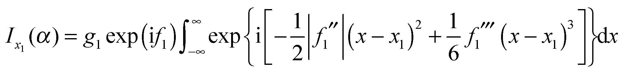
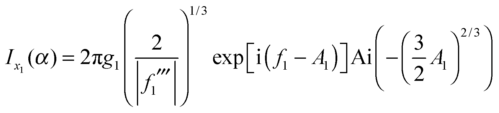
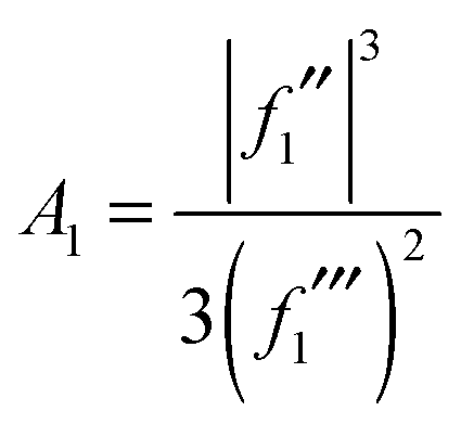
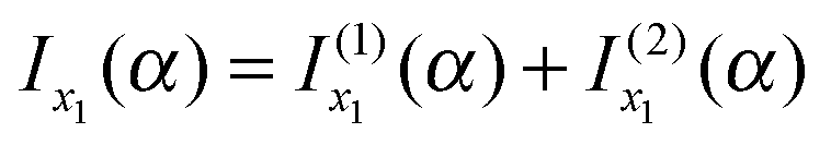
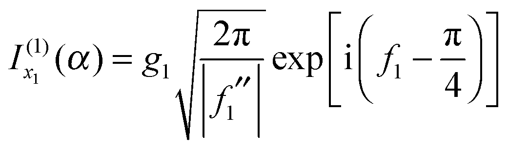
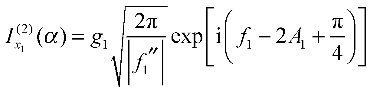
Before proceeding, it is helpful to write down results for I(α) in two limiting cases. The results we require can be found in CM. The first limiting case is when x1 and x2 are well separated. Then the simple stationary phase approximation (SPA) can be applied at both stationary points, which results in (from ref. 8) | (2) |
The second limiting case is when α ≈ α0 so that x1 ≈ x0 ≈ x2. We make a third-order Taylor series expansion of f(α;x) at the point x0
| f(α;x) ≈ f(α;x0) + f′(α;x0)(x − x0) + ⅙f′′′(α;x0)(x − x0)3 | (3) |
 | (4) |
 | (5) |
In the following, to avoid repeating phrases like “the kth-order Taylor series expansion of f(α;x) at the point xi”, we will often use the concept of a k-jet,40,41 which is defined as the Taylor series expansion of order k for f(α;x) at the point xi. For example, eqn (3) written as a 3-jet is
| jx03f(α;x) = f(α;x0) + f′(α;x0)(x − x0) + ⅙f′′′(α;x0)(x − x0)3 | (6) |
Note: all k-jets in this paper are functions and not members of a polynomial ring.
The problem now is to deduce a uniform approximation which reduces to eqn (2) and (4) in the appropriate limits.
IIC. Extension of Carrier's method
The basic idea of Carrier is to use 3-jets at the points x1 and x2, similar to eqn (3) or (6) for the point x0. This seems straightforward and physically reasonable, but Fig. 1(a) shows there is a serious problem. We see that the 3-jet at x2 is accurate close to x2, but it possesses another stationary point, say u2 = u2(α), which is quite different from x1. This implies that the approximation to I(α) using the 3-jet at x2, denoted Ix2(α), will be quite different from I(α), unless f(α;x) and jx23f(α;x) are very similar as functions of x. Evidently we must eliminate the contribution from the additional stationary point u2.
Similar remarks apply if the 3-jet at x1 is used – see Fig. 1(a); we must eliminate the contribution from the additional stationary point u1. And similarly for Case B in Fig. 1(b). Eliminating the unwanted contributions from u1 and u2 is the essence of our derivation.
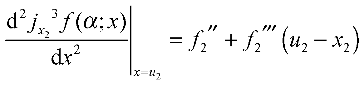
| jx23f(α;x) = f2 + ½f2′′(x − x2)2 + ⅙f2′′′(x − x2)3 | (7) |
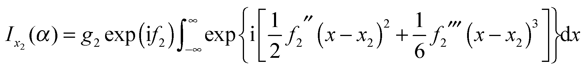 | (8) |
| x2 (by construction) | (9) |
| u2 = x2 − (2f2′′/f2′′′) | (10) |
Next we use the identity
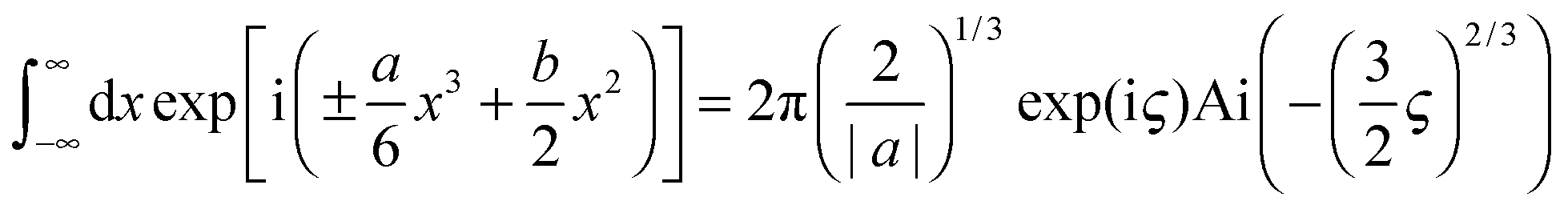 | (11) |
| ς = b3/(3a2) |
 | (12) |
 | (13) |
Next we use the following identity connecting Ai(•) and Hankel functions of the first and second kinds, H(1)1/3(•) and H(2)1/3(•) respectively, both of order one-third.42
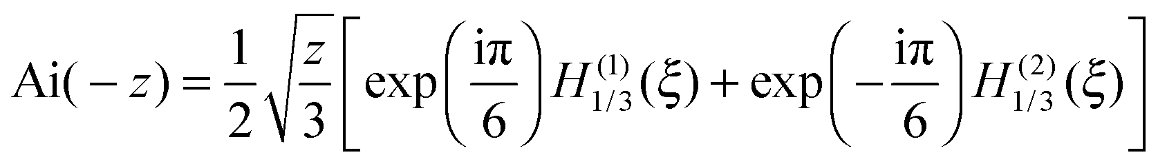 | (14) |
ξ = ⅔z3/2 or equivalently, z = (![[/]](https://www.rsc.org/images/entities/char_e0ee.gif) ξ)2/3 ξ)2/3 | (15) |
where
 | (16) |
 | (17) |
Next we consider the limit where x2 and u2 are well separated, so we can use the following asymptotic approximations for the Hankel functions43 as x → ∞
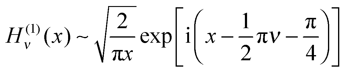 | (18) |
 | (19) |
 and
and  the results
 | (20) |
 | (21) |
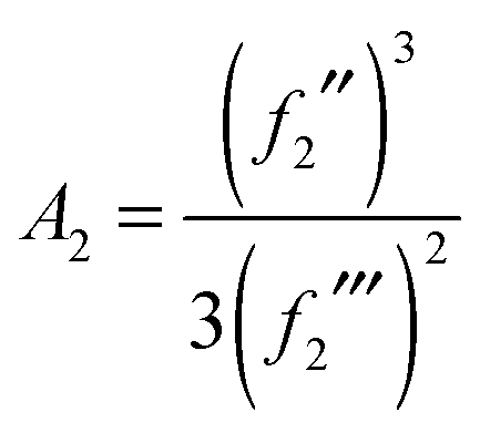
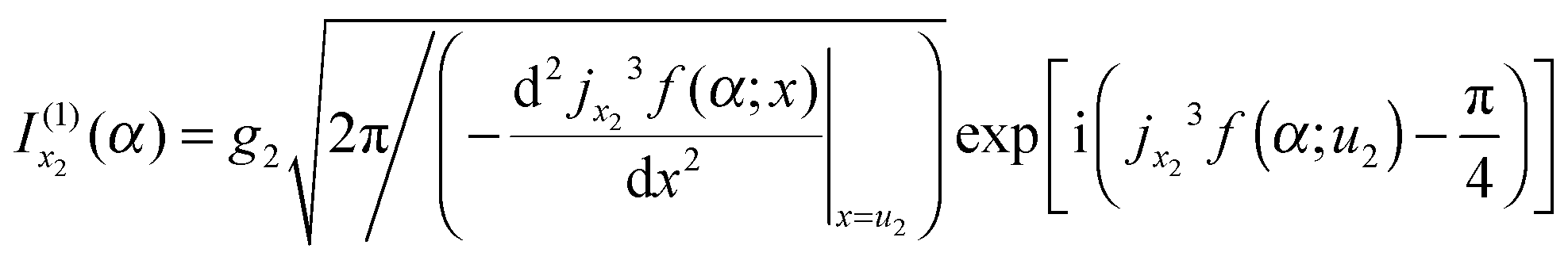
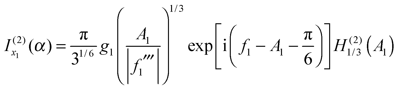
 is the simple stationary phase result for x2, as given by the second term on the rhs of eqn (2). This suggests the other integral,
  , is associated with the simple stationary phase result at u2. We now confirm this suggestion by expressing f2, A2 and f2′′ in eqn (20) in terms of u2 rather than x2.
From eqn (7), we have for x = u2
| jx23f(α;u2) = f2 + ½f2′′(u2 − x2)2 + ⅙f2′′′(u2 − x2)3 |
| jx23f(α;u2) = f2 + 2A2 | (22) |
and so for x = u2

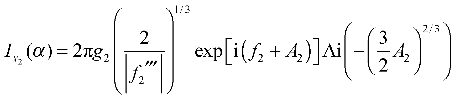
which simplifies to
 | (23) |
 | (24) |
 that we must eliminate from our theory, since eqn (24) may be quite different from the simple stationary phase result at x1 for I(α), as given by the first term on the rhs of eqn (2), namely
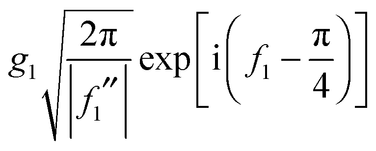
Note: The fact that f(α;x) has a maximum at x = x1 did not play an essential role in the argument that  should be retained and
  discarded when f(α;x) is approximated by jx23f(α;x). Thus if f(α;x) increases monotonically for x < x2, we would still retain
  and discard
  when using jx23f(α;x). Also, if in eqn (1), g(x) = constant, then trivially g(x2) = g(u2).
In the next section, we repeat the above analysis using the 3-jet at x1 rather than x2.
The 3-jet at x1 is given by
| jx13f(α;x) = f1 − ½|f1′′|(x − x1)2 + ⅙f1′′′(x − x1)3 | (25) |
 | (26) |
u 1 = x1 + (2|f1′′|/f1′′′) and x1 (by construction). Next we apply the identity (11) to eqn (26) obtaining
 | (27) |
 | (28) |
We again use the relations (14) and (15) connecting Ai(•) and the Hankel functions of the first and second kinds. This lets write eqn (27) as the sum of two terms
 | (29) |
 | (30) |
Next we consider the limit where x1 and u1 are sufficiently well separated that we can use the asymptotic approximations for the Hankel functions, as given by eqn (18) and (19) for x → ∞ with ν = 1/3. We obtain
 | (31) |
 | (32) |
 is the simple stationary phase result at x1, given by the first term on the rhs of eqn (2). Hence
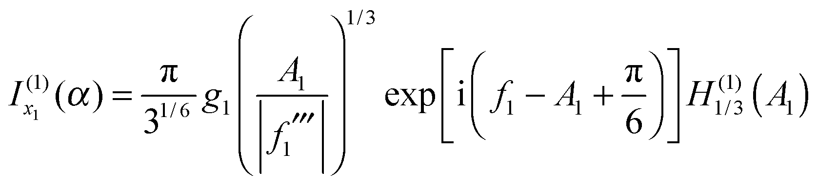
  should be associated with the simple stationary phase result at u1. We confirm this suggestion by manipulations in which f1, A1 and f1′′ in eqn (32) are expressed in terms of u1 rather than x1 –these manipulations are analogous to those in Section IIC.2 for eqn (20). It is found that
  can be written in the alternative form
 | (33) |
 that we must eliminate from our theory. Note that eqn (33) may be quite different from the simple stationary phase result at x2 for I(α), which is given by the second term on the rhs of eqn (2), namely
Note: The fact that f(α;x) has a minimum at x = x2 did not play an essential role in the argument that  should be retained and
  discarded when f(α;x) is approximated by jx13f(α;x). Thus if f(α;x) decreases monotonically for x > x1, we would still retain
  and discard
  when using jx13f(α;x). This observation is used in Section IIIC for the nearside scattering of the J-shifted Eckart parametrization of the S matrix. Also, if in eqn (1), g(x) = constant, then trivially g(x1) = g(u1).
 and
and  [i.e., eqn (29) and (17) respectively]. But we drop
  and
and  [i.e., eqn (30) and (16) respectively] because they correspond to unwanted contributions from the stationary phase points u1 and u2 respectively, which arise when f(α;x) is approximated by its 3-jet at x1 and x2 respectively.
The 2Hankel approximation, denoted I2H(α), is thus given by
 | (34) |
 | (35) |
 | (36) |
 | (37) |
 | (38) |
 | (39) |
 | (40) |
• The 2Hankel approximation has the advantage that the two stationary phase points, x1 and x2, appear separately in eqn (34)–(40).
• The 2Hankel approximation has the disadvantage that it involves the third derivatives, f1′′′ and f2′′′. For numerical input data with associated errors, these third derivatives may be difficult to determine accurately.
• Note that the asymptotic limits (36) and (39), valid when x1 and x2 are well separated, do not involve third derivatives. Typically, H(1)1/3(x) and H(2)1/3(x) attain their asymptotic limits in eqn (18) and (19) respectively for x ≳ 1.
• As x → 0, we have H(1)1/3(x) → −i∞ and H(2)1/3(x) → i∞, or in more detail (from ref. 44)
 | (41) |
• In practical applications of the 2Hankel approximation, the third derivatives can change sign as α varies; in particular, as x1 and x2 separate and we approach the stationary phase results (36) and (39). Eqn (34)–(40) have been written so they are valid for either sign [If the third derivatives are identically zero, then eqn (34), (35), (37), (38) and (40) are ill-defined].
• If g(x) = 1 and f(α;x) is exactly a cubic polynomial in x, eqn (4), (12), (27) and the 2Hankel formula (34) are exact results for I(α) because the 3-jets are then exact representations of f(α;x). This is useful for the checking of computer programs.
Since our application of the 2Hankel approximation to reactive scattering in Section III is relatively complicated, in the Appendix we apply the 2Hankel approximation to three oscillating integrals of the cuspoid type.28,29
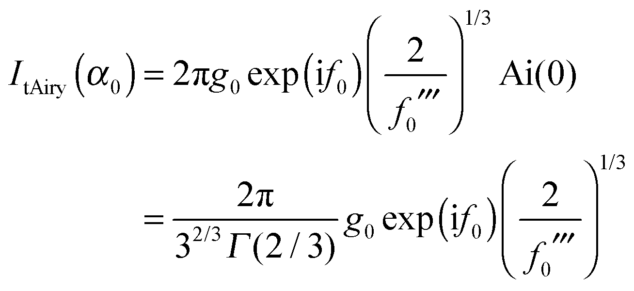
In this section, we examine the 2Hankel approximation for the limiting case α → α0 and ask the question: Do we obtain the transitional Airy approximation (4) in this limit? In eqn (34), (35), (37), (38) and (40) we evidently have to express g1, f1, f1′′, f1′′′, A1 and g2, f2, f2′′, f2′′′, A2 in terms of their values at x0 rather than at x1 and x2. Now for α → α0, we have x1 ≈ x0 ≈ x2 and to extract the limiting behaviour we approximate f(α;x) by its 3-jet at x0, as given by eqn (3) or (6).
When the approximation (3) is valid for f(α;x), the two real stationary phase points, x1 ≤ x2, are the roots of
| (x − x0)2 = −2f0′/f0′′′ | (42) |
Since x1 and x2 are assumed to be real in eqn (42), we must have f0′ ≤ 0 (also recall from Section IIA that f0′′′ > 0). We can write for the two roots
 | (43) |
 | (44) |
| f′′(α;x) = f0′′′(x − x0) |
| f′′′(α;x) = f0′′′ |
It follows that for x = x1
where eqn (43) and (44) have been used. We then find from the definitions (37) and (40) that
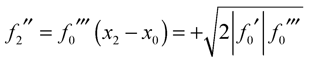
To obtain f1 and f2 we again use eqn (3) together with eqn (43) and (44). The results are
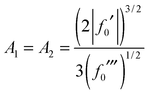
| f1 = f0 + A1 |
| f2 = f0 − A2 |
 | (45) |
Thus we have demonstrated that the 2Hankel approximation contains both limiting cases presented in Section IIB.
III. Derivation of the 6Hankel approximation for rainbow and glory scattering
IIIA. Introduction
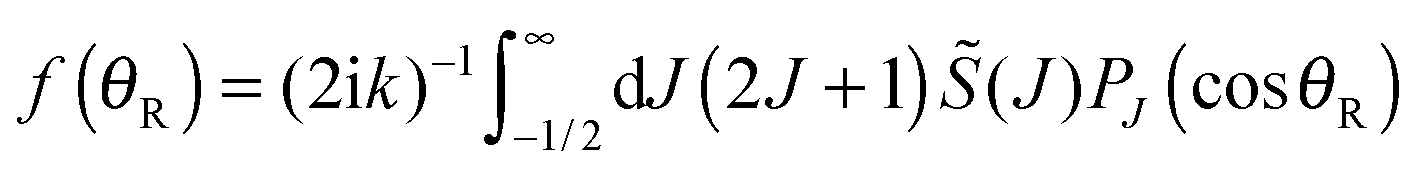
Our starting point is the expansion for the scattering amplitude, f(θR), in a basis set of Legendre polynomials. We write the resulting partial wave series (PWS) in the form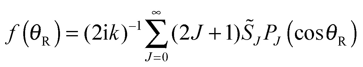 | (46) |
![[S with combining tilde]](https://www.rsc.org/images/entities/i_char_0053_0303.gif) J is the Jth modified scattering matrix element, and PJ(•) is a Legendre polynomial of degree J. In order to keep the notation simple, the label, vi, ji, mi → vf, jf, mf for the initial and final states, has been omitted from f(θR) and J, as has the label, vi, ji, from k. Here v, j, m are vibrational, rotational and helicity quantum numbers respectively, with mi = mf = 0 in our case.
J is the Jth modified scattering matrix element, and PJ(•) is a Legendre polynomial of degree J. In order to keep the notation simple, the label, vi, ji, mi → vf, jf, mf for the initial and final states, has been omitted from f(θR) and J, as has the label, vi, ji, from k. Here v, j, m are vibrational, rotational and helicity quantum numbers respectively, with mi = mf = 0 in our case.
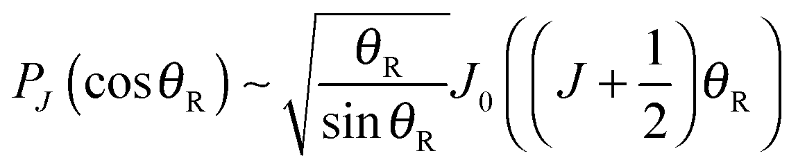
We now introduce standard semiclassical approximations into the PWS (46) to convert it into an oscillating integral.3,4Firstly, we transform the PWS into a Poisson series and retain the leading (m = 0) term; this assumes all the stationary phase points lie in (−π, +π), which is the case for our application – see Section IIIB. We have
 | (47) |
(J) is the continuation of the set of values, {J}, from integer to real values of J and PJ(cos![[thin space (1/6-em)]](https://www.rsc.org/images/entities/char_2009.gif) θR) is now a Legendre function of the first kind. Secondly, we introduce the Hilb approximation to express the Legendre function in terms of a Bessel function, J0(•), of order zero45,46
θR) is now a Legendre function of the first kind. Secondly, we introduce the Hilb approximation to express the Legendre function in terms of a Bessel function, J0(•), of order zero45,46The Hilb approximation has an error, O(J−3/2), which is uniform for θR ∈ [0, π − ε] with ε > 0, We obtain
Thirdly, we express the Bessel function as a sum of two Hankel functions47
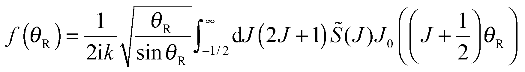
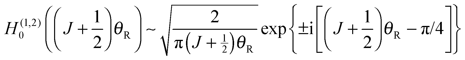
| J0(x) = ½[H(1)0(x) + H(2)0(x)] | (48) |
| f(θR) = f(−)(θR) + f(+)(θR) |
 | (49) |
 | (50) |
 | (51) |
 | (52) |
| exp{±i[(J + ½)θR − π/4]}exp{∓i[(J + ½)θR − π/4]} = 1 |
which implies that the expressions in double braces,
 , are relatively slowly varying with respect to J.
Remark: As in our previous work,3,4,6 we use “∓” to indicate nearside/farside in the semiclassical theory and reserve “N/F” for nearside/farside decompositions in the PWS theory.
The fourth step is the asymptotic evaluation of the oscillatory integrals (50) and (52) using the theory developed in Section II. To do this we must first examine the general properties of (J) for our application. This is done next.
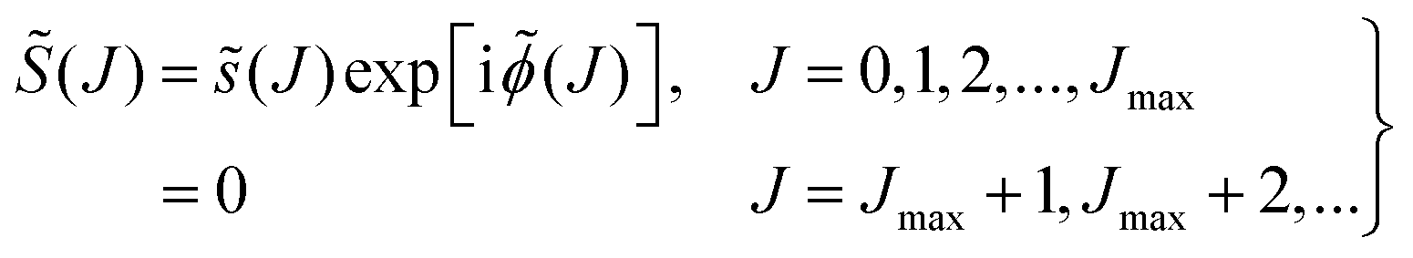
IIIB. Properties of ![[S with combining tilde]](https://www.rsc.org/images/entities/h3_i_char_0053_0303.gif) (J)
(J)
Fig. 2 illustrates the properties of (J) for the J-shifted Eckart model defined in Section IV. In particular, Fig. 2(a) and (b) display |(J)| and arg(J) versus J respectively, whilst Fig. 2(c) is a plot of the quantum deflection function versus J, which is defined byFor eqn (50) and (52), the stationary phase points are the roots of
![[capital Theta, Greek, tilde]](https://www.rsc.org/images/entities/i_char_e134.gif) (J) ∓ θR = 0 (J) ∓ θR = 0 |
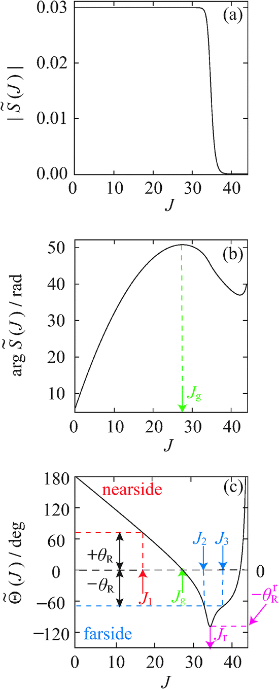 | ||
| Fig. 2 S matrix data for the J-shifted Eckart parameterization. The values of the parameters are given in Section IVB. (a) |(J)| versus J. (b) arg (J)/rad versus J. The maximum of the arg (J)/rad curve defines the glory angular momentum variable, Jg, which is indicated by a green dashed line and arrow. (c) (J)/deg versus J. The red dashed lines and arrow indicate + θR and J1 = J1(θR) for the nearside scattering. The blue dashed lines and arrows indicate −θR, as well as J2 = J2(θR) and J3 = J3(θR) for the farside scattering. Also shown is the rainbow angular momentum variable, Jr, which is located at the minimum of the (J)/deg curve, where (Jr) = −θrR (pink arrow and dashed line respectively), together with Jg, which satisfies the equation (Jg) = 0 (green arrow). | ||
IIIC. Nearside scattering
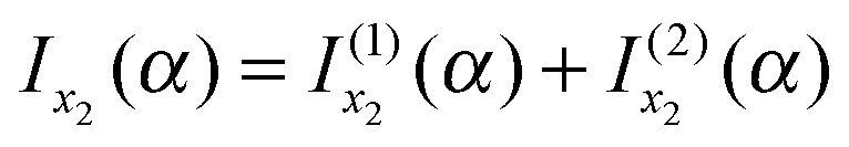
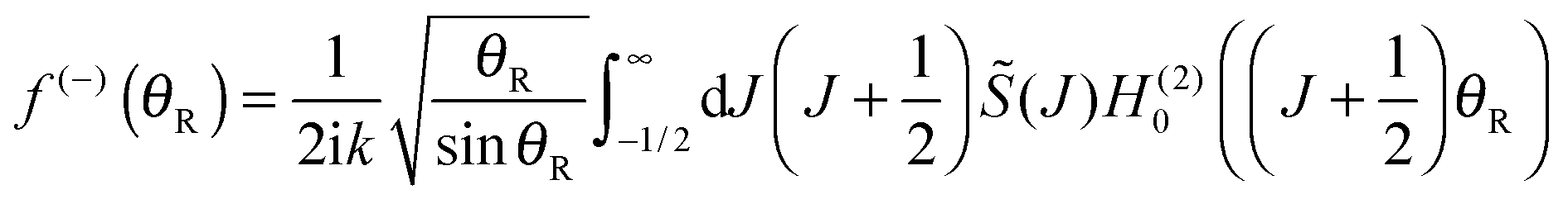
Fig. 2(c) shows there is a single real root to(J) = +θR, which we denote by J1 ≡ J1(θR). The asymptotic theory developed in Section IIC.3 applies, in particular eqn (29).
We make the following identifications between eqn (1) and (50)
| x = J, x1 = J1, α = θR |
| f(α;x) = arg (J) − (J + ½)θR + π/4 |
| f′(α;x) = (J) − θR |
| f′′(α;x) = ′(J) |
| f′′′(α;x) = ′′(J) |
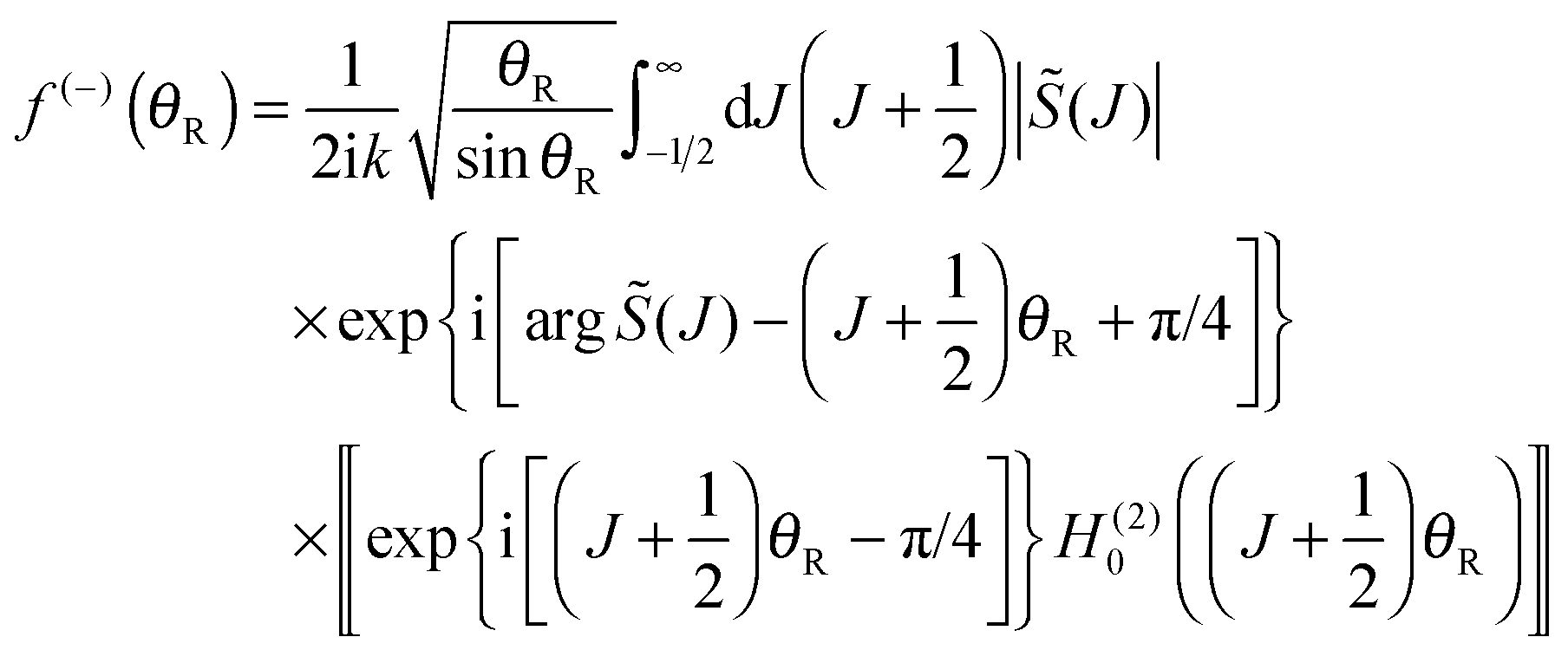
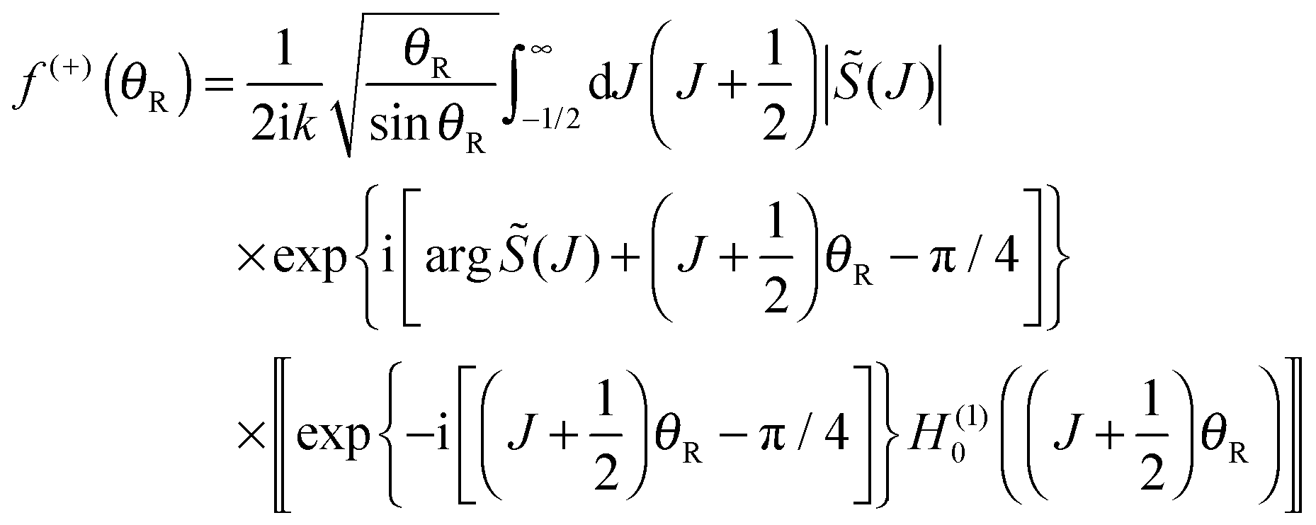
Note that the phase has a linear dependence on θR, namely, −(J + ½)θR. Then from eqn (28), (29) and (50), we can write for the nearside subamplitude to the 6Hankel approximation
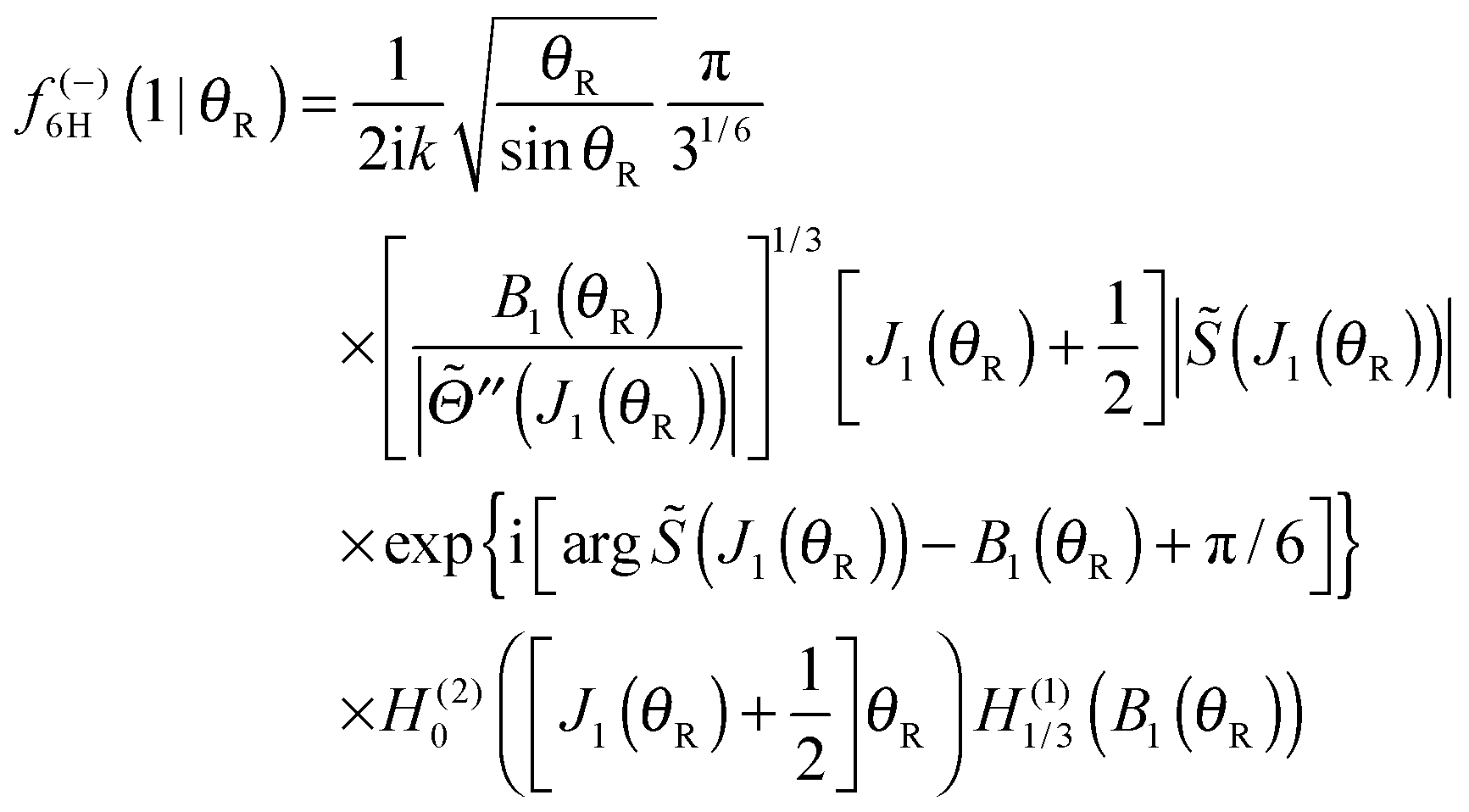 | (53) |
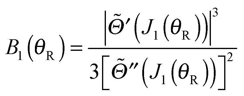 | (54) |
IIID. Farside scattering
Perusal of Fig. 2(c) shows there are two real roots to(J) = −θR, which we denote J2 ≡ J2(θR) and J3 ≡ J3(θR) with J2 ≤ J3. At the rainbow angle, θR = θrR, J2 and J3 coalesce to Jr, the value of the rainbow angular momentum variable; we then have, (Jr) = −θrR. For the farside scattering, the asymptotic theory developed in Section IIC.4 applies and in particular we can use the 2Hankel approximation.
We make the following identifications between eqn (1) and (52)
| x = J, x1 = J2, x2 = J3, α = θR |

| f(α;x) = arg (J) + (J + ½)θR − π/4 |
| f′(α;x) = (J) + θR |
| f′′(α;x) = ′(J) |
| f′′′(α;x) = ′′(J) |
Note that the phase has a linear dependence on θR, namely, +(J + ½)θR. Then from eqn (34), (35), (37), (38), (40) and (52) we have for the two farside subamplitudes which contribute to the 6Hankel approximation
 | (55) |
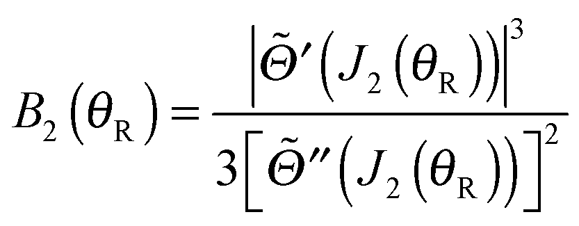 | (56) |
 | (57) |
 | (58) |
IIIE. 6Hankel approximation
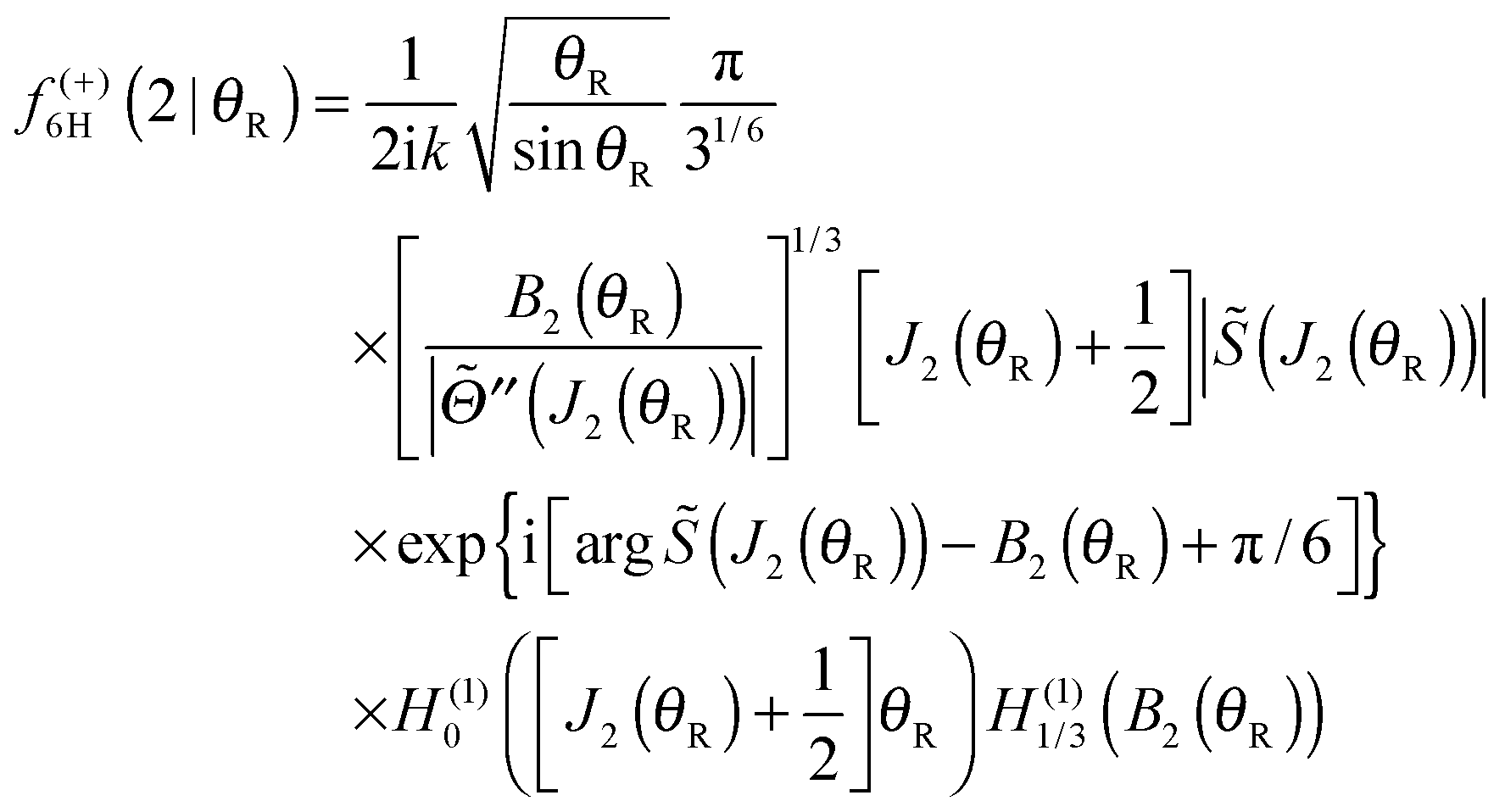
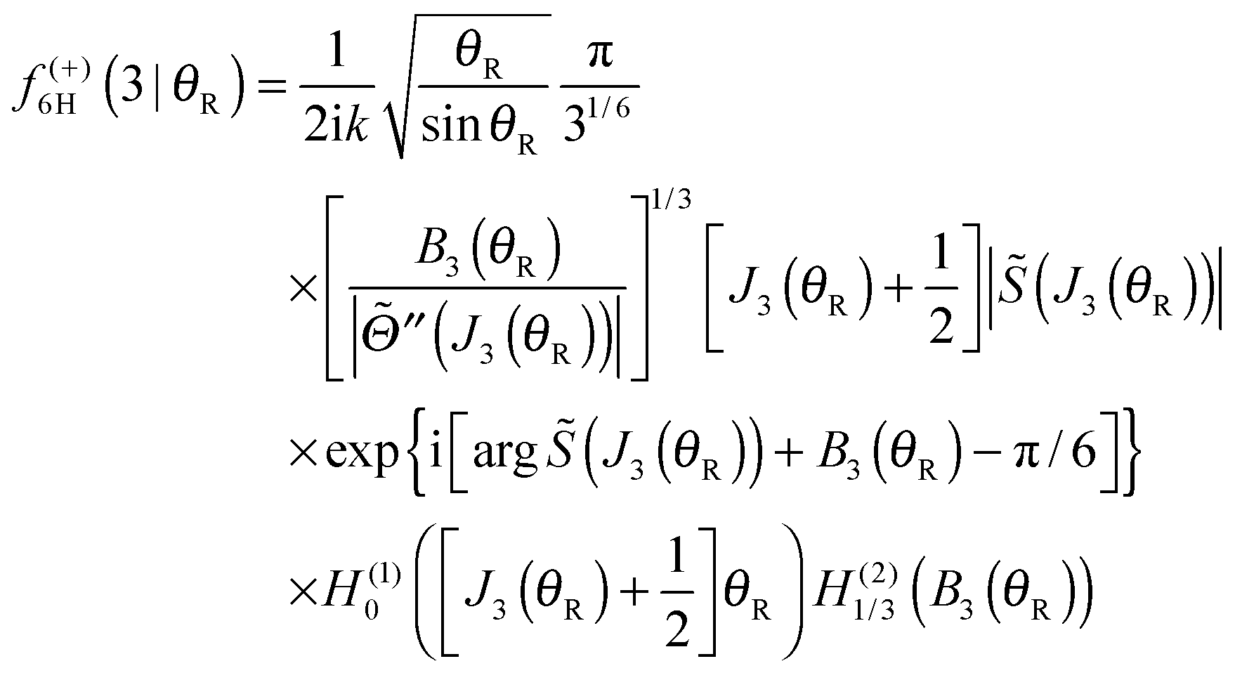
The 6Hankel approximation for the full scattering amplitude is then obtained by summing the subamplitudes (53), (55) and (57)| f6H(θR) = f(−)6H(1|θR) + f(+)6H(2|θR) + f(+)6H(3|θR) | (59) |
The corresponding DCS is
| σ6H(θR) = |f6H(θR)|2 | (60) |
Eqn (59) is the 6Hankel approximation that was written down without proof in our recent paper with Zhang.6 We see that it contains six Hankel functions, three of order zero, H(1,2)0(•), and three of order 1/3, H(1,2)1/3(•).
Note that the farside subamplitudes (55) and (57) are only valid on the bright side of the rainbow angle, where the two roots of (J) = −θR are real. Thus in our calculations in Section V, we will only apply the full 6Hankel approximation (59) for 0 < θR < θrR.
When the arguments of the Hankel functions in eqn (53), (55) and (57) are large, we can substitute the asymptotic results (18) and (19) with ν = 0 or 1/3. We then obtain the following expressions for the subamplitudes, which constitute the primitive semiclassical approximation (PSA):
 | (61) |
 | (62) |
 | (63) |
IIIF. The limit θR → θrR: farside rainbow scattering
When θR → θrR, f(+)6H(2|θR) + f(+)6H(3|θR) becomes numerically unstable because of subtractive cancellation. This arises because′(J2(θR)) → 0 and ′(J3(θR)) → 0 as the rainbow angle is approached, and the asymptotic limits (41) apply to the H(1)1/3(Bi(θR)) with i = 1 and 2. We examined this limit in Section IIC.5, and showed that the 2Hankel approximation contains the transitional Airy approximation (45) [or eqn (4)] when α → α0. We can apply this result to the farside scattering, as given by eqn (55) and (57). Making the identifications| x = J, x0 = Jr, α = θR, α0 = θrR |
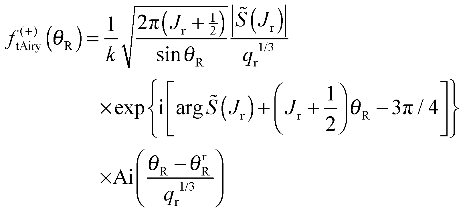 | (64) |
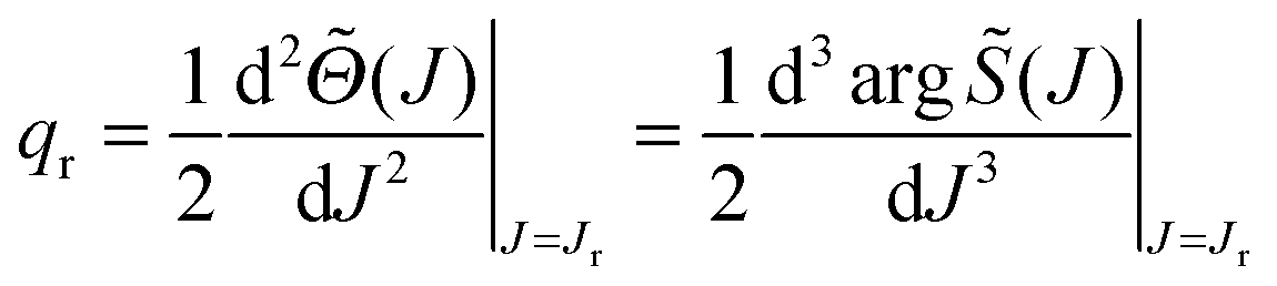
The approximation (64) is equivalent to replacing (J) by its 2-jet at Jr, namely
| jJr2(J) = −θrR + qr(J − Jr)2 |
Eqn (64) has the advantage that it can be used on both the bright side, θR < θrR, and the dark side, θR > θrR, of the rainbow, as well as at θR = θrR.
Remarks:
• In a systematic semiclassical notation,4,6eqn (64) is written as SC/F/tAiry, or tAiry for short.
• When the tAiry subamplitude (64) is used to calculate the DCS, we must also include the contribution from the nearside scattering. We use the SC/N/PSA subamplitude of eqn (61)–(63) for this purpose.
• It is known that the tAiry subamplitude is a special case of the more general uniform Airy approximation, as derived in ref. 4 and 6. In a systematic notation,4,6 it is described as SC/F/uAiry, or uAiry for short.
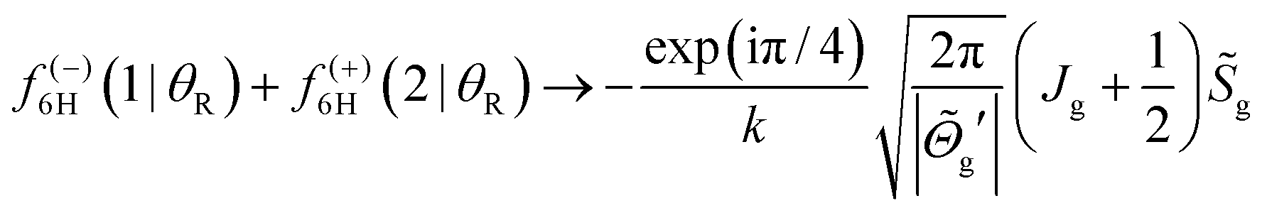
IIIG. The limit θR → 0: glory scattering
Finally we must examine the glory limit, θR → 0, for f(−)6H(1|θR) + f(+)6H(2|θR). In eqn (53) and (55), we note the following limits as θR → 0, for i = 1 or 2;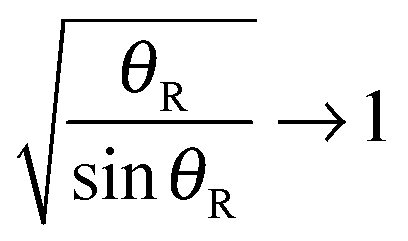
| Ji(θR) → Ji(0) ≡ Jg, |
| ′(Ji(θR)) → ′(Ji(0)) = ′(Jg) ≡ g′ |
| ′′(Ji(θR)) → ′′(Ji(0)) = ′′(Jg) ≡ g′′ |
| Bi(θR) → Bi(0) ≡ Bg |
| (Ji(θR)) → (Ji(0)) = (Jg) ≡ g |
| H(1)1/3(Bi(θR)) → H(1)1/3(Bi(0)) ≡ H(1)1/3(Bg) |
We can use the above limits and the identity (48) to deduce that in the limit θR → 0
| H(2)0([J1(θR) + ½]θR) + H(1)0([J2(θR) + ½]θR) → 2J0(0) = 2 |
We then obtain
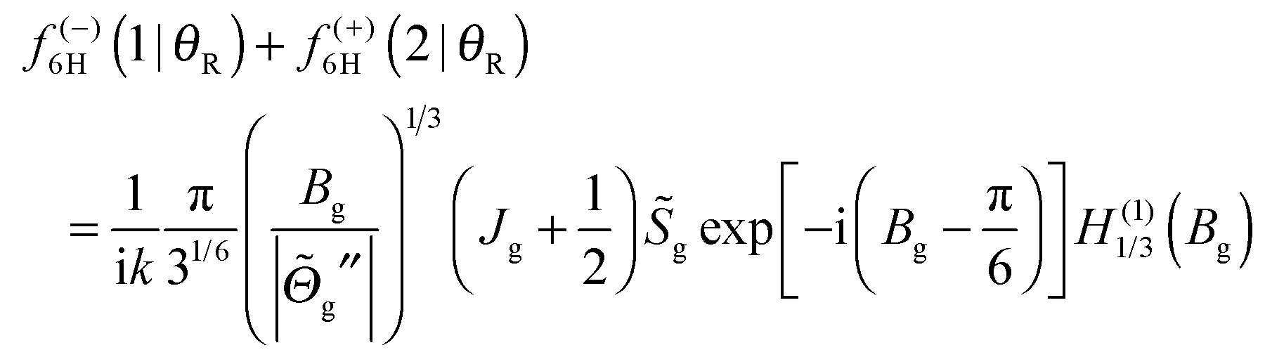 | (65) |
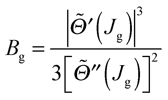 | (66) |
′′(Jg) to be very small in magnitude; hence from eqn (66), we conclude that Bg ≫ 1, and so can use the asymptotic approximation (18) with ν = 1/3 in eqn (65). We obtain for the limit θR → 0which is recognized as the semiclassical transitional approximation (STA) at θR = 0, as given by eqn (14) of ref. 3 or eqn (29) of ref. 7.
Remarks:
• The contribution from f(+)6H(3|θR) to the scattering at θR ≈ 0 is very small in our application in Section V. It has been neglected in the above derivation.
• f(−)6H(1|θR) and f(+)6H(2|θR) become large in magnitude as θR → 0, but their sum f(−)6H(1|θR) + f(+)6H(2|θR) is much smaller. This implies the 6Hankel approximation becomes numerically unstable as θR → 0.
• The STA is a special case of the uniform semiclassical approximation (USA) for forward glory scattering which was derived and discussed in ref. 3 and 7. However, in this paper we will use the more explicit name, uniform Bessel approximation, and use the abbreviation, uBessel.
IIIH. Discussion
We note the following:• The 6Hankel approximation (59) is generic. This means it is applicable to numerous chemical reactions at numerous collision energies (in principle, an infinite number of cases) which have S matrix elements that are analogous to those in Fig. 2.
• The 6Hankel approximation (59) is uniform for both rainbow and glory scattering, with the advantage that the contributions from all three roots J1, J2, J3 appear separately. In contrast, in the standard semiclassical approach, it is necessary to apply two different theories: the uniform rainbow theory (SC/F/uAiry or uAiry),4,6 which involves the pair of roots, J2 and J3; and the uniform glory theory (uBessel),3,7 which involves the pair J1 and J2.
• The 6Hankel approximation (59) has the disadvantage that it involves third derivatives of arg (J); these can be difficult to calculate accurately for numerical input data. Moreover in practical applications, these third derivatives can change sign. In contrast, the uAiry and uBessel theories involve just the second derivatives.
• The 6Hankel approximation (59) has the disadvantage that it becomes numerically unstable for θR → 0 and for θR → θrR, in particular for numerical {J} that possess errors. These problems can be overcome by using the STA for glory scattering and the tAiry approximation for rainbow scattering.
• The 6Hankel formula for the DCS is a generalization to reactive scattering of a result given by Miller for elastic collisions. In particular, if we set in eqn (53)–(60), |(J)| → 1 and arg (J) → 2δ(J), where δ(J) is the elastic phase shift, then, after considerable algebraic manipulations, we obtain for σ6H(θR) the result quoted by Miller [eqn (6) of ref. 9]. One difference is that Miller assumes the Wentzel–Kramers–Brillouin approximation for δ(J), whereas our derivation shows that this assumption is not necessary.
IV. J-shifted Eckart parameterization and the values of its parameters
This section defines the J-shifted Eckart parameterization for(J) in Section IVA, whilst Section IVB gives the values of its parameters that are used in our DCS computations in Section V.
IVA. J-shifted Eckart parameterization
Sokolovski introduced the J-shifted Eckart parameterization for(J) in order to model the DCS for the state-selected H + D2 → HD + D reaction; in particular to mimic a resonance near the reaction threshold.10,48 It has subsequently been found to be very useful for understanding the dynamics of chemical reactions.11,48,49 The J-shifted Eckart parameterization is based on the exact quantum solution for a particle of reduced mass μ transmitted by a symmetric Eckart potential, W0/cosh2(s/s0), where s is a reaction coordinate, s0 is a reference distance and W0 is the height of the energy barrier. The following formulae define this parameterization:where
![[small phi, Greek, tilde]](https://www.rsc.org/images/entities/i_char_e0e2.gif) (J) = aJ2 + bJ (J) = aJ2 + bJ |
In addition
• N = scaling factor (dimensionless).
•  (dimensionless because of the following definition).
• ε = ℏ2/(2μs02) (dimensions of energy).
• 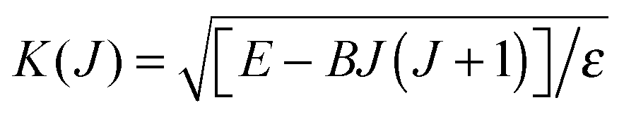 (dimensionless). In this equation, E is the total energy and B is the rotational constant for the triatomic complex. The term BJ(J + 1) represents the J-shifted approximation, because it introduces a J dependence into the mathematically one-dimensional Eckart barrier.
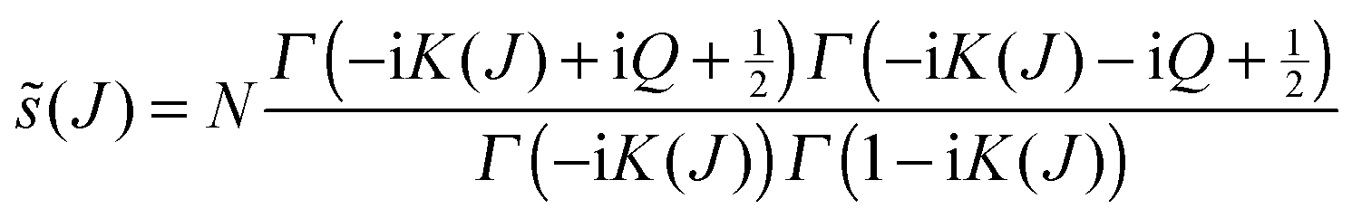
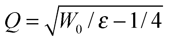
• K(J) has two branch points at real values of J, which are the roots of E − BJ(J + 1) = 0. The larger root is located at 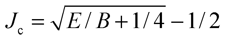 . The integer Jmax is then defined by Jmax = Floor(Jc). It follows that K(Jmax) is real and K(Jmax + 1) is purely imaginary. In our application in Section V, we have Jmax ≫ 1.
IVB. Parameter values for the J-shifted Eckart parameterization
We used the following values for the parameters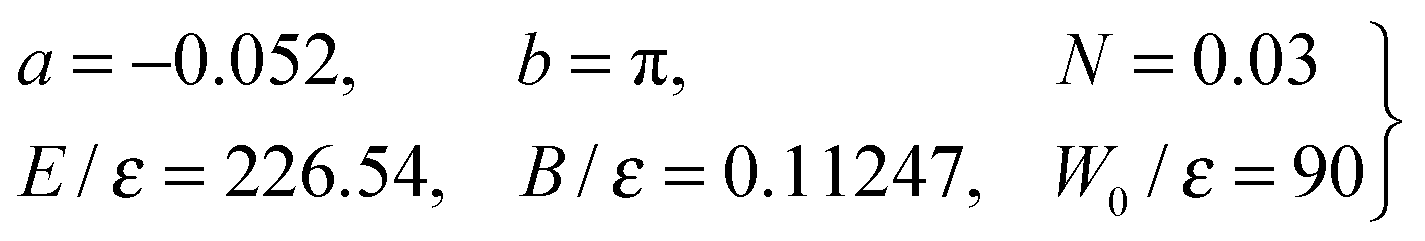 | (67) |
(J)|, arg (J) and (J) versus J respectively have already been shown and discussed in Fig. 2(a), (b) and (c) respectively. In Section V, we will require the position of the leading Regge pole (n = 0) in the first quadrant of the complex angular momentum plane for the J-shifted Eckart potential with the parameter values (67). It is obtained from the poles of Γ(−iK(J) + iQ + 1/2) and is given by J0 = 34.4 + 1.21i, which corresponds to a life-angle of 1/(2ImJ0) = 0.415 rad = 23.8°.
Remark: the parameter values (67) are based on the “standard values” employed for the H + D2 reaction,10,11 which have B/ε = 0.12247 and W0/ε = 150. However, the standard values result in θrR = 24.0° at Jr = 25.2, which only allows a test of the 6Hankel approximation over a relatively small range of angles. Changing B/ε to 0.11247 and W0/ε to 90 gives θrR = 109.2° at Jr = 34.5, which permits the semiclassical approximations to be tested over a wider range of θR.
V. Results for the J-shifted Eckart parameterization
This section presents our results for the angular scattering in Section VA, whilst Section VB reports a nearside–farside (NF) analysis of the (dimensionless) DCS, as well as a NF analysis for the local angular momentum (LAM). All the semiclassical DCSs are defined as the square modulus of the corresponding scattering amplitude.VA. Dimensionless differential cross sections
Fig. 3 plots, on a linear scale, the dimensionless differential cross section (dDCS), k2σ(θR), versus θR for the PWS, where it is compared with the uAiry + SC/N/PSA, uBessel and 6Hankel approximations for θR < θrR. When θR ≥ θrR, the dDCS for the tAiry + SC/N/PSA approximation is drawn. For consistency with ref. 4, the tAiry subamplitude includes the first correction term to eqn (64), even though it makes only a small contribution to the dDCS [see eqn (33) of ref. 4]. Notice that the uAiry + SC/N/PSA curve diverges as θR → 0°, the uBessel curve diverges as θR → θrR, and the tAiry + SC/N/PSA curve diverges as θR → 180°.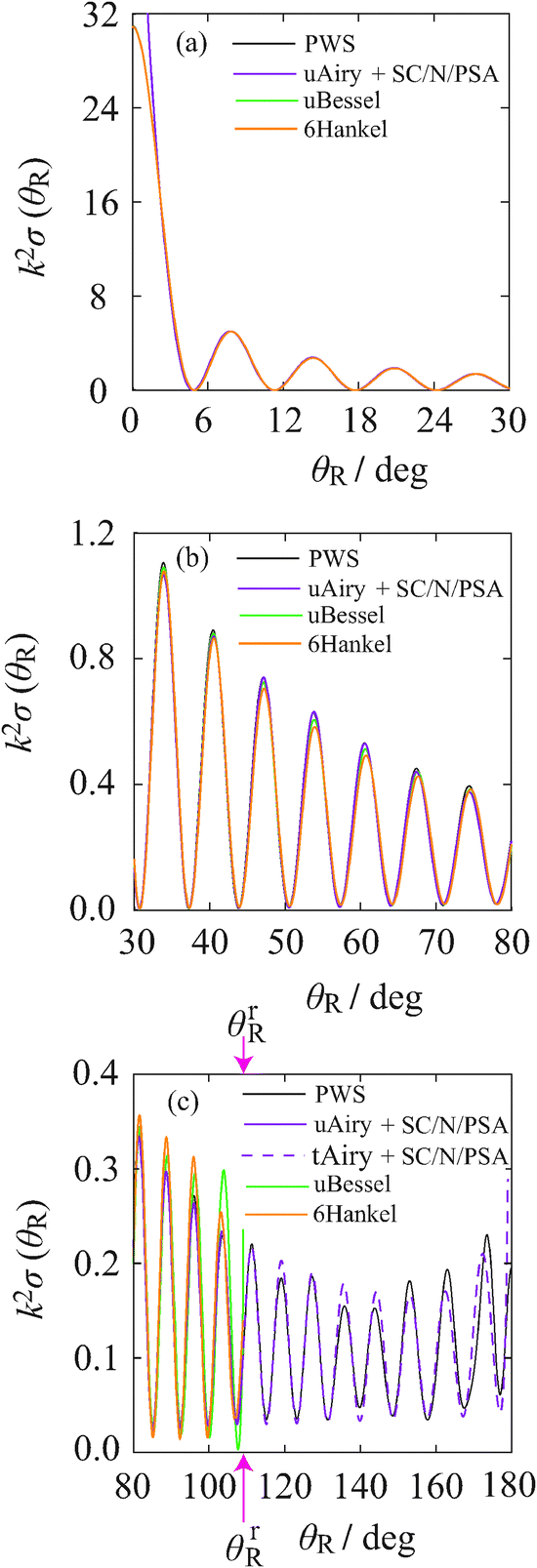 | ||
| Fig. 3 Linear plot of the dimensionless angular distribution, k2σ(θR) versus θR. Black solid curve: PWS. Purple solid curve: uAiry + SC/N/PSA. Purple dashed curve: tAiry + SC/N/PSA. Green solid curve: uBessel. Orange solid curve: 6Hankel. (a) 0° ≤ θR ≤ 30°. The uAiry + SC/N/PSA curve diverges as θR → 0°. (b) 30° ≤ θR ≤ 80°. The PWS and uAiry + SC/N/PSA curves are almost coincident for θR ≳ 35°. (c) 80° ≤ θR ≤ 180°. The pink solid arrows indicate the rainbow angle, θrR = 109.2°. The uBessel curve diverges as θR → θrR. The tAiry + SC/N/PSA approximation is used for θR ≥ θrR; it diverges as θR → 180°. | ||
Fig. 3(a) shows the range, 0° ≤ θR ≤ 30°. We see that the PWS, uBessel and 6Hankel dDCSs agree to graphical accuracy, as does the uAiry + SC/N/PSA dDCS for θR ≳ 2°. The same is mostly true for the range, 30° ≤ θR ≤ 80°, displayed in Fig. 3(b), except near the maxima of the diffraction oscillations.
For 80° ≤ θR ≤ θrR, Fig. 3(c) shows that the uAiry + SC/N/PSA curve generally agrees best with the PWS dDCS, with the uBessel and 6Hankel dDCSs being less accurate. This last result can be traced back to the 2Hankel approximation, which is generally less accurate than the uAiry approximation for the cuspoid test integrals in the Appendix. For θR ≳ θrR, the agreement between the PWS and tAiry + SC/N/PSA curves is satisfactory. As expected, the discrepancies between these two curves generally increases as we move further into the dark side of the rainbow.
Notice that the rainbow does not possess any supernumerary rainbows in the angular scattering; rather it is an example of a “broad rainbow”.4,6,50
VB. Nearside–farside analyses
The NF decomposition of the PWS for f(θR) is given by ref. 3, 4, 6, 11, 13–17 and 19–24| f(θR) = f(N)(θR) + f(F)(θR) | (68) |
 | (69) |
 | (70) |
| σ(N,F)(θR) = |f(N,F)(θR)|2 | (71) |
In practice, we resum the PWS (46) three times (r = 3) before carrying out the NF decomposition because it is known this helps “clean” the N and F unresummed dDCSs and LAMs of unphysical structure.21–24 We then write PWS/N/r = 3 and PWS/F/r = 3 for the N and F resummed subamplitudes respectively. Totenhofer et al.24 have presented a detailed account of resummation theory for a Legendre PWS; this theory is not repeated here.
Fig. 4(a) reports a NF analysis of the PWS dDCS. We see that the reaction is N dominant, although the PWS/F/r = 3 dDCS is always significant, becoming increasingly important upon moving to smaller scattering angles. This results in pronounced diffraction oscillations in the full dDCS, which arise from interference between the N and F subamplitudes.
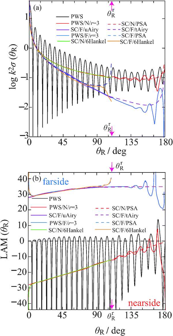 | ||
| Fig. 4 Nearside–farside analyses for the dimensionless logarithmic angular distribution and the Local Angular Momentum. Black solid curve: PWS. Red solid curve: PWS/N/r = 3. Red dashed curve: SC/N/PSA. Solid purple curve: SC/F/uAiry. Purple dashed curve: SC/F/tAiry. Blue solid curve: PWS/F/r = 3. Blue dashed curve: SC/F/PSA. Green solid curve: SC/N/6Hankel. Orange solid curve: SC/F/6Hankel. The pink solid arrows indicate the rainbow angle, θrR = 109.2°. (a) Full and NF logk2σ(θR) versus θR. (b) Full and NF LAM(θR) versus θR. | ||
The PWS results in Fig. 3 for the dDCS, allowed us to test the accuracy of the semiclassical approximations. This is not the case for Fig. 4, because it is known that the NF PWS decomposition of eqn (68)–(71) is not unique: there is no guarantee that it will produce physically useful results.20–24 Rather we use the semiclassical approximations to provide a check on the physical effectiveness of the N, F PWS/r = 3 results. We also recall that the SC/F/6Hankel, SC/F/uAiry, SC/F/PSA and SC/N/6Hankel approximations are only defined for θR < θrR.
Fig. 4(a) plots the N and F dDCSs for the PWS/r = 3, PSA and 6Hankel approximations, and the F dDCSs for the uAiry and tAiry approximations. The agreement between the semiclassical and N, F PWS/r = 3 dDCSs is seen to be generally good. The discrepancies are those expected from our earlier work.3,4,6,11,13–17,19–24 For example, the SC/F/PSA dDCS diverges as θR → θrR, whilst the N and F PWS/r = 3 dDCSs exhibit unphysical oscillations at large angles.
Next we consider the NF analysis of the LAMs.21–24 The full LAM is defined by
 | (72) |
 | (73) |
Fig. 4(b) shows full and N, F LAMs for the PWS/r = 3 and semiclassical approximations. We observe that the LAM information in Fig. 4(b) is consistent with the dDCS information in Fig. 4(a). The discrepancies between the N, F curves are similar to those we have seen previously, e.g., the unphysical oscillations in the N, F PWS/r = 3 LAMs as we approach the backward direction.21–24
We observe that the semiclassical N LAMs decrease in magnitude as θR increases, and are similar to the LAM for the repulsive scattering of two hard spheres,23,24i.e., the N scattering is direct. Next we examine the semiclassical F LAMs. We see that the semiclassical F LAMs are slowly increasing at small θR; then the SC/F/tAiry LAM becomes approximately constant at large angles, where it has the value 34.9. In fact to a very good approximation we have (from ref. 4 and 6)
| LAM(+)tAiry(θR) ≈ Jr + 1/2 = 35.0 |
This behaviour of SC/F/tAiry corresponds in a Regge treatment to decaying (creeping) surface waves that propagate around the reaction zone (see also ref. 52.) When a single Regge pole (n = 0) dominates, we have (from ref. 6 and 27)
| LAM(+)Regge(θR) ≈ Re J0 + 1/2 = 34.9 |
For a broad rainbow, we also expect Jr ≈ Re J0,6,27 which is what we find. If we average over the oscillations in the PWS/F/r = 3 LAM for 100° ≤ θR ≤ 165° we obtain a mean value of 34.5. Thus we have the result

This important result tells us that the PWS, semiclassical and Regge theories are all consistent with each other for the broad rainbow in Fig. 3 and 4(a).
VI. Conclusions
In our recent paper with Zhang,6 we stated without proof the 6Hankel asymptotic approximation for the scattering amplitude, which has the desirable property of being uniform for both a forward glory and a rainbow in the DCS of a chemical reaction. It is also a generic approximation. In this paper we have:• Presented a detailed derivation of the 6Hankel approximation. Our derivation generalizes a method described by Carrier for an oscillating integral with two coalescing real stationary phase points. The generalization uses 3-jets of the phase at the stationary phase points, x1and x2, followed by a discardation of the contributions from the unwanted stationary phase points, u2 and u1. Applying the resulting 2Hankel approximation to the Legendre PWS for the scattering amplitude gives rise to the generic 6Hankel approximation. We also made a test of the accuracy of the 2Hankel approximation by applying it to three cuspoid oscillating integrals.
• Investigated some properties of the 6Hankel approximation. It has the advantage that each root contribution, J1, J2, J3, appears separately in the 6Hankel expression, but has the disadvantage that third derivatives of arg (J) are required. In the limit θR → 0, the 6Hankel approximation reduces to the STA for describing the glory. And in the limit θR → θrR, we obtain the tAiry approximation for rainbow scattering.
• Assessed the accuracy of the 6Hankel approximation for θR < θrR. Using a J-shifted Eckart parametrization of the S matrix, we found that both the 6Hankel and uBessel DCSs agreed well with the PWS DCS at angles close to the forward direction. However using numerical S matrix data, we earlier had found6 the 6Hankel DCS to be less accurate than the uBessel DCS at small angles – probably because of the difficulty of accurately calculating the ′′(Ji). Near the rainbow angle, the 6Hankel DCS generally exhibited greater deviations from the PWS DCS compared to the uAiry + SC/N/PSA DCS. This can be traced back to the 2Hankel approximation, which was generally less accurate than the uAiry approximation for the cuspoid test integrals.
The above trends can be understood in a more general way by remembering that the phases of the semiclassical integrands are not approximated in the uBessel and uAiry approximations – rather exact local one-to-one transformations are made – and only the pre-exponential factors are approximated.3,4,7,8 Whereas, in the 2Hankel and 6Hankel approximations, both the phases and pre-exponential factors are approximated.
Also relevant is the following comment made by Ursell in his last published paper concerning the solution of (water) wave problems:53
“Such a problem is usually solved by applying a sequence of mathematical arguments, and it would be helpful if some or all of the successive steps in this sequence could be given a physical interpretation. In the author's experience this is generally not possible.”
Ursell illustrates his comment by several examples of mathematical steps that do not have a physical interpretation, in particular the use of the exact local one-to-one transformation employed in the method of Chester et al.39 for the uniform asymptotic evaluation of an oscillating integral with two coalescing saddle points. This is also the key transformation used in the derivation of the uAiry approximation.4,8
Appendix: application of the 2Hankel approximation to cuspoid integrals
In this Appendix, we assess the accuracy of the 2Hankel approximation (34) when it is applied to three cuspoid integrals28,29 of the Case A type. We also compare with results from the uniform Airy approximation (uAiry) derived by CM,8 which is based on the technique of Chester et al.39 For a Case A integral, the uniform Airy approximation is given in Section IIIG of CM, namely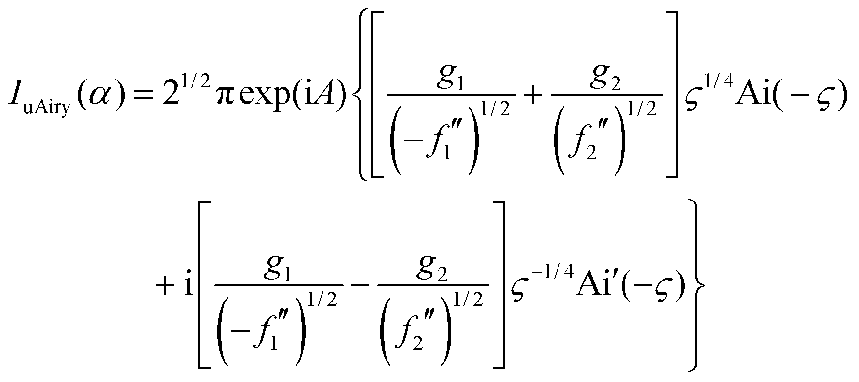 | (A1) |
| A(α) = ½(f1 + f2) |
| ς(α) = [¾(f1 − f2)]2/3 |
Here Ai′(x) means dAi(x)/dx. Note that ς(α) ≥ 0 for real roots. When ς ≫ 1, so the stationary phase points are well separated, the simple stationary phase result (2) is obtained upon replacing Ai(−ς) and Ai′(−ς) by their asymptotic approximations. When ς ≈ 0, so the stationary phase points are close together, the transitional Airy approximation (4) is obtained when f(α;x) is approximated by its 3-jet, as in eqn (3) or (6). For this situation, eqn (A1) for IuAiry(α) becomes an exact result, provided g(x) = 1.
In the following three examples, all the phases are real and have a linear dependence on α of the type, −αx. In all three cases, g(x) = 1. The corresponding oscillating integrals have been calculated numerically by deforming the contour of integration from the real axis into the complex plane as explained in ref. 54–56.
Example 1. Cubic polynomial phase
We write the cubic phase in the form | (A2) |
Example 2. Quintic polynomial phase: an oddoid integral of order two
In this example we choose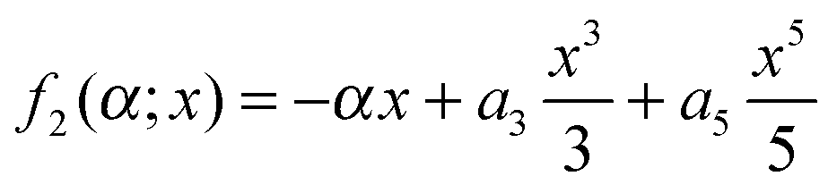 | (A3) |
where the oddoid integral is defined in ref. 29
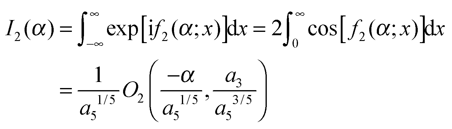
with b1 and b2 real. Hobbs et al.29 have discussed the properties of oddoid (and evenoid) integrals. Now Descartes' Rule of Signs57 tells us that the quartic equation df2(α;x)/dx = 0 for α > 0 has one positive root and one negative root, which coalesce when α = 0. For α < 0, these roots become complex conjugates.
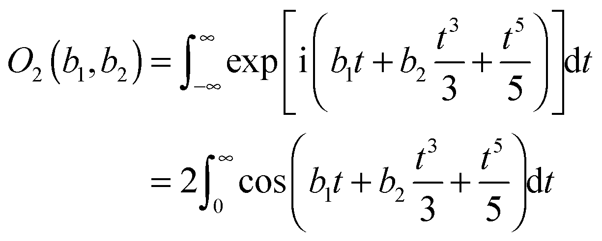
Fig. 5(a) plots I2(α) versus α for the range 0 ≤ α ≤ 15 with phase parameters of a3 = a5 = 5. The oscillatory nature of I2(α) can be clearly seen. Also plotted are the 2Hankel and uAiry approximations as well as the SPA [these curves are also drawn in more detail for α ≤ 5 in Fig. 5(b)]. The SPA is accurate for α ≳ 2 and, as expected, it diverges as α → 0. The 2Hankel approximation becomes systematically smaller than I2(α) for α ≲ 3, until α ≈ 0.15, when the two curves cross. The uAiry approximation agrees closely with I2(α) over the whole range of α.
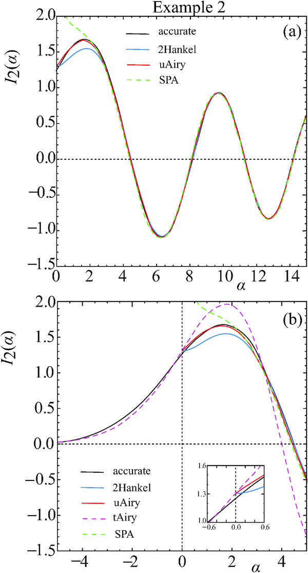 | ||
| Fig. 5 (a) I2(α) and three asymptotic approximations for 0 ≤ α ≤ 15. Black solid curve: I2(α). Red solid curve: uAiry. Blue solid curve: 2Hankel. Green dashed curve: SPA. (b) I2(α) and four asymptotic approximations for −5 ≤ α ≤ 5. Black solid curve: I2(α). Red solid curve: uAiry. Blue solid curve: 2Hankel. Green dashed curve: SPA. Pink dashed curve: tAiry. The inset shows the corresponding curves for −0.6 ≤ α ≤ 0.6 (not SPA). | ||
It was mentioned in Section IIB that the tAiry approximation is also valid for negative α. Fig. 5(b) compares ItAiry(α) with I2(α) for −5 ≤ α ≤ 5. It can be seen that there is good agreement between the two curves for negative α. This finding is very useful since the theory and application of the 2Hankel and uAiry approximations for negative α in practical applications is usually much more difficult than for α > 0. However Fig. 5(b) shows that the tAiry approximation quickly becomes inaccurate for positive α, in particular for the amplitude of the oscillation at α ≈ 2. And this continues to be the case for α > 5 where the positions and amplitudes of the maxima and minima in I2(α) are not reproduced (not shown). At α = 0, the 6Hankel and uAiry approximations become equivalent to the tAiry approximation; this result can be seen visually in the inset to Fig. 5(b). Note that the tAiry approximation is obtained by putting a5 = 0 in the phase (A3). Also from eqn (5) we have
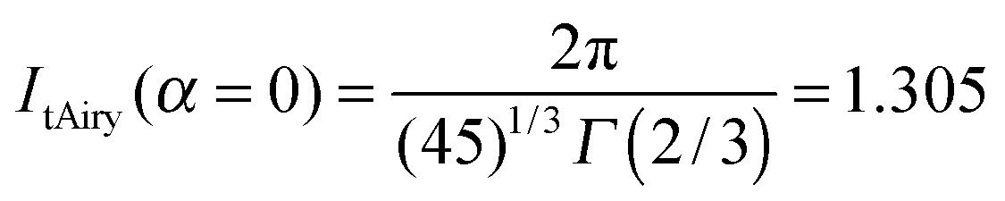
The accurate value for I2(α = 0) is 1.251, so the percentage error in ItAiry(α = 0) is 4.3%.
Example 3. Quintic polynomial phase: A swallowtail integral
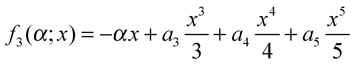
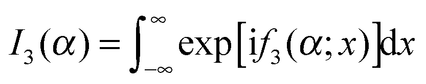
In our third example we choosewith a3 > 0, a4 > 0, a5 > 0 and α ≥ 0. (Again we also let α < 0 for the tAiry approximation.) The corresponding oscillating integral
is an example of a swallowtail integral,28,55 which is complex valued in general. Descartes' Rule of Signs57 tells us that the quartic equation df3(α;x)/dx = 0 for α > 0 has one positive root and one negative root, which coalesce at α = 0. For α < 0, these roots become complex conjugates. We have compared I2H(α), IuAiry(α), ItAiry(α) with I3(α) for many values of a3, a4, a5 when 0 ≤ α ≤ 20 [and also −5 ≤ α ≤ 20 for the tAiry approximation]. In general, the accuracy of the asymptotic formulae are similar to that already discussed in Fig. 5 for Example 2, so, we do not display the corresponding graphs.
Acknowledgements
Support of this research by the UK Engineering and Physical Sciences Research Council and a UK Leverhulme Trust Emeritus Fellowship to JNLC is gratefully acknowledged.References
- Tutorials in Molecular Reaction Dynamics, ed. M. Brouard and C. Vallance, RSC Publishing, Cambridge, UK, 2010 Search PubMed.
- D. M. Neumark, A. M. Wodtke, G. N. Robinson, C. C. Hayden and Y. T. Lee, J. Chem. Phys., 1985, 82, 3045 CrossRef CAS.
- J. N. L. Connor, Phys. Chem. Chem. Phys., 2004, 6, 377 RSC.
- C. Xiahou and J. N. L. Connor, J. Phys. Chem. A, 2009, 113, 15298 CrossRef CAS PubMed.
- X. Wang, W. Dong, M. Qiu, Z. Ren, L. Che, D. Dai, X. Wang, X. Yang, Z. Sun, B. Fu, S.-Y. Lee, X. Xu and D. H. Zhang, Proc. Natl. Acad. Sci. U. S. A., 2008, 105, 6227 CrossRef CAS PubMed.
- C. Xiahou, J. N. L. Connor and D. H. Zhang, Phys. Chem. Chem. Phys., 2011, 13, 12981 RSC . In Section VA.4, for “displaced from θR = 10°”, read “displaced from θR = 0°”.
- J. N. L. Connor, Mol. Phys., 2005, 103, 1715 CrossRef CAS.
- J. N. L. Connor and R. A. Marcus, J. Chem. Phys., 1971, 55, 5636 CrossRef CAS; For a commentary, see: J. N. L. Connor, Current Contents: Physical, Chemical and Earth Sciences, 1991, vol. 31, no. 50, p. 10 Search PubMed; J. N. L. Connor, Current Contents: Engineering, Technology and Applied Sciences, 1991, vol. 22, no. 50, p. 10. Also available at http://garfield.library.upenn.edu/classics1991/A1991GR14400001.pdf Search PubMed.
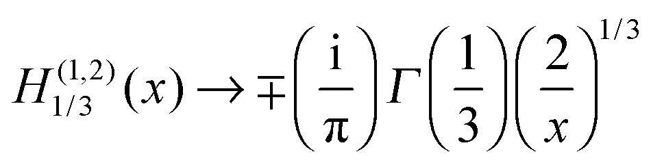
- W. H. Miller, J. Chem. Phys., 1968, 48, 464 CrossRef . In eqn (6), for “
 ”, read “
 ”.
”. - D. Sokolovski, Chem. Phys. Lett., 2003, 370, 805 CrossRef CAS.
- C. Xiahou and J. N. L. Connor, Mol. Phys., 2006, 104, 159 CrossRef CAS.
- J. A. Adam, Phys. Rep., 2002, 356, 229 CrossRef CAS.
- C. Xiahou and J. N. L. Connor, in Semiclassical and Other Methods for Understanding Molecular Collisions and Chemical Reactions, ed. S. Sen, D. Sokolovski and J. N. L. Connor, Collaborative Computational Project on Molecular Quantum Dynamics (CCP6), Daresbury Laboratory, Warrington, UK, 2005, pp. 44–49, ISBN 0-9545289-3-X Search PubMed.
- J. N. L. Connor, X. Shan, A. J. Totenhofer and C. Xiahou, in Multidimensional Quantum Mechanics with Trajectories, ed. D. V. Shalashilin and M. P. de Miranda, Collaborative Computational Project on Molecular Quantum Dynamics (CCP6), Daresbury Laboratory, Warrington, UK, 2009, pp. 38–47, ISBN 978-0-9545289-8-0 Search PubMed.
- X. Shan and J. N. L. Connor, Phys. Chem. Chem. Phys., 2011, 13, 8392 RSC.
- X. Shan and J. N. L. Connor, J. Chem. Phys., 2012, 136, 044315 CrossRef PubMed.
- X. Shan and J. N. L. Connor, J. Phys. Chem. A, 2012, 116, 11414 CrossRef CAS PubMed.
- G. F. Carrier, J. Fluid Mech., 1966, 24, 641 CrossRef . In the Appendix, p. 658: On line 7, for “h(z) = α”, read “h′(z) = α”; on line 17, for “f′′(z0)”. read “h′′(z0)”; on line 26, for eqn (1)”, read “eqn (A1)”; in eqn (A5), for “f′′′(z0)”, read “h′′′(z0)”. On p. 659, in eqn (A6), for “f′′′(z0)”, read “h′′′(z0)”.
- J. N. L. Connor, P. McCabe, D. Sokolovski and G. C. Schatz, Chem. Phys. Lett., 1993, 206, 119 CrossRef CAS.
- P. McCabe and J. N. L. Connor, J. Chem. Phys., 1996, 104, 2297 CrossRef CAS.
- R. Anni, J. N. L. Connor and C. Noli, Phys. Rev. C: Nucl. Phys., 2002, 66, 044610 CrossRef.
- R. Anni, J. N. L. Connor and C. Noli, Khim. Fiz., 2004, 23(2), 6 CAS . Also available at: http://arXiv.org/abs/physics/0410266.
- J. N. L. Connor and R. Anni, Phys. Chem. Chem. Phys., 2004, 6, 3364 RSC.
- A. J. Totenhofer, C. Noli and J. N. L. Connor, Phys. Chem. Chem. Phys., 2010, 12, 8772 RSC.
- J. N. L. Connor, J. Chem. Soc., Faraday Trans., 1990, 86, 1627 RSC.
- D. Sokolovski, J. F. Castillo and C. Tully, Chem. Phys. Lett., 1999, 313, 225 CrossRef CAS.
- J. N. L. Connor, J. Chem. Phys., 2013, 138, 124310 CrossRef CAS PubMed.
- J. N. L. Connor, Mol. Phys., 1976, 31, 33 CrossRef CAS.
- C. A. Hobbs, J. N. L. Connor and N. P. Kirk, J. Comput. Appl. Math., 2007, 207, 192 CrossRef . In eqn (21), in the T5(t,a) expression, for “4at3”, read “5at3”.
- W. H. Miller, J. Chem. Phys., 1970, 53, 3578 CrossRef CAS.
- J. N. L. Connor, Faraday Discuss. Chem. Soc., 1973, 55, 51 RSC.
- J. N. L. Connor, Mol. Phys., 1973, 25, 181 CrossRef.
- J. N. L. Connor, Mol. Phys., 1973, 26, 1217 CrossRef CAS.
- J. N. L. Connor, Mol. Phys., 1973, 26, 1371 CrossRef CAS.
- J. N. L. Connor, Mol. Phys., 1974, 27, 853 CrossRef CAS.
- J. N. L. Connor, Chem. Phys. Lett., 1974, 25, 611 CrossRef CAS.
- D. Sokolovski, J. N. L. Connor and G. C. Schatz, Chem. Phys. Lett., 1995, 238, 127 CrossRef CAS.
- D. Sokolovski, J. N. L. Connor and G. C. Schatz, J. Chem. Phys., 1995, 103, 5979 CrossRef CAS.
- C. Chester, B. Friedman and F. Ursell, Proc. Cambridge Philos. Soc., 1957, 53, 599 CrossRef; Reprinted in Ship Hydrodynamics, Water Waves and Asymptotics, Collected Papers of F. Ursell, 1946–1992, ed. F. Ursell, World Scientific, Singapore, 1994, vol. II, pp. 708–720 Search PubMed; For a commentary, see Ship Hydrodynamics, Water Waves and Asymptotics, Collected Papers of F. Ursell, 1946–1992, ed. F. Ursell, World Scientific, Singapore, 1994, vol. II, p. 570 Search PubMed.
- T. Poston and I. N. Stewart, Taylor Expansions and Catastrophes, Pitman Publishing, London, UK, 1976, p. 13 Search PubMed.
- W. Sanns, Catastrophe Theory with Mathematica: A Geometric Approach, Der Andere Verlag, Osnabrück, Germany, 2000, ch. 3 Search PubMed.
- F. W. J. Olver, in NIST Handbook of Mathematical Functions, ed. F. W. J. Olver, D. W. Lozier, R. F. Boisvert and C. W. Clark, Cambridge University Press, Cambridge, UK, 2010, ch. 9, item 9.6.6. Also available at http://dlmf.nist.gov/, Release 1.0.6 of 2013-05-06 Search PubMed.
- F. W. J. Olver and L. C. Maximon, in NIST Handbook of Mathematical Functions, ed. F. W. J. Olver, D. W. Lozier, R. F. Boisvert and C. W. Clark, Cambridge University Press, Cambridge, UK, 2010, ch. 10, items 10.2.5 and 10.2.6. Also available at http://dlmf.nist.gov/, Release 1.0.6 of 2013-05-06 Search PubMed.
- F. W. J. Olver and L. C. Maximon, in NIST Handbook of Mathematical Functions, ed. F. W. J. Olver, D. W. Lozier, R. F. Boisvert and C. W. Clark, Cambridge University Press, Cambridge, UK, 2010, ch. 10, item 10.7.7. Also available at http://dlmf.nist.gov/, Release 1.0.6 of 2013-05-06 Search PubMed.
- E. Hilb, Math. Z., 1919, 5, 17 CrossRef.
- N. M. Temme, Special Functions: An Introduction to the Classical Functions of Mathematical Physics, Wiley, New York, USA, 1996, p. 160 Search PubMed.
- F. W. J. Olver and L. C. Maximon, in NIST Handbook of Mathematical Functions, ed. F. W. J. Olver, D. W. Lozier, R. F. Boisvert and C. W. Clark, Cambridge University Press, Cambridge, UK, 2010, ch. 10, item 10.4.4. Also available at http://dlmf.nist.gov/, Release 1.0.6 of 2013-05-06 Search PubMed.
- D. Sokolovski and A. Z. Msezane, Phys. Rev. A: At., Mol., Opt. Phys., 2004, 70, 032710 CrossRef.
- P. D. D. Monks, C. Xiahou and J. N. L. Connor, J. Chem. Phys., 2006, 125, 133504 CrossRef CAS PubMed.
- J. N. L. Connor, D. Farrelly and D. C. Mackay, J. Chem. Phys., 1981, 74, 3278 CrossRef CAS.
- R. C. Fuller, Phys. Rev. C: Nucl. Phys., 1975, 12, 1561 CrossRef CAS.
- D. Sokolovski, D. De Fazio, S. Cavalli and V. Aquilanti, Phys. Chem. Chem. Phys., 2007, 9, 5664 RSC.
- F. Ursell, J. Eng. Math., 2007, 58, 7 CrossRef.
- J. N. L. Connor and P. R. Curtis, J. Phys. A: Math. Gen., 1982, 15, 1179 CrossRef.
- J. N. L. Connor, P. R. Curtis and D. Farrelly, J. Phys. A: Math. Gen., 1984, 17, 283 CrossRef.
- N. P. Kirk, J. N. L. Connor, P. R. Curtis and C. A. Hobbs, Comput. Phys. Commun., 2000, 132, 142 CrossRef CAS.
- J. V. Uspensky, Theory of Equations, McGraw-Hill, New York, USA, 1963, paperback version of the 1948 edition, ch. VI, Section 10 Search PubMed.
| This journal is © the Owner Societies 2014 |