L-edge X-ray absorption study of mononuclear vanadium complexes and spectral predictions using a restricted open shell configuration interaction ansatz†
Received
28th June 2013
, Accepted 24th October 2013
First published on 24th October 2013
Abstract
A series of mononuclear V(V), V(IV) and V(III) complexes were investigated by V L-edge near edge X-ray absorption fine structure (NEXAFS) spectroscopy. The spectra show significant sensitivity to the vanadium oxidation state and the coordination environment surrounding the vanadium center. The L-edge spectra are interpreted with the aid of the recently developed Density Functional Theory/Restricted Open Shell Configuration Interaction Singles (DFT/ROCIS) method. This method is calibrated for the prediction of vanadium L-edges with different hybrid density functionals and basis sets. For the B3LYP/def2-TZVP(-f) and BHLYP/def2-TZVP(-f) functional/basis-set combinations, good to excellent agreement between calculated and experimental spectra is obtained. A treatment of the spin–orbit coupling interaction to all orders is achieved by quasi-degenerate perturbation theory (QDPT), in conjunction with DFT/ROCIS for the calculation of the molecular multiplets while accounting for dynamic correlation and anisotropic covalency. The physical origin of the observed spectral features is discussed qualitatively and quantitatively in terms of spin multiplicities, magnetic sublevels and individual 2p to 3d core level excitations. This investigation is an important prerequisite for future applications of the DFT/ROCIS method to vanadium L-edge absorption spectroscopy and vanadium-based heterogeneous catalysts.
Introduction
Vanadium is an important element in the field of solid-state catalysis.1 In particular, vanadium-based catalysts are utilized in a variety of oxidation reactions, including the selective oxidation of methane and methanol, as well as the oxidative dehydrogenation of ethane and propane.2–5 Vanadium is also of critical importance in the industrial synthesis of acrolein, acrylic acid, maleic and phthalic anhydride.6 However, despite extensive research, there are still fundamental aspects of these metal-oxide catalysts that are not well understood. In particular, the nature of the active vanadium species that is involved in the elementary catalytic steps of the above mentioned reactions is still controversially debated, especially in the case of the silica-supported catalysts.7,8 Hence, experimental and theoretical methods that give insight into the local geometric and electronic structures of the active species in the surface are urgently needed. A number of recent studies have attempted to correlate the geometric structure of catalysts with their catalytic performance.6,8–10 In particular, experimental in situ techniques based on vibrational and X-ray absorption spectroscopies have been developed.6,11–15 It has been shown that Near Edge X-ray Absorption Fine Structure (NEXAFS) spectroscopy is a powerful technique to study the electronic and geometric structures of materials in an element specific fashion.16 Moreover, core level spectroscopy is not limited to studies of crystalline bulk materials, but it can be also applied to amorphous matter and is suitable for probing the catalytic surface of bulk materials with sub-monolayer sensitivity.
In terms of a simple one-electron picture, the spectral features arise from the excitation of a core electron to the lowest unoccupied or singly occupied orbitals (LUMOs, SOMOs) of the material under investigation. The relevant excitation processes are governed by the usual dipole- and quadrupole selection rules. Thus, the K-edge spectral region is dominated by 1s → np dipole (and quadrupole) transitions, whereas the L2,3 spectral region mainly corresponds to transitions between the 2p-core orbitals and partially filled or empty nd-based orbitals. Being dominantly based on electric dipole allowed transitions into the metal d-orbitals, transition metal L-edge spectra are typically richly structured. They are, however, also difficult to interpret since in addition to ligand-field and covalency effects, one must consider the spin–orbit coupling (SOC) interaction between the potentially many final state multiplets. The SOC interaction dominates the spectral appearance and is responsible for the splitting into distinct L3 and L2 edges. Therefore, L-edge spectra cannot, in general, successfully be interpreted on the basis of a simple one-electron picture, despite the fact that they contain a wealth of geometric and electronic structure information.16,17 In order to extract this information, an efficient theoretical methodology with substantial predictive capabilities and the minimum number of adjustable parameters is required. First principles calculations within the independent particle hole approximation include multiple scattering18 and TD-DFT19–21 methods. While these methods have been proven to be useful in the interpretation of K-edge spectra, they have shown at best limited success in the case of L2,3-edge spectra. In the case of vanadium oxides, O K-edge XAS in combination with TD-DFT calculations has led to the identification of oxygen sites in different binding environments.11,12,22–24 While the calculation of O K-edge spectra provides rather satisfactory agreement with the experimental spectra, the situation is much more challenging in the case of V-2p core level excitations. Several methods have been discussed for the calculation of transition metal L2,3-edge spectra.25–41 It should be stressed that only the many particle states are probed experimentally. Although in many situations one can come to a satisfactory description of experimental spectra on the basis of quasi-particle (particle/hole) methods, this is, in general, not possible for transition metal L-edge spectra. In fact, the theoretical challenges in this field are severe. In many cases it is necessary to construct approximations to the many multiplets that arise from the 2p53dn+1 configurations as well as the 2p53dnL* charge transfer configurations (where L* represents an empty ligand based orbital). In general, this requires more than singly excited Slater determinants to span the correct space of final states. In order to obtain the correct energetic ordering of these multiplet states in a wavefunction based picture, dynamic correlation effects must be accounted for. Finally, the very strong spin–orbit coupling effects arising from the 2p5 core hole configuration must be dealt with. This will lead to a great deal of mixing between the multiplet states and hence will also lead to a great deal of intensity redistribution. Such problems can be adequately solved either in the framework of molecular jj-coupling (in which SOC is introduced at the level of the one particle orbitals) or molecular Russell–Saunders (LS) coupling (in which SOC is introduced at the level of many particle configuration state functions) schemes. In fact, if followed through to completion, both approaches should yield identical results. However, we should emphasize that this has been proven to be an extremely demanding task for approaches that rely on jj (or intermediate, RS) coupling.26,36–38 We have therefore recently developed a completely different methodology for this purpose by introducing the DFT/Restricted Open shell Configuration Interaction Singles (ROCIS) method.42 It has been shown that this method has predictive accuracy. The heart of the method is based on correlated wavefunction methodology and can be thought as a molecular generalization of the familiar LS coupling scheme. In contrast to highly correlated wavefunction based approaches that are confined to very small systems of only a few atoms, the DFT/ROCIS method can be applied to systems with about 100–200 atoms. Hence, classes of chemical systems ranging from coordination complexes to complex cluster models for solids or catalytic surfaces are computationally accessible using standard hardware. In order to strike the best balance between accuracy and efficiency, the method employs DFT orbitals and is parameterized in order to implicitly account for dynamic electron correlation effects. Dynamic correlation effects are indeed important, as in fact the pure ROCIS method fails in many cases to describe the experimental spectra and overall provides much inferior agreement than ROCIS/DFT.42 Three universal parameters have been introduced for the entire periodic table and have been determined through test calculations on a series of first row transition metal complexes. Excellent performance of the DFT/ROCIS method in predicting the L-edge spectra of mononuclear transition metal complexes, as well as oligonuclear cluster models (containing up to 20 metal centers), has been accomplished in recent studies.42,43
It should be noted that the calculated absolute transition energies carry large but highly systematic errors that arise from shortcomings of the density functionals in the core region, limitations of the one-particle basis set and shortcomings in the accurate modeling of spin-free relativistic effects. Given their highly systematic nature, all of these factors can (for a given basis set and density functional) be taken into account by introducing an element-dependent shift.19,20,44–46 In fact it has been shown that a simple linear regression is sufficient to establish predictive accuracy in the calculated transition energies for any given element. This calibration needs to be carried out with respect to a test set of well-known systems and has already been reported for metal- and ligand K-edges in the framework of scalar relativistic DFT methodology.19,20,44,46 In this work, we present a combined V–L-edge experimental and DFT/ROCIS theoretical study on a series of 16 crystallographically characterized mononuclear vanadium complexes.
Experimental
Test set of vanadium complexes
In order to arrive at a well-defined and reliable calibration of the DFT/ROCIS methodology, we have constructed a library of 16 mononuclear vanadium complexes, which have been crystallographically characterized and span a wide range of oxidation-states and coordination environments. The data set consists of the following compounds (Fig. 1): K2[V(V)O(O2)2C5H4NCOO] (1), K2[V(V)O(O2)2C2H4] (2), [V(V)O2(R,R′L1)], R = Me, R′ = Ph (3), R = H, R′ = Me (4), R = H, R′ = Ph (5), R = H, R′ = 4-O2NPh (6), V(IV)O(acac)2 (7), V(IV)O(acac)2Py (8), V(IV)O(TPP) (9), V(IV)O(HRL2), Me (10), Et (11), Cl (12), V(IV)O(salen) (13), [V(IV)(MeO)L3] (14), V(III)(acac)3 (15), [V(III)(MeOH)L3] (16). The abbreviations L1, L2, L3, acac, salen and TPP stand for oxyoxime,47 tris(2-oxo-3,5-di-tert-butylbenzyl)amine,48 salicylaldoxime,47 acetylacetonato, N, N′ bis(salecylidene)ethylendiamine and 5,10,15,20-tetraphenyl-porphine respectively. Complexes 1, 7, 9, 10, 16–18 were purchased or synthesized according to common published procedures.48,49 V L-edge data for complexes 2–6, 8, 11–15 have been reported previously.47 The BP86/def2-TZVP(-f) optimized structures of the above complexes are presented in Fig. 1.
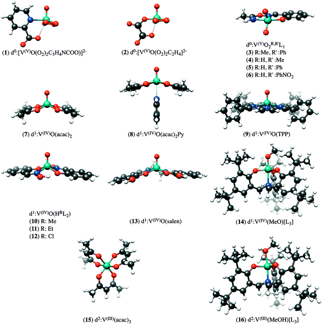 |
| | Fig. 1 Graphical representation of the structure of vanadium complexes investigated in this study. | |
X-ray absorption spectroscopy measurements
In situ NEXAFS measurements were performed at the synchrotron radiation facility BESSY in Berlin (Germany) using the ISISS (Innovative Station for In Situ Spectroscopy) beamline. Pellets of the target compounds, either in pure form or mixed with graphite in order to reduce charging effects, were mounted inside a reaction cell onto a sapphire sample holder approximately 2 mm in front of the first aperture of a differentially pumped electrostatic lens system. An ambient gas pressure of 0.5 mbar oxygen was applied to preserve the sample surfaces against beam-induced reduction. This is potentially a problem for oxygen sensitive compounds but it was found not to be the case for the chosen data set. The home-built electron lens serves as the input system for a modified commercial hemispherical electron analyzer (PHOIBOS 150, Specs-GmbH). Vanadium 2p (L-edge) and oxygen 1s (K-edge) excitation spectra were obtained in total electron yield modes (TEY) by using the electron spectrometer as a detector in order to minimize the contributions from the gas phase to the spectra. Three to four scans on different spots were measured in order to ensure the reproducibility of the reported spectra and the homogeneity of the sample. All reported data correspond to a single scan. Bulk V2O5 was used as an energy calibration reference for the whole data set. The same reference material was used for the complexes studied by Young et al.47 A 2 eV energy shift was applied to the previously published data in order to arrive at a consistently combined dataset. The V L edge spectra are calibrated against the O K-edge TEY data for the π*-resonance of the O2 gas phase (531.0 eV). All spectra are normalized with respect to the highest intensity feature of the V L3 region. However it should be mentioned that the partial overlap between V–L and O–K edges is an issue for V–L-edge spectroscopy. As it will be discussed below in more detail additional data analysis involving background subtraction and quantitative interpretation of signal intensities is not possible without introducing errors. Further details of the experimental methodology have already been presented elsewhere.50
Theory
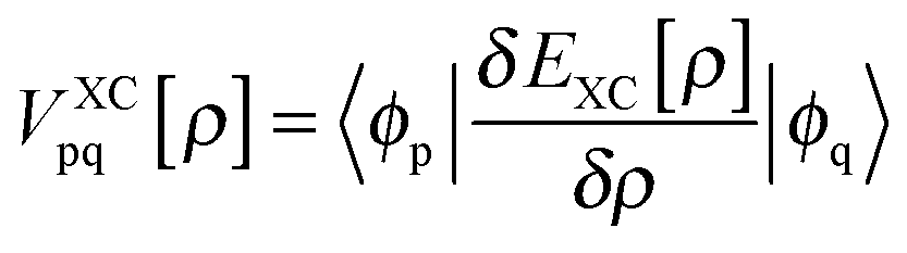
As has been discussed at length recently,42,51 the DFT/ROCIS method can be considered as an ab initio version of a molecular LS coupling scheme. Within the DFT/ROCIS Ansatz, one tries to use the best of two worlds: (i) a good description of the molecular orbitals and metal ligand covalency derived from DFT calculations and (ii) the rigorous multiplet structure and incorporation of SOC effects offered by the configuration interaction approach. In brief, the solution of the self-consistent field (SCF) equations is performed in order to obtain restricted open-shell Kohn–Sham (ROKS) or quasi-restricted (QRO)52 orbitals. Either procedure results in three sets of orbitals: doubly occupied MOs (DOMOs), singly occupied MOs (SOMOs) and empty (virtual) MOs (VMOs). The DOMO and SOMO orbitals are eigenfunctions of the closed- and open shell Kohn–Sham operators with matrix elements:| |  | (1) |
Here, hpq = 〈ϕp|ĥ|ϕq〉 are integrals of the one-electron part of the Born–Oppenheimer Hamilton operator over the molecular orbitals ϕp and ϕq. As usual, labels i, j, k refer to doubly occupied orbitals of the reference determinant, a, b, c, d refer to empty orbitals, t, u, v, w denote singly occupied orbitals and labels p, q, r, s are used for any set of orbitals. The two-electron integrals are stored in Coulomb and exchange matrices of the form:| | 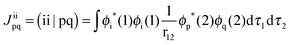 | (2) |
| | 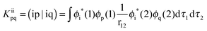 | (3) |
Moreover  denotes matrix elements of the exchange–correlation potential. Both matrices are given in the hybrid density functional form, since hybrid density functionals will be used in all presented DFT/ROCIS calculations. The coefficients cHF and cDF denote the amount of HF exchange and pure density functional related exchange–correlation contribution, respectively. Accordingly, for a HF calculation cDF = 0. The ROCIS method implicitly introduces dynamic electron correlation through three empirical parameters c1, c2 and c3. These parameters are used to scale the Coulomb and exchange integrals in the diagonal of the CI matrix, as well as the off-diagonal CI elements. For example, in the subspace spanned by the singly-excited configuration state functions (CSFs) arising from the single excitation from a DOMO i or j into a VMO a or b, the scaled CI matrix elements become:
| | | HDFT/ROCISia,ia = FC(KS)aa − FC(KS)ii − c1(ii|aa) + 2c2(ii|bb) | (4) |
| | | HDFT/ROCISia,ib = c3{δijFC(KS)ab − δabFC(KS)ij (ii|ab) − 2(ia|ja)} | (5) |
The parameters c1, c2 and c3 were optimized with respect to the test set first row transition metal L-edges and for B3LYP and BHLYP they take the form: c1 = 0.18, c2 = 0.20 and c3 = 0.40 and c1 = 0.21, c2 = 0.30 and c3 = 0.40, respectively.42
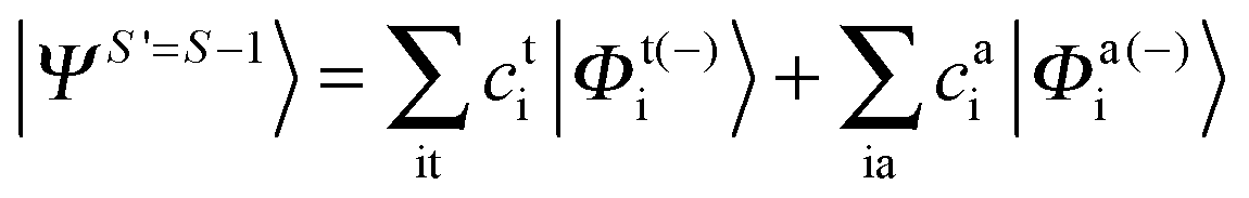
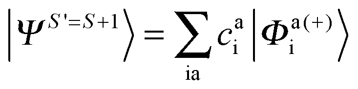
Since we include SOC in the calculation, it is necessary to also calculate excited states that feature spin quantum numbers other than the ground state total spin S. The Ansatz for the three different classes of spin-adapted ROCIS wavefunctions is:
| | 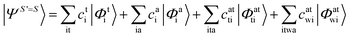 | (6) |
| | 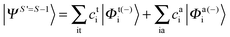 | (7) |
| |  | (8) |
The excited CSF's {|Ψ〉} are generated with the aid of second quantized replacement and spin operators, as explained elsewhere.42 The three blocks of the CI matrix are diagonalized separately for a user specified number of roots.
Spin orbit coupling.
The SOC is calculated using the QDPT (QDPT) on the basis of the non-relativistic roots. The CI procedure leads to excited state wavefunctions of the form 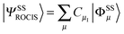 . The upper indices SS denote a many-particle wavefunction with spin quantum number S and spin projection quantum number M = S. Since the BO Hamiltonian is spin free, only one member of a given spin-multiplet (e.g. that with M = S) needs to be calculated. For the treatment of the SOC all |ΨSMI〉 are required (I denotes a given state obtained in the first step of the procedure). Matrix elements over the |ΨSMI〉 functions are readily generated using the Wigner–Eckart theorem, since all (2S + 1) members of the multiplet share the same spatial part of the wavefunction:49
| | | 〈ΨSMI|ĤBO + ĤSOC|ΨS′M′J〉=δIJδSS′δMM′E(s)I + 〈ΨSMI|ĤSOC|ΨS′M′J〉 | (9) |
Since the dimension of the eigenstate basis usually does not exceed a few hundred, this matrix is readily diagonalized thus yielding spin–orbit coupled eigenstates and their energy levels. The SOC operator is approximated by the effective one-electron spin–orbit mean field (SOMF) operator,53–55 which has been shown to provide good results for SOC effects.56,57 If scalar relativistic effects are accounted for, for example by the Douglas–Kroll–Hess Hamiltonian,58–60 appropriate picture change effects are taken into account in the SOC operator.61
Computational details
All calculations were performed with the ORCA suite of programs.62 The BP8663,64 and B3LYP63,65,66 functionals were used together with Grimme's dispersion correction67,68 for geometries/frequencies and electronic properties, respectively. The def2-TZVP basis set of Weigend et al.77 is of triple-ζ quality69 and was used for all the atoms in combination with the matching Coulomb fitting basis for the resolution of identity70,71 (RI, in BP86 calculations). The DFT/ROCIS calculations were performed using the converged restricted RKS or unrestricted UKS Kohn–Sham wavefunctions. For these calculations, the B3LYP and BHLYP density functionals were employed together with the def2-SVP and def2-TZVP(-f) basis sets. Scalar relativistic effects were treated on the basis of the second-order Douglas–Kroll–Hess (DKH)58–60 and ZORA72 methods. In a typical calculation 40–80 roots were calculated to ensure saturation of involved excitations. The absorption spectra were obtained from DFT/ROCIS calculated intensities by applying a Gaussian broadening of 0.8 eV to the calculated transitions. The optimized and crystallographic structures of complexes 1–16 are in very good agreement (selected bond lengths can be found in Table S1 in the ESI†).
Results and analysis
Electronic structure
To a first approximation, qualitative insight into the nature of the dominant 2p → 3d one-electron excitations is provided within a Ligand Field Theory type of analysis (Fig. 2) and is presented below for three characteristic cases, chosen among the sixteen complex sets. The complexes in reference are grouped by the d-electron occupation: d0: K2[V(V)O(O2)2C5H4NCOO] (1), d1: V(IV)O(acac)2 (7) and d2: V(III)(acac)3 (15). In these three vanadium complexes, the vanadium oxidation state ranges between V and III. Upon a 2p-electron excitation the resulting final states belong to the following respective electron configurations: 2p53d1, 2p53d2 and 2p53d3. According to group theory,16 the atomic multiplets that arise from these configuration are 2P ⊗ 2D = 1,3P, 1,3D, 1,3F, 2P ⊗ 3D = 2,4S, 2,4P, 2,4D, 2,4F, 2,3G, 4H and 2P ⊗ 4D = 1,3,5S, 1,3,5P, 1,3,5D, 1,3,5F, 1,3G, 1,3H. These atomic states will further split due to the ligand field and covalency interactions as well as the SOC mixing, to produce a total amount of 60, 270 and 720 molecular magnetic spin sublevels that are characterized by quantum numbers Ms = 0, ±1, Ms = ±½, ±![[/]](https://www.rsc.org/images/entities/char_e0ee.gif) and Ms = 0, ±1, ±2, respectively. They will subsequently be denoted as |0〉,|±1〉,|±½〉,|±〉 and |0〉,|±1〉|±2〉. On the basis of a molecular LS coupling scheme the single electron excitation patterns describing the final states of V(V) and V(IV) in tetragonal and trigonal ligand coordination environments are rather straightforward. In fact, for complexes 1 and 7 the multiplet structure of the final states is dominated by states having the same (S′ = S) or higher (S′ = S + 1) spin multiplicities in comparison to the ground state spin multiplicity S of the system in reference. These states involve mainly excitations of the type DOMO → SOMO and DOMO → VMO. On the other hand, in the case of complex 15 in which the V(III) metal center is coordinated in a distorted Oh environment, the excitation pattern is somewhat more complex. Specifically, the multiplet structure of the final state electronic configuration 2p53d3 has significant contributions from lower multiplicity (S′=S − 1) states. These states involve DOMO → VMO excitations, as well as coupled single electron excitations of the type DOMO → SOMO and SOMO → VMO. Thus, it becomes clear that for all three cases, in order to achieve a quantitative description of the metal L-edge spectra, these excitation patterns should be treated explicitly and within a proper CI scheme including electron correlation and anisotropic covalency. This strategy has been extensively applied to interpret optical and magnetic spectroscopic phenomena.56,57,73 Deconvolution of the calculated spectra can be performed in terms of the magnetic sublevels of the final states, which can be further mapped onto the dominant 2p → 3d excitations in a straightforward and transparent manner, as will be explored in detail below.
and Ms = 0, ±1, ±2, respectively. They will subsequently be denoted as |0〉,|±1〉,|±½〉,|±〉 and |0〉,|±1〉|±2〉. On the basis of a molecular LS coupling scheme the single electron excitation patterns describing the final states of V(V) and V(IV) in tetragonal and trigonal ligand coordination environments are rather straightforward. In fact, for complexes 1 and 7 the multiplet structure of the final states is dominated by states having the same (S′ = S) or higher (S′ = S + 1) spin multiplicities in comparison to the ground state spin multiplicity S of the system in reference. These states involve mainly excitations of the type DOMO → SOMO and DOMO → VMO. On the other hand, in the case of complex 15 in which the V(III) metal center is coordinated in a distorted Oh environment, the excitation pattern is somewhat more complex. Specifically, the multiplet structure of the final state electronic configuration 2p53d3 has significant contributions from lower multiplicity (S′=S − 1) states. These states involve DOMO → VMO excitations, as well as coupled single electron excitations of the type DOMO → SOMO and SOMO → VMO. Thus, it becomes clear that for all three cases, in order to achieve a quantitative description of the metal L-edge spectra, these excitation patterns should be treated explicitly and within a proper CI scheme including electron correlation and anisotropic covalency. This strategy has been extensively applied to interpret optical and magnetic spectroscopic phenomena.56,57,73 Deconvolution of the calculated spectra can be performed in terms of the magnetic sublevels of the final states, which can be further mapped onto the dominant 2p → 3d excitations in a straightforward and transparent manner, as will be explored in detail below.
 |
| | Fig. 2 Metal d-based MOs and term symbols (analyzed under approximate C3v/D3 and C4v symmetries), arising from single excitations in (a) 1, (b) 7, and (c) 15. The indicated orbital occupation patterns refer to the 1A1, 2A1 and 3A1 ground states, respectively. | |
XAS spectra
Qualitative trends.
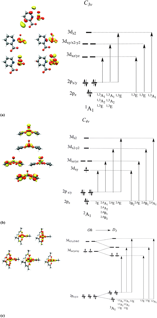
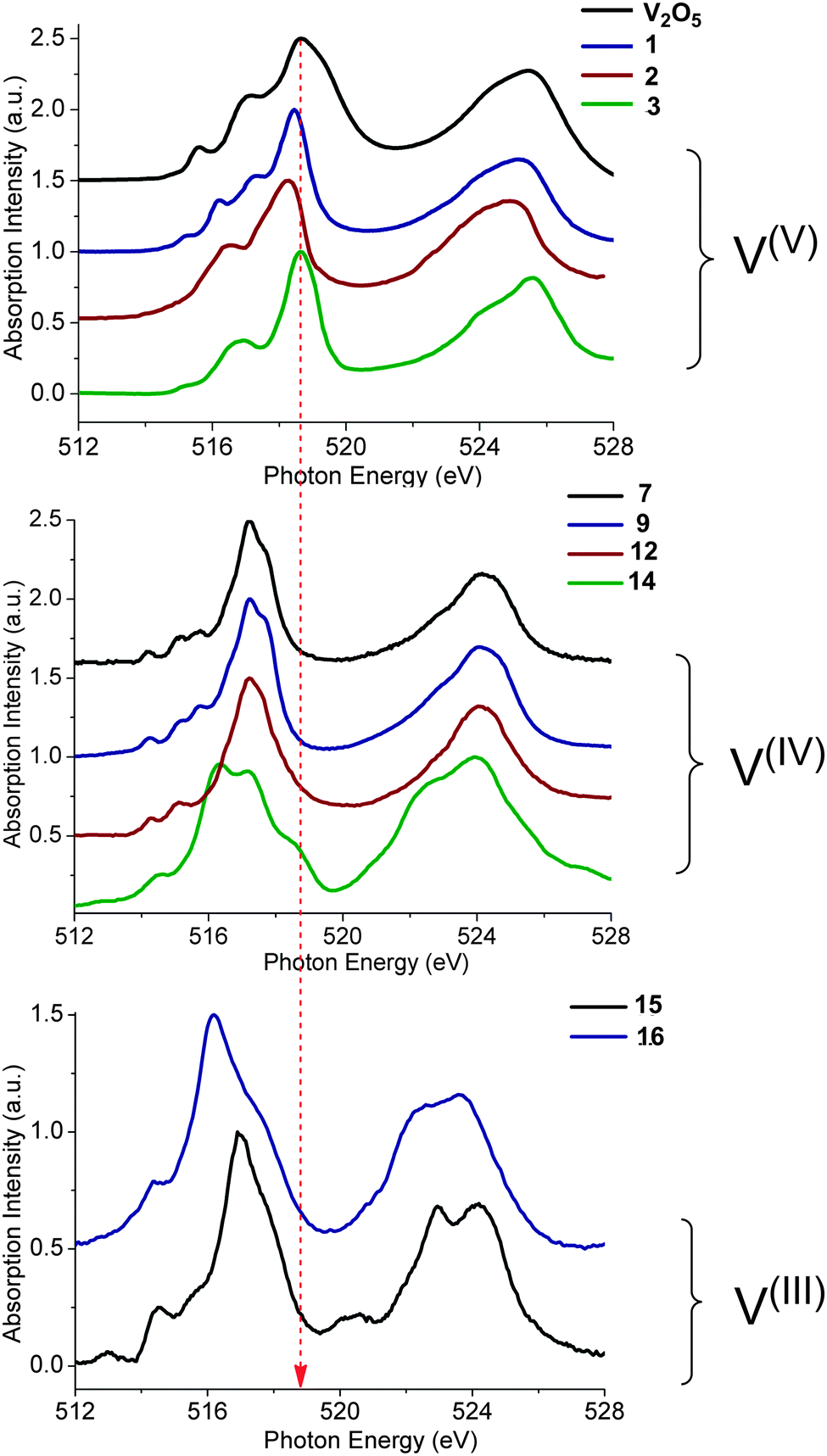
The V L-edge absorption data were obtained for the series of mononuclear vanadium complexes and treated following the procedures described in the Experimental section. As described above, the V L-edge spectra consist of two main signals belonging to the low-energy L3 and the high-energy L2 spectral regions. Among these regions, the L3 feature carries the largest amount of information as it further splits due to the ligand field splitting around the vanadium centers. On the other hand, in the L2 region, the corresponding information is usually obscured, due to the presence of Coster–Kronig Auger decay channels.74 Hence, in most cases one unresolved broad signal is observed at the L2-edge.
Further information can be obtained if the experimental spectra are grouped according to the formal oxidation state of vanadium (Fig. 3). This analysis, although still qualitative in nature, helps to further organize the experimental data. The most important observation from such spectral ordering is the shift of all discernible spectral features to lower energies upon reduction of the vanadium center along the sequence V(V) → V(IV) → V(III). This is consistent with expectation based on the effective nuclear charge of the metal center and the XAS edge energy. Such shifts amount to approximately 1 eV between the formal oxidation states of V(V) and V(IV). The respective V L-edge signals for the V(III)complexes are further shifted by approximately 0.5 eV to lower energy. Furthermore, for the six-coordinate V(V)-complexes 3–6 the L3 edge signal is primarily dominated by two or three features ordered in increasing energy. Additional features, however, occur in the case of V(V)-complexes in an approximate trigonal bipyramidal coordination environment, e.g. complexes 1 and 2. Furthermore, the corresponding L3 spectral region of V(IV) complexes 7–12, in a square pyramidal ligand field environment, shows a characteristic low energy pattern in the 514–517 eV spectral region. In addition, much broader features are observed in the case of complex 14 in which vanadium is coordinated in a tetrahedral environment. Likewise, the V(III) L-edge spectra (complexes 15, 16) are also characteristic, containing a ‘fingertip’ feature located at the low energy side of L3 (at ∼515 eV) and/or between the L3 and L2 regions (at ∼520 eV). Not surprisingly, the V(III) L3 spectra are much less resolved compared with the V(IV) and V(V) ones as a result of the large number of contributing states as discussed above and are more thoroughly analyzed below.
 |
| | Fig. 3 Experimental L-edge spectra of a selection of vanadium complexes grouped in different oxidation states: (a) V(V), (b) V(IV) and (c) V(III). The red dashed line indicates the shift of the spectra with respect to the energy position of the V2O5 reference L3 main spectral feature. A complete list of experimental spectra can be found in the ESI† (Fig. S1–S16). | |
Quantitative analysis.
It is desirable to translate the spectroscopic observables into electronic structure information. The most accepted procedure involves fitting of the observed spectra, followed by correlation of the fitted parameters with the structural and electronic properties. Such an approach has been successfully applied in the field of metal and ligand K-edge spectra.19,20,44–46 In fact, data analysis has shown that the absolute normalized intensities correlate with the type of the metal centers and ligand field environments, as well as the oxidation and spin states for a variety of studied systems. In addition, most of these correlations have been confirmed by electronic structure calculations. On the other hand, in the field of metal L-edge spectra similar approaches are not applicable without limitations. For the V L-edges a proper fitting procedure involves background-subtraction approaches to account for the overlapping L3 and L2, as well as O K-edge spectral features. Hence, it is anything but trivial to obtain quantitative results with respect to the absolute normalized intensities of the L3 and L2 features, the relative L3![[thin space (1/6-em)]](https://www.rsc.org/images/entities/char_2009.gif) :L2 area and the energetic separation between the L3- and L2-features.75,76 In fact, as has been discussed recently for metal L-edges the only experimental observables with a small degree of error refer to the overall L-edge spectral shape and the distribution of the observed features in the L3-region.42 Hence, the usual fitting procedure based on the total number of the observed features is not the method of choice here, as it cannot be correlated with any approach that ensures an unambiguous estimation of the origin, the number and the relative intensities, of the dominating transition probabilities. A qualitative approach to model these properties proceeds through Ligand Field Theory (LFT) approaches. The main aspects of these approaches have been explored in the semiempirical ligand field multiplet (LFM) and charge transfer multiplet (CTM) methods.16,30–32,39–41 However, as these methods are highly parameterized they are best used as tools to simulate experimental spectra and investigate trends among series of similar systems. On the other hand, a quantitative estimation of the number or the origin of the dominant states corresponding to the observed spectra in a predictive fashion requires more rigorous ab initio approaches, like the DFT/ROCIS method.
:L2 area and the energetic separation between the L3- and L2-features.75,76 In fact, as has been discussed recently for metal L-edges the only experimental observables with a small degree of error refer to the overall L-edge spectral shape and the distribution of the observed features in the L3-region.42 Hence, the usual fitting procedure based on the total number of the observed features is not the method of choice here, as it cannot be correlated with any approach that ensures an unambiguous estimation of the origin, the number and the relative intensities, of the dominating transition probabilities. A qualitative approach to model these properties proceeds through Ligand Field Theory (LFT) approaches. The main aspects of these approaches have been explored in the semiempirical ligand field multiplet (LFM) and charge transfer multiplet (CTM) methods.16,30–32,39–41 However, as these methods are highly parameterized they are best used as tools to simulate experimental spectra and investigate trends among series of similar systems. On the other hand, a quantitative estimation of the number or the origin of the dominant states corresponding to the observed spectra in a predictive fashion requires more rigorous ab initio approaches, like the DFT/ROCIS method.
Calibration.
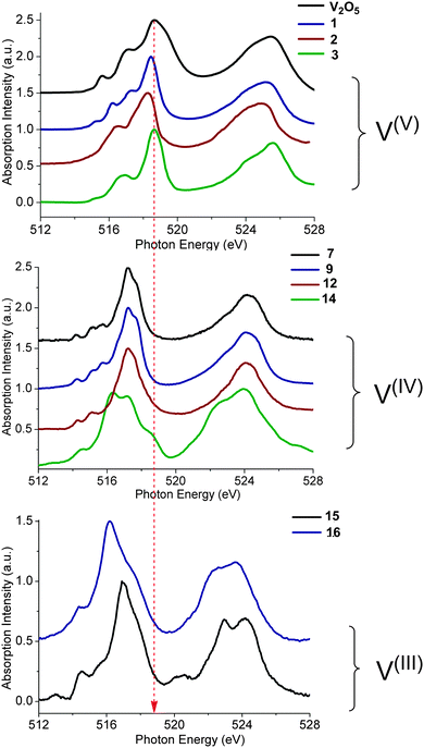
Prior to the calculation of the spectra a calibration was performed. As discussed above, owing to the limitations of DFT to accurately estimate the energies of the transition probabilities dominating the V L-edge spectra an empirical, element specific, shift should be determined. The calibration protocol followed here refers to a well-established methodological quantitative comparison between experimental and calculated core electron excited spectra.19,20,44–46 Its general aspects have been successfully applied to metal K-edges and an accordingly modified version of it will be presented in this section for the case of V L-edges. The most important result of this calibration is the determination of the energy shift for the calculation of V L-edge spectra (V-shift). After considerable experimentation with various alternative schemes, we have chosen to exclude the L2 part of the metal L-edges from the parameterization procedure as this feature is subject to extra broadening and distortion due to the Coster–Kronig Auger decay process74 which cannot be estimated accurately from experiment and is not treated at all within the DFT/ROCIS framework. The spectra were shifted to ensure that the highest intensity feature of the experimental and calculated L3 spectra is located at the same energy position. In practice, the energy position of the L3 calculated intensity maximum  is shifted to match the corresponding experimental one. The V-shift value is then extracted by averaging over all individual shifts in the course of a linear least-square correlation of the experimental and the calculated spectra (Fig. 4).
 |
| | Fig. 4 Relationship of calculated versus experimentally determined transition energies for B3LYP/def2-SVP (upper left), B3LYP/def2-TZVP(-f) (upper right), BHLYP/def2-SVP (lower left) and BHLYP/def2-TZVP(-f) (lower right). The linear least-squares fits are given by fB3LYP/def2–SVP = 1.50(exp) − 275.54 eV, fB3LYP/def2–TZVP(-f) = 1.40(exp) − 224.22 eV, fBHLYP/def2–SVP = 1.77(exp) − 397.54 eV and fBHLYP/def2-TZVP = 1.63(exp) − 326.91. The notation exp refers to experimental values in eV. | |
Effect of functional and basis sets.
In this section the effect of the chosen functional and basis set combinations on the V-shift is investigated. Two density functionals, namely B3LYP and BHLYP, as well as two basis sets, def2-SVP and def2-TZVP(-f), respectively, were used to scale the c parameters of the DFT/ROCIS method.42 Thus, the V-shift is discussed for four functional-basis set combinations. As can be seen in Fig. 4 and Table 1, in all the cases an acceptable linear correlation between calculated and experimental energies is observed. From each of these relations, the element shift, V-shift: ΔEV, can be extracted. For the B3LYP functional this shift is positive, amounting to  and to
  for def2-SVP and def2 TZVP basis sets, respectively. On the other hand, for BHLYP the shift is negative, corresponding to
 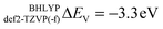 and
and  for the def2-SVP and def2-TZVP(-f) basis sets respectively. In general, slightly better linear relations are observed with a triple-zeta quality basis set, which also provide somewhat narrower error distribution as can be seen in Fig. 4. Nevertheless, the overall shape of all the calculated versus experimental spectra, independent of the chosen functional and basis set combination, is generally good to very good as can be seen in Fig. 5a–c and Fig. S1–S16, (ESI†). It should be noted that the main deviations between theory and experiment are found to be around the L2 region of the spectra. This is not surprising, as this region is also not unambiguously determined by either experiment. As expected, these deviations become more pronounced as more and more final states come into play. This is the case upon going from VV to VIII. Another point refers to the linear correlation of the experimental versus calculated transition energy
  for the VIV systems in the test set. Owing to the broadening of the experimental spectra, the observed linear distribution is worse compared with the complexes for the other oxidation states. However, generally speaking, there is an excellent linear relationship between calculated and measured excitations energies, which indicates that the DFT/ROCIS method is applicable to diverse and large systems. A notable loss of accuracy upon moving to smaller basis sets is not expected but will lead to significantly shorter calculation times, in particular for large polymetallic systems. These expectations have recently been successfully tested for V2O5, in which cluster models up to 20 vanadium centers were treated.43
Table 1 Calculated versus experimental L3 maximum energy positions  for all the complexes of the training set (1–16) as well as the corresponding V-shift: ΔEV for all the functional and basis set combinations, namely B3LYP/def2-SVP, B3LYP/def2-TZVP(-f), BHLYP/def2-TZVP(-f) and BHLYP/def2-SVP
| Complexes |
Num |

|

|
| B3LYP/def2-SVP |
B3LYP/def2-TZVP(-f) |
BHLYP/def2-SVP |
BHLYP/def2-TZVP(-f) |
|
V(V)
|
| [VO(O2)2C5H4NCOO]2 |
1
|
518.5 |
506.9 |
505.5 |
523.0 |
521.5 |
| [VO(O2)2C2O4]2 |
2
|
518.6 |
506.8 |
505.5 |
523.0 |
521.6 |
|
|
| [V(O)2H,MeL3] |
3
|
518.5 |
506.3 |
505.3 |
522.1 |
520.8 |
| [V(O)2H,PhL3] |
4
|
518.2 |
505.9 |
505.1 |
521.7 |
520.7 |
| [V(O)2H,PhNO2L3] |
5
|
518.3 |
505.9 |
505.2 |
521.7 |
520.6 |
| [V(O)2Me,PhL3] |
6
|
518.4 |
506.3 |
505.3 |
522.1 |
520.8 |
|
|
|
V(IV)
|
| [V(O)(acac)2] |
7
|
517.2 |
505.1 |
504.1 |
520.9 |
519.7 |
| [V(O)(acac)2(Py)] |
8
|
517.2 |
505.0 |
504.1 |
521.1 |
519.4 |
| [V(O)(TPP)] |
9
|
517.3 |
504.6 |
503.7 |
519.9 |
518.9 |
| [V(O)(HMeL2)(O)] |
10
|
517.2 |
504.9 |
504.0 |
520.4 |
519.3 |
| [V(O)(HEtL2)(O)] |
11
|
517.3 |
504.8 |
504.0 |
520.3 |
519.1 |
| [V(O)(HClL2)(O)] |
12
|
517.2 |
504.9 |
504.1 |
520.5 |
519.4 |
| [V(O)(salen)] |
13
|
517.2 |
504.3 |
503.4 |
520.1 |
518.9 |
| [V(MeO)L3] |
14
|
517.2 |
505.0 |
504.0 |
520.3 |
519.7 |
|
|
|
V(III)
|
| [V(acac)3] |
15
|
516.9 |
504.6 |
503.4 |
519.2 |
518.0 |
| [V(MeOH)L3] |
16
|
516.2 |
502.2 |
501.4 |
517.9 |
517.0 |
|
|
|
V-shift (ΔEV, eV) |
|
|
12.3
|
13.3
|
−2.1
|
−3.3
|
 |
| | Fig. 5 Experimental versus calculated DFT/ROCIS def2-TZVP(-f) spectra of the complexes (a) 1, (b) 7 and (c) 15. The corresponding spectra for B3LYP (left) and BHLYP (right) functionals are visualized. | |
Nature of core to valence features
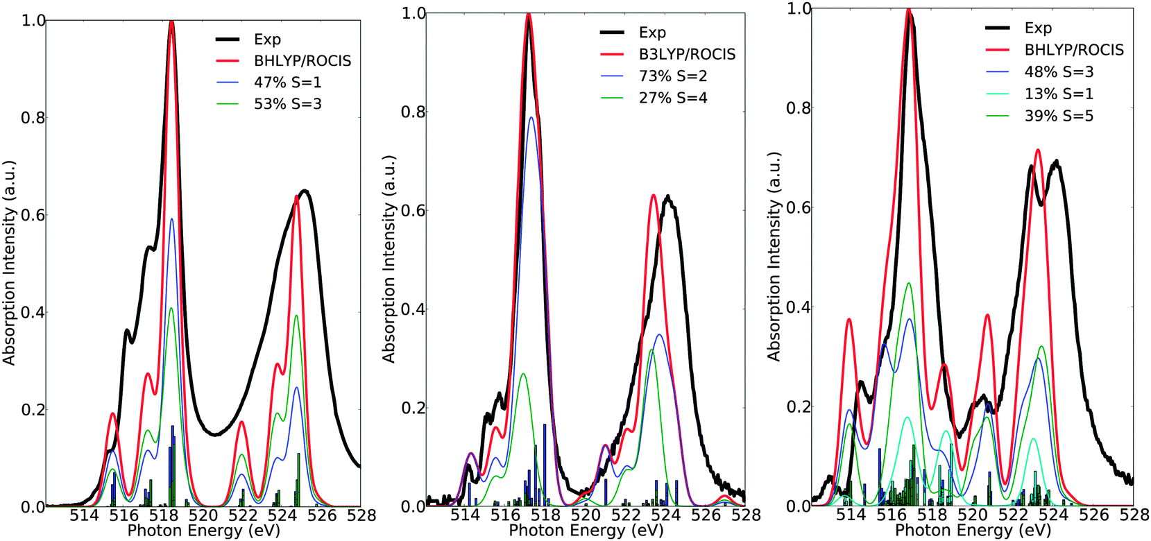
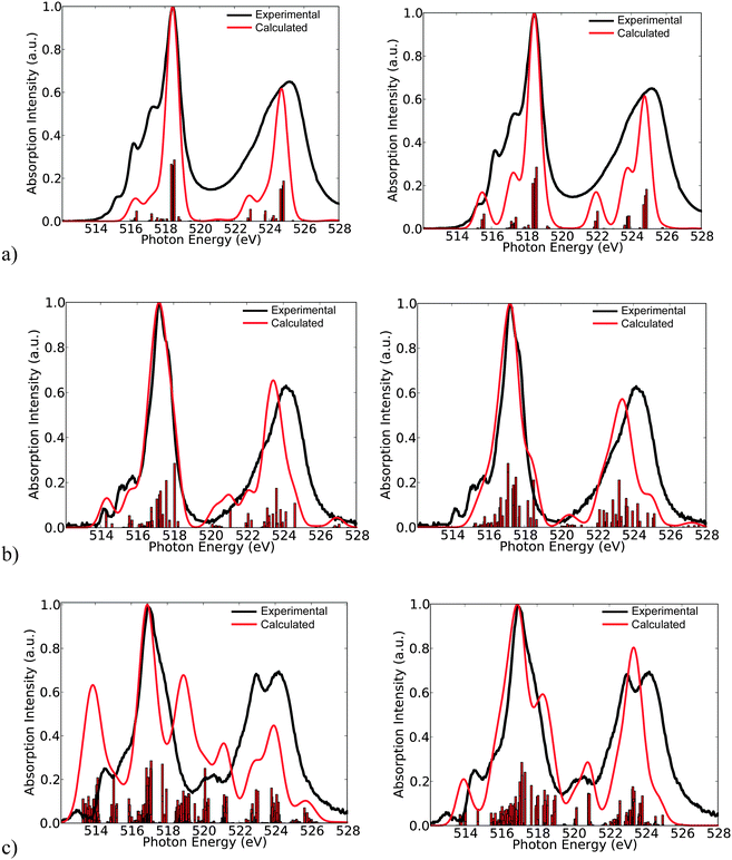
Here, the intensity distribution of the vanadium L-edge spectra is further discussed. As can be seen in Fig. 5 and Fig. S1–S16 (ESI†) the calculated spectra of the test set of complexes 1–16 are dominated by a large number of states, which reflect the local electronic structure of the vanadium centers. It is thus desirable to extend the analysis and characterize these states in terms of their spin multiplicities S = 2S + 1, their magnetic quantum numbers Ms, as well as their dominant single electron 2p → 3d excitation characters. This is possible, as in most of the cases the calculated many particle states are characterized by small or moderately small multiconfigurational character. As can be seen in Fig. 6 the spectra of complexes 1, 7 and 15 are dominated by the corresponding ground state multiplicities. In addition they contain significant contributions from states with higher (1, 7 and 15) or lower spin multiplicities (15). In particular, for the d0 complex 1, the contribution of the triplet increases to 53%, which is expected, since for a closed shell d0 complex there is an equal probability of generating a core to the valence excited singlet or the triplet state. On the other hand for the case of the d1 complex 7, the contribution of the quartet states amounts to only 27%, and thus the spectrum is dominated mainly by the doublet states (73%). The situation gets significantly more complicated for the d2 complex 15, in which contributions from states of lower multiplicities come into play. Hence, only half of the calculated intensity derives from triplet states (48%) while the remaining half contains contributions from the excited quintet (39%) and singlet (13%) states, respectively.
 |
| | Fig. 6 Calculated (red) versus experimental spectra (black) of complexes 1 (left), 7 (middle) and 15 (right). Blue, green and cyan lines represent deconvolution of the calculated spectrum in terms of dominant states with spin multiplicity S. | |
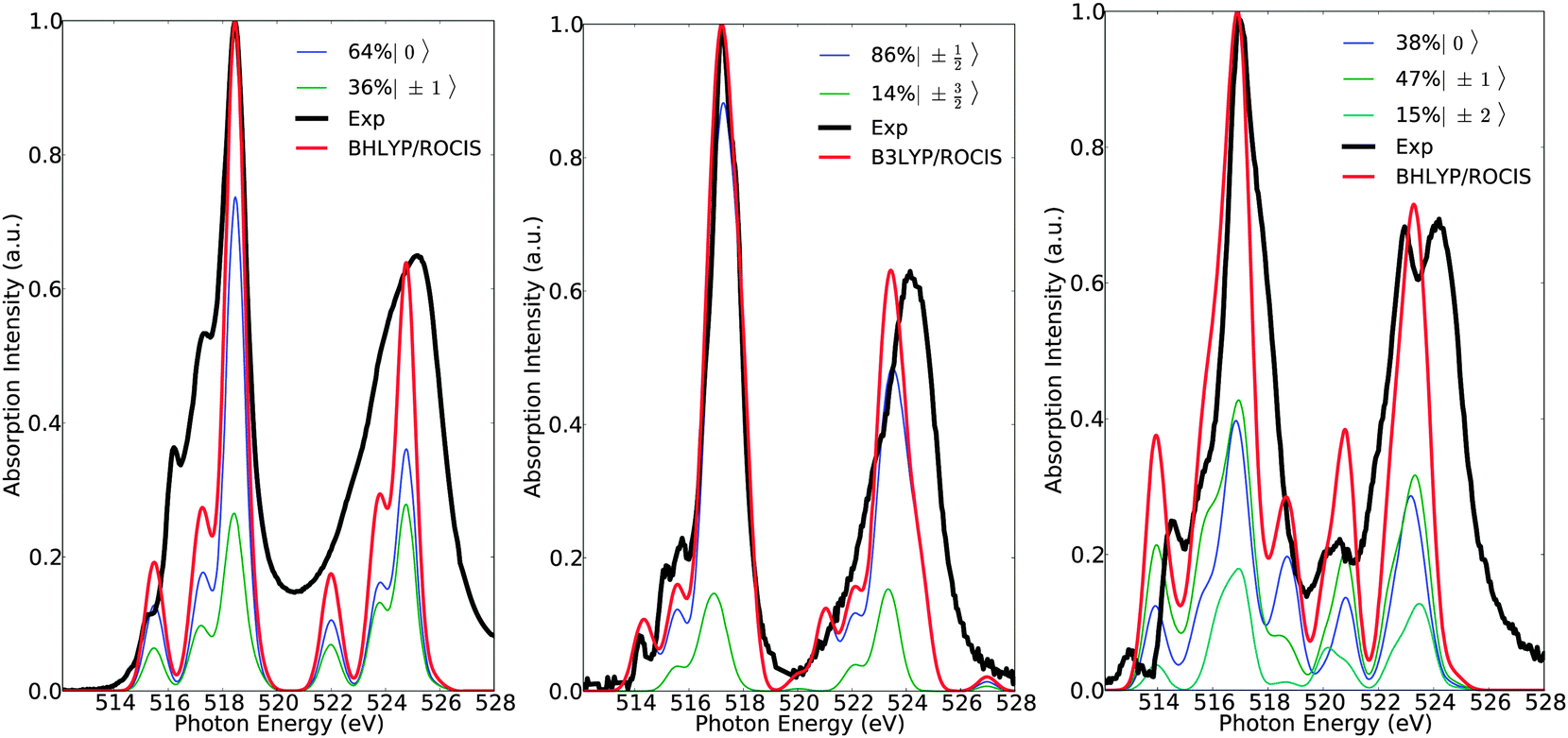
Of course, any state of multiplicity S is mixed through quasi-degenerate perturbation theory (QDPT) and any remaining spin degeneracy prior to SOC treatment is altered. Thus, it is more appropriate to refer to the contributing final states with their Ms component, rather than by their spin multiplicity prior to SOC treatment. This is reasonable as the total spin is a good quantum number in each of these states. Therefore, in a further step of analysis, the calculated spectra can be deconvoluted in terms of the dominant magnetic sublevels (Fig. 7). As can be seen in Fig. 7, the calculated spectra of complexes 1, 7 and 15 are dominated by the ground magnetic sublevels 64%〉|0〉, 85%|±½〉 and 45%〉|±1〉, respectively, containing, in addition, contributions from the corresponding relevant magnetic sublevels of the following characters: 36%|±1〉, 14%|±〉 and 15%|±2〉 + 38%|0〉.
 |
| | Fig. 7 Calculated (red) versus experimental spectra (black) of complexes 1 (left), 7 (middle) and 15 (right). Blue, green and cyan lines represent deconvolution of the calculated spectra in terms of dominant states with magnetic quantum number Ms. | |
Further deconvolution in terms of dominant 2p → 3d excitations is straightforward as can be seen in Fig. 8. Without investing extra effort, by combining the above information, it is possible to achieve a comprehensive analysis of the L3 spectra. For complex 1, analysis of the individual excitations indicates a distorted, trigonally symmetric, geometry around the vanadium center, which is consistent with the idealized C3v symmetric ligand field picture given in Fig. 3. The lower energy feature at 515 eV is dominated by the states 60%|0〉 + 40%|±1〉 involving the 2p → 3dyz single electron excitations. The next two features at 516 eV and 517 eV are dominated by overlapping states of 75%|0〉 + 25%|±1〉 character, involving the 2p → 3dxy and 2p → 3dxz excitations. Finally, the highest energy feature at 518.5 eV corresponds to states of 85%|0〉 + 15%|±1〉 character dominated by the 2p → 3dx2−y2 and 2p → 3dz2 excitations. Analogously, for complex 7 the overall excitation pattern is in close resemblance with the LFT picture of vanadium in a distorted tetragonal coordination environment. The signal at 514 eV is dominated solely by the doublet states |±½〉 which involve the DOMO → SOMO 2p → 3dxy excitations. The signals at 515.1 and 515.6 eV are dominated by a combination of states 66%|±½〉 + 33%|±〉 of excitation character 2p → 3dxz. On the other hand, the main line at 517.1 eV is dominated by a group of states of 87%|±½〉 + 13%|±〉 character, containing contributions from the 2p → 3dyz, 3dx2−y2, 3dz2 one-electron excitations respectively. The situation is even more complicated for complex 15, in which the main spectral features are dominated by a large number of states (Fig. 5 and 6). As a result, a clear departure from the simple LFT picture occurs, as shown in Fig. 3. In particular, the low energy feature at 514.5 eV corresponds to 50%|±1〉 + 30%|±2〉 + 10%|0〉 states, which are dominated by 2p → 3dxy, 3dyz excitations, whereas the main line, as well as the signals located at 516, 515.5 and 517.8 eV respectively, are composed from states with 42%|±1〉 + 40%|±2〉 + 18%|0〉 character, involving the 2p → 3dyz, 3dx2−y2, 3dz2 excitations.
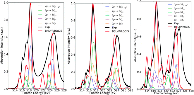 |
| | Fig. 8 Calculated (red) versus experimental spectra (black) of complexes 1 (left), 7 (middle) and 15 (right). Blue, green, cyan, purple and orange lines represent deconvolution of the calculated spectrum in terms of dominating 2p → 3d single electron excitations. | |
Conclusion
In this work we present a systematic experimental and computational study on V L-edge XAS spectra of a series of mononuclear vanadium complexes. All complexes 1–16 exhibit excellent quality spectra with well-resolved L3 features. The shape, as well as the energy position of the spectra, proved to be sensitive to the chemical environment surrounding the vanadium centers (e.g. the vanadium oxidation and spin states as well as the ligand identity and geometry).
In addition to the experimental investigations the recently developed DFT/ROCIS method was applied to calculate and interpret the experimentally observed V L-edge spectra. Upon treating the multiplet structure of the many particle final states with proper Configuration Interaction techniques, as well as dynamic correlation effects in the framework of DFT, and accounting for SOC with QDPT very good to excellent results were obtained.
The systematic and element specific energy shift between experimental and theoretical spectra was determined for all the combinations of B3LYP and BHLYP functionals with the def2-SVP and def2-TZVP(-f) basis sets. Results of the similarly good quality were obtained for all functional and basis-set combinations indicating stability and transferability of the method to larger systems.
Furthermore a detailed investigation of the nature of the observed experimental features was performed for complexes 1, 7 and 15 in oxidation states V(V), V(IV) and V(III) respectively. The results were analyzed in terms of dominant magnetic sublevels in variable spin multiplicities and magnetic quantum numbers. These results were further mapped into a Ligand Field picture providing the contributions from the dominant single electron 2p to 3d excitations. Such flexibility allows for a direct connection between the experimentally probed states with the molecular orbital theory, and thus to function in chemical reaction. The observed spectral features are found to be sensitive to both the chemical environment surrounding the vanadium center (number of ligands, ligand identity, coordination geometry) as well as its oxidation and spin state. Furthermore, the analysis of the experimental features in terms of contributing magnetic sublevels is the most accessible scheme. On the other hand a simplified Ligand Field picture proved to be the least preferable choice to describe the observed spectral features, as it essentially breaks down with the increasing number of the involved final states (or with a decrease in the vanadium oxidation states). Future work will focus on more targeted electronic structure questions that can be addressed by metal L-edge spectroscopy. An example is given in the ESI† regarding correlations between ligand field strength and metal oxidation states (Fig. S17, ESI†).
In conclusion, the observed strong influence on the spectral shape of the vanadium oxidation and spin states, as well as the ligand environment, in combination with the strong correlation between theory and experiment, provides a strongly predictive and quantitative tool for examining catalytic intermediates of vanadium compounds.
Acknowledgements
FN, SD and RS gratefully acknowledge financial support of this work by the Max Planck Society. The Helmholtz-Zentrum Berlin (HZB) staff is acknowledged for continuously supporting the synchrotron based near ambient pressure spectroscopy experiments of the Fritz Haber Institute at BESSY II. Professor Nigel Young is kindly acknowledged for providing raw data of complexes 2–6, 8 and 11–15. The reviewers of the manuscript are thanked for their constructive comments.
References
- B. M. Weckhuysen and D. E. Keller, Catal. Today, 2003, 78, 25 CrossRef CAS.
- J. L. Nieto, Top. Catal., 2006, 41, 3 CrossRef PubMed.
- B. Grzybowska-Świerkosz, Appl. Catal., A, 1997, 157, 263 CrossRef.
- P. Forzatti, Appl. Catal., A, 2001, 222, 221 CrossRef CAS.
- E. A. Mamedov and V. Cortés Corberán, Appl. Catal., A, 1995, 127, 1 CrossRef CAS.
- P. Gruene, T. Wolfram, K. Pelzer, R. Schlögl and A. Trunschke, Catal. Today, 2010, 157, 137 CrossRef CAS PubMed.
- J. E. Molinari and I. E. Wachs, J. Am. Chem. Soc., 2010, 132, 12559 CrossRef CAS PubMed.
- C. Hess, ChemPhysChem, 2009, 10, 319 CrossRef CAS PubMed.
- I. Muylaert and P. Van Der Voort, Phys. Chem. Chem. Phys., 2009, 11, 2826 RSC.
- A. Khodakov, B. Olthof, A. T. Bell and E. Iglesia, J. Catal., 1999, 181, 205 CrossRef CAS.
- M. Cavalleri, K. Hermann, A. Knop-Gericke, M. Hävecker, R. Herbert, C. Hess, A. Oestereich, J. Döbler and R. Schlögl, J. Catal., 2009, 262, 215 CrossRef CAS PubMed.
- M. Hävecker, M. Cavalleri, R. Herbert, R. Follath, A. Knop-Gericke, C. Hess, K. Hermann and R. Schlögl, Phys. Status Solidi B, 2009, 246, 1459 CrossRef.
- M. Hävecker, A. Knop-Gericke, H. Bluhm, E. Kleimenov, R. W. Mayer, M. Fait and R. Schlögl, Appl. Surf. Sci., 2004, 230, 272 CrossRef PubMed.
- M. Hävecker, N. Pinna, K. Weiß, H. Sack-Kongehl, R. E. Jentoft, D. Wang, M. Swoboda, U. Wild, M. Niederberger, J. Urban, D. S. Su and R. Schlögl, J. Catal., 2005, 236, 221 CrossRef PubMed.
- E. Kleimenov, H. Bluhm, M. Hävecker, A. Knop-Gericke, A. Pestryakov, D. Teschner, J. A. Lopez-Sanchez, J. K. Bartley, G. J. Hutchings and R. Schlögl, Surf. Sci., 2005, 575, 181 CrossRef CAS PubMed.
-
F. M. F. de Groot and A. Kotani, Core Level Spectroscopy of Solids, CRC Press, 2008 Search PubMed.
- J. G. Chen, Surf. Sci. Rep., 1997, 30, 1 CrossRef CAS.
- A. I. Nesvizhskii and J. J. Rehr, J. Synchrotron Radiat., 1999, 6, 315 CrossRef CAS PubMed.
- S. DeBeer George and F. Neese, Inorg. Chem., 2010, 49, 1849 CrossRef CAS PubMed.
- S. DeBeer George, T. Petrenko and F. Neese, Inorg. Chim. Acta, 2008, 361, 965 CrossRef CAS PubMed.
- S. DeBeer George, T. Petrenko and F. Neese, J. Phys. Chem. A, 2009, 112, 12936 CrossRef PubMed.
- C. Kolczewski and K. Hermann, J. Chem. Phys., 2003, 118, 7599 CrossRef CAS.
- C. Kolczewski and K. Hermann, Surf. Sci., 2004, 552, 98 CrossRef CAS PubMed.
- C. Kolczewski and K. Hermann, Phys. Scr., T, 2005, 115, 128 CrossRef.
- M. Cavalleri, H. Ogasawara, L. G. M. Pettersson and A. Nilsson, Chem. Phys. Lett., 2002, 364, 363 CrossRef CAS.
- M. G. Brik, K. Ogasawara, H. Ikeno and I. Tanaka, Eur. Phys. J. B, 2006, 51, 345 CrossRef CAS.
- P. Krueger and C. R. Natoli, Phys. Rev. B: Condens. Matter Mater. Phys., 2004, 70, 245120 CrossRef.
- C. R. Natoli, M. Benfatto, C. Brouder, M. F. Lopez and D. L. Foulis, Phys. Rev. B: Condens. Matter Mater. Phys., 1990, 42, 1944 CrossRef.
- A. L. Ankudinov, A. I. Nesvizhskii and J. J. Rehr, Phys. Rev. B: Condens. Matter Mater. Phys., 2003, 67, 115120 CrossRef.
- F. M. F. de Groot, Coord. Chem. Rev., 2005, 249, 31 CrossRef CAS PubMed.
- F. M. F. de Groot, J. Electron Spectrosc. Relat. Phenom., 1994, 67, 529 CrossRef CAS.
- A. Kotani, J. Electron Spectrosc. Relat. Phenom., 1999, 100, 75 CrossRef CAS.
- H. Ikeno, T. Mizoguchi and I. Tanaka, Phys. Rev. B: Condens. Matter Mater. Phys., 2011, 83, 155107 CrossRef.
- H. Ikeno, I. Tanaka, Y. Koyama, T. Mizoguchi and K. Ogasawara, Phys. Rev. B: Condens. Matter Mater. Phys., 2005, 72, 075123 CrossRef.
- Y. Kumagai, H. Ikeno, F. Oba, K. Matsunaga and I. Tanaka, Phys. Rev. B: Condens. Matter Mater. Phys., 2008, 77, 155124 CrossRef.
- K. Ogasawara, T. Iwata, Y. Koyama, T. Ishii, I. Tanaka and H. Adachi, Phys. Rev. B: Condens. Matter Mater. Phys., 2001, 64, 115413 CrossRef.
- P. S. Bagus, H. Freund, H. Kuhlenbeck and E. S. Ilton, Chem. Phys. Lett., 2008, 455, 331 CrossRef CAS PubMed.
-
M. Haverkort, M. Zwierzycki and O. Andersen, arxiv preprint arXiv:1111.4940, 2011.
- B. T. Thole and G. van der Laan, Phys. Rev. A: At., Mol., Opt. Phys., 1988, 38, 1943 CrossRef CAS.
- B. T. Thole and G. van der Laan, Phys. Rev. B: Condens. Matter Mater. Phys., 1988, 38, 3158 CrossRef CAS.
- G. van der Laan, B. T. Thole, G. A. Sawatzky and M. Verdaguer, Phys. Rev. B: Condens. Matter Mater. Phys., 1988, 37, 6587 CrossRef CAS.
- M. Roemelt, D. Maganas, S. DeBeer and F. Neese, J. Chem. Phys., 2013, 138, 204101 CrossRef PubMed.
- D. Maganas, M. Roemelt, M. Havecker, A. Trunschke, A. Knop-Gericke, R. Schlogl and F. Neese, Phys. Chem. Chem. Phys., 2013, 15, 7260 RSC.
- N. Lee, T. Petrenko, U. Bergmann, F. Neese and S. DeBeer, J. Am. Chem. Soc., 2010, 132, 9715 CrossRef CAS PubMed.
- M. A. Beckwith, M. Roemelt, M.-N. l. Collomb, C. DuBoc, T.-C. Weng, U. Bergmann, P. Glatzel, F. Neese and S. DeBeer, Inorg. Chem., 2011, 50, 8397 CrossRef CAS PubMed.
- M. Roemelt, M. A. Beckwith, C. Duboc, M.-N. Collomb, F. Neese and S. DeBeer, Inorg. Chem., 2011, 51, 680 CrossRef PubMed.
- D. Collison, C. David Garner, J. Grigg, C. M. McGrath, J. F. W. Mosselmans, E. Pidcock, M. D. Roper, J. M. W. Seddon, E. Sinn, P. A. Tasker, G. Thornton, J. F. Walsh and N. A. Young, J. Chem. Soc., Dalton Trans., 1998, 2199 RSC.
- T. Kajiwara, R. Wagner, E. Bill, T. Weyhermuller and P. Chaudhuri, Dalton Trans., 2011, 40, 12719 RSC.
- A. Shaver, J. B. Ng, D. A. Hall, B. S. Lum and B. I. Posner, Inorg. Chem., 1993, 32, 3109 CrossRef CAS.
- P. Banerjee, S. Sproules, T. Weyhermüller, S. DeBeer George and K. Wieghardt, Inorg. Chem., 2009, 48, 5829 CrossRef CAS PubMed.
- M. Roemelt and F. Neese, J. Phys. Chem. A, 2013, 117, 3069 CrossRef CAS PubMed.
- F. Neese, J. Am. Chem. Soc., 2006, 128, 10213 CrossRef CAS PubMed.
- B. A. Hess, C. M. Marian, U. Wahlgren and O. Gropen, Chem. Phys. Lett., 1996, 251, 365 CrossRef CAS.
- C. M. Marian and U. Wahlgren, Chem. Phys. Lett., 1996, 251, 357 CrossRef CAS.
- F. Neese, J. Chem. Phys., 2005, 122, 34107 CrossRef PubMed.
- F. Neese, T. Petrenko, D. Ganyushin and G. Olbrich, Coord. Chem. Rev., 2007, 251, 288 CrossRef CAS PubMed.
-
F. Neese, W. Ames, G. Christian, M. Kampa, D. G. Liakos, D. A. Pantazis, M. Roemelt, P. Surawatanawong and Y. E. Shengfa, in Advances in Inorganic Chemistry, ed. E. Rudi van and H. Jeremy, Academic Press, 2010, vol. 62, p. 301 Search PubMed.
- B. A. Hess, Phys. Rev. A: At., Mol., Opt. Phys., 1985, 32, 756 CrossRef CAS.
- B. A. Hess, Phys. Rev. A: At., Mol., Opt. Phys., 1986, 333, 3742 CrossRef.
- G. Jansen and B. A. Hess, Phys. Rev. A: At., Mol., Opt. Phys., 1989, 39, 6016 CrossRef.
- B. Sandhoefer and F. Neese, J. Chem. Phys., 2012, 137, 094102 CrossRef CAS PubMed.
- F. Neese, Wiley Interdiscip. Rev.: Comput. Mol. Sci., 2012, 2, 73 CrossRef CAS.
- A. D. Becke, Phys. Rev. A: At., Mol., Opt. Phys., 1988, 38, 3098 CrossRef CAS.
- J. P. Perdew, Phys. Rev. B: Condens. Matter Mater. Phys., 1986, 33, 8822 CrossRef.
- A. D. Becke, J. Chem. Phys., 1993, 98, 5648 CrossRef CAS.
- C. Lee, W. Yang and R. G. Parr, Phys. Rev. B: Condens. Matter Mater. Phys., 1988, 37, 785 CrossRef CAS.
- S. Grimme, J. Antony, S. Ehrlich and H. Krieg, J. Chem. Phys., 2010, 132, 154104 CrossRef PubMed.
- S. Grimme, S. Ehrlich and L. Goerigk, J. Comput. Chem., 2011, 32, 1456 CrossRef CAS PubMed.
- A. Schäfer, C. Huber and R. Ahlrichs, J. Chem. Phys., 1994, 100, 5829 CrossRef.
- M. Feyereisen, G. Fitzgerald and A. Komornicki, Chem. Phys. Lett., 1993, 208, 359 CrossRef CAS.
- R. A. Kendall and H. A. Früchtl, Theor. Chem. Acc., 1997, 97, 158 CrossRef CAS.
- D. A. Pantazis, X. Y. Chen, C. R. Landis and F. Neese, J. Chem. Theory Comput., 2008, 4, 908 CrossRef CAS.
- F. Neese, Coord. Chem. Rev., 2009, 253, 526 CrossRef CAS PubMed.
- D. Coster and R. D. L. Kronig, Physica, 1935, 2, 13 CrossRef CAS.
- L. J. Giles, A. Grigoropoulos and R. K. Szilagyi, J. Phys. Chem. A, 2012, 116, 12280–12298 CrossRef CAS PubMed.
- H. Tan, J. Verbeeck, A. Abakumov and G. Van Tendeloo, Ultramicroscopy, 2012, 116, 24 CrossRef CAS PubMed.
- F. Weigend and R. Ahlrichs, Phys. Chem. Chem. Phys., 2005, 7, 3297 RSC.
Footnote |
| † Electronic supplementary information (ESI) available. See DOI: 10.1039/c3cp52711e |
|
| This journal is © the Owner Societies 2014 |
Click here to see how this site uses Cookies. View our privacy policy here.  Open Access Article
 This Open Access Article is licensed under a
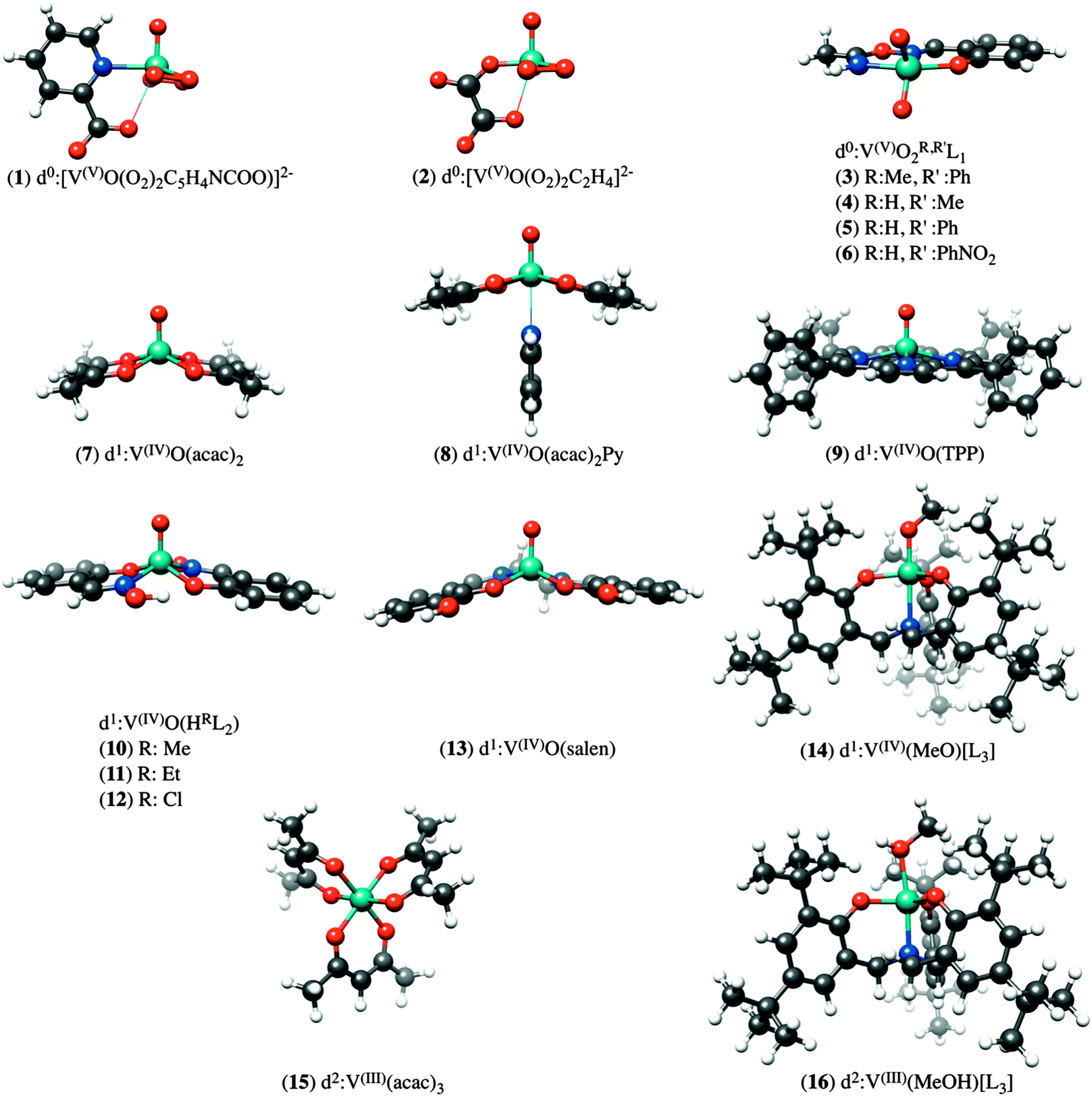

 denotes matrix elements of the exchange–correlation potential. Both matrices are given in the hybrid density functional form, since hybrid density functionals will be used in all presented DFT/ROCIS calculations. The coefficients cHF and cDF denote the amount of HF exchange and pure density functional related exchange–correlation contribution, respectively. Accordingly, for a HF calculation cDF = 0. The ROCIS method implicitly introduces dynamic electron correlation through three empirical parameters c1, c2 and c3. These parameters are used to scale the Coulomb and exchange integrals in the diagonal of the CI matrix, as well as the off-diagonal CI elements. For example, in the subspace spanned by the singly-excited configuration state functions (CSFs) arising from the single excitation from a DOMO i or j into a VMO a or b, the scaled CI matrix elements become:
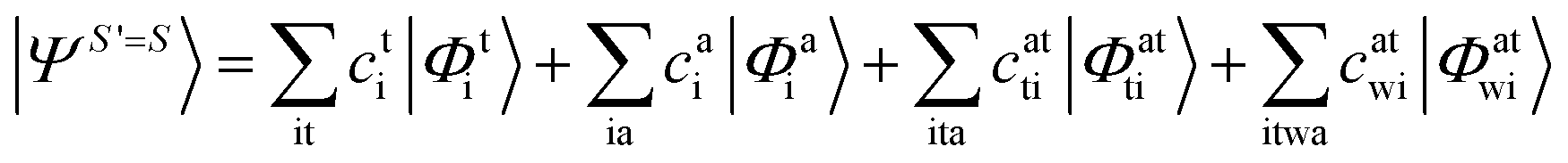
 . The upper indices SS denote a many-particle wavefunction with spin quantum number S and spin projection quantum number M = S. Since the BO Hamiltonian is spin free, only one member of a given spin-multiplet (e.g. that with M = S) needs to be calculated. For the treatment of the SOC all |ΨSMI〉 are required (I denotes a given state obtained in the first step of the procedure). Matrix elements over the |ΨSMI〉 functions are readily generated using the Wigner–Eckart theorem, since all (2S + 1) members of the multiplet share the same spatial part of the wavefunction:49
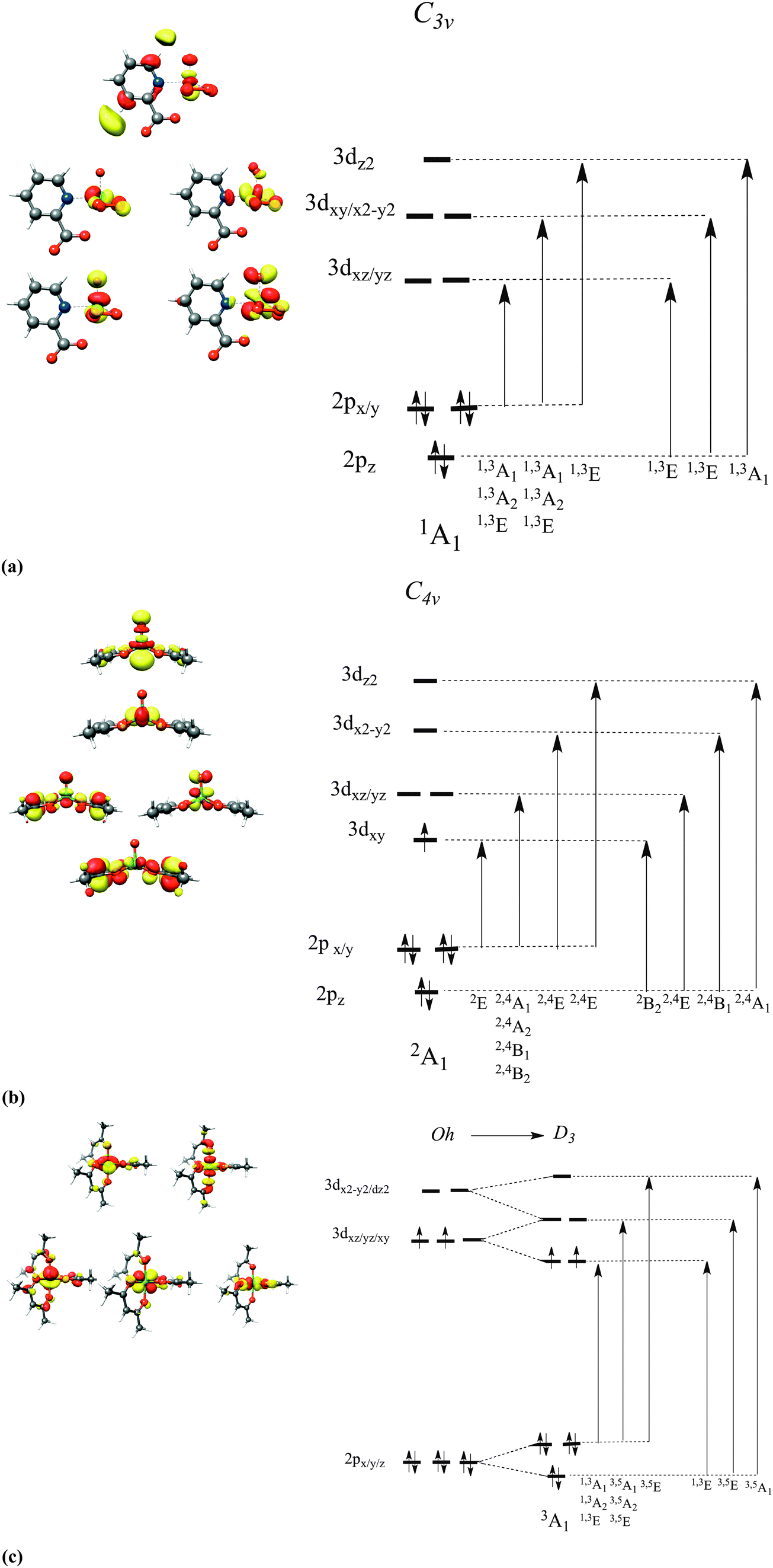
 is shifted to match the corresponding experimental one. The V-shift value is then extracted by averaging over all individual shifts in the course of a linear least-square correlation of the experimental and the calculated spectra (Fig. 4).

 and to
 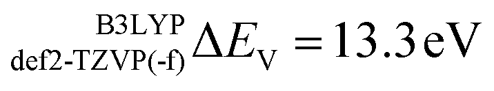 for def2-SVP and def2 TZVP basis sets, respectively. On the other hand, for BHLYP the shift is negative, corresponding to
 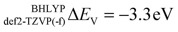 and
and  for the def2-SVP and def2-TZVP(-f) basis sets respectively. In general, slightly better linear relations are observed with a triple-zeta quality basis set, which also provide somewhat narrower error distribution as can be seen in Fig. 4. Nevertheless, the overall shape of all the calculated versus experimental spectra, independent of the chosen functional and basis set combination, is generally good to very good as can be seen in Fig. 5a–c and Fig. S1–S16, (ESI†). It should be noted that the main deviations between theory and experiment are found to be around the L2 region of the spectra. This is not surprising, as this region is also not unambiguously determined by either experiment. As expected, these deviations become more pronounced as more and more final states come into play. This is the case upon going from VV to VIII. Another point refers to the linear correlation of the experimental versus calculated transition energy
  for the VIV systems in the test set. Owing to the broadening of the experimental spectra, the observed linear distribution is worse compared with the complexes for the other oxidation states. However, generally speaking, there is an excellent linear relationship between calculated and measured excitations energies, which indicates that the DFT/ROCIS method is applicable to diverse and large systems. A notable loss of accuracy upon moving to smaller basis sets is not expected but will lead to significantly shorter calculation times, in particular for large polymetallic systems. These expectations have recently been successfully tested for V2O5, in which cluster models up to 20 vanadium centers were treated.43
 for all the complexes of the training set (1–16) as well as the corresponding V-shift: ΔEV for all the functional and basis set combinations, namely B3LYP/def2-SVP, B3LYP/def2-TZVP(-f), BHLYP/def2-TZVP(-f) and BHLYP/def2-SVP