 Open Access Article
 This Open Access Article is licensed under a
 Creative Commons Attribution 3.0 Unported Licence
Structural arrest and texture dynamics in suspensions of charged colloidal rods†
Kyongok
Kang
*a and
Jan K. G.
Dhont
ab
aForschungszentrum Jülich, Institute of Complex Systems (ICS), Soft Condensed Matter, D-52425 Jülich, Germany. E-mail: k.kang@fz-juelich.de; Web: http://www.fz-juelich.de/iff/d_iwm
bHeinrich-Heine-Universität Düsseldorf, Department of Physics, D-40225 Düsseldorf, Germany
First published on 26th February 2013
Abstract
There is an abundance of experiments and theories on the glass transition of colloidal systems consisting of spherical particles. Much less is known about possible glass transitions in suspensions of rod-like colloids. In this study we present observations of a glass transition in suspensions of very long and thin rod-like, highly charged colloids. We use as a model system fd-virus particles (a DNA strand covered with coat proteins) at low ionic strength, where thick electric double layers are present. Structural arrest as a result of particle-caging is observed by means of dynamic light scattering. The glass-transition concentration is found to be far above the isotropic–nematic coexistence region. The morphology of the system thus consists of nematic domains with different orientations. Below the glass-transition concentration the initial morphology with large shear-aligned domains breaks up into smaller domains, and equilibrates after typically 50–100 hours. We quantify the dynamics of the transitional and the equilibrated texture by means of image time-correlation. A sharp increase of relaxation times of image time-correlation functions is found at the glass-transition concentration. The texture dynamics thus freezes at the same concentration where structural arrest occurs. We also observe a flow instability, which sets in after very long waiting times (typically 200–300 hours), depending on the rod concentration, which affects the texture morphology.
I Introduction
Diffusion of a colloidal particle at high packing fractions can be visualized in terms of a cage of neighboring particles, where at short-times the particle diffuses within the cage, while long-time diffusion relates to rare escapes from the cage. When cage-escape becomes sufficiently unlikely, so that it does not occur on the experimental time scale, the system behaves as a glass. The long-time diffusion coefficient is now zero on the accessible experimental time scale. For spherical colloids the dynamics is characterized by the density auto-correlation function, which can be measured by dynamic light scattering. There is an initial relatively fast decay due to motion within the cage, and a slower decay due to diffusive motion from one cage to the other. The former is referred to as β-decay, or microscopic decay, and the latter is referred to as α-decay. The relaxation time of the corresponding α-process diverges at the glass transition. The glass transition has been experimentally investigated by means of light scattering and rheology for different types of spherical colloids, ranging from hard spheres1–4 to somewhat softer repulsive micro-gel particles,5 charged colloids,6 and star-like colloids/polymers.7–10 Reentrant glass-like behavior has been found for hard-sphere colloid–polymer mixtures, where the polymers induce a short-ranged attractive depletion interaction.11 These experiments clearly reveal particle arrest and a seemingly diverging viscosity, reminiscent of a glass transition. Scaling relationships for decay times of light scattering correlation functions are in reasonable agreement with Götze's mode-coupling theory.12,13 It seems very difficult to distill information about detailed diffusion mechanisms at the single-particle level from these experiments. There is also an important issue concerned with heterogeneous regions within the glassy system, which are not resolved in light scattering and rheology experiments, and are not accounted for in the mode-coupling theory. Further progress was made by a scattering study on self-diffusion near the glass transition,14 and with time-resolved microscopy, where single particle tracking makes it possible to identify diffusion mechanisms and verify the existence of dynamic heterogeneities. Kegel and van Blaaderen15 and Weeks et al.16 performed such studies with hard-sphere colloids. More details on the possible mechanisms leading to glassy arrest and dynamical heterogeneities, also for other types of systems than colloidal suspensions, can be found in the book of Donth17 and recent overviews by van Megen,18 Angel,19 Tanaka,20 Solomon and Spicer,21 and Berthier and Biroli.22 Diffusion mechanisms near the glass transition are also studied with computer simulations, where it is for example found that assemblies of particles move coherently in strings and loops.23Much less experimental work exists on the glass transition of purely repulsive rod-like colloids. A glass transition has been recently found for slightly non-spherical particles experimentally24 and by computer simulations.25 These rods have a too small aspect ratio to exhibit an isotropic–nematic phase transition. The characteristics of dense packings of such short rods have been investigated through simulations in ref. 26 and 27. There is a single experimental study where a glass transition due to repulsive interactions in suspensions of very thin and long colloidal rods is reported by Wierenga et al.28 (although the effect of attractions cannot be completely ruled out), while a brief account of the glassy behaviour of highly charged, very thin and long rods (fd-virus particles) by the present authors can be found in ref. 29. The glass transition in this work is found to occur well within the nematic state. In a very recent experimental paper by Zheng et al.30 (with a commenting “viewpoint” by Weeks in ref. 31), a glass transition in quasi-two dimensional systems of colloidal hard-core ellipsoids has been observed. There are also a few experimental studies on the particle arrest in rod-like colloidal systems where attractions between the rod-like colloids play a decisive role.32–34 The structurally arrested states in these systems are not due to caging, as for repulsive particles, but are rather the result of strong attractions.
Mode-coupling theory as pioneered by Götze12,13 aims at describing the dynamics near the glass transition for spherical colloids, which has been used extensively to predict the slow dynamics of hard-core colloids. An extension of the mode-coupling theory to spherical colloids with a short-ranged attractive interaction potential superimposed on a long-ranged repulsive interaction, including the effects of polydispersity, has been discussed by Henrich et al.35 The first extension of the mode-coupling theory to non-spherical interaction potentials was undertaken by Schilling and Scheidsteger,36 who discussed the glass transition of dipolar spheres. The general approach discussed in the latter work has been applied by Letz et al.37 to analyze ellipsoids with hard-core interactions. As suggested on the basis of simulations by De Michele et al.,38 there is an intervening isotropic–nematic transition before a glass is formed in the case of sufficiently large aspect ratios, in accordance with ref. 28 and 29 and the present work. The extended mode-coupling theory indeed predicts that nematic domains are formed, within which translational diffusion is ergodic. Nematic domains are furthermore predicted to form a glass in the sense that the orientational and translational motions of the domains are frozen. The translational glass transition within the domains due to caging occurs on further increasing the concentration of rods. We find in the present study a different scenario, where the texture dynamics freezes at the same concentration where the translational dynamics of rods within the domains freeze. The claim (ref. 37) that freezing of the texture occurs as soon as a nematic phase is formed relies on a theoretical framework for homogeneous systems. The freezing of large scale microstructural order in such a homogeneous system is interpreted as the freezing of domains, which is a questionable interpretation.
In the present paper we report on a glass transition in dispersions of very long and thin, stiff, and highly charged colloidal rods at low ionic strengths. As will be shown, the long ranged electrostatic repulsions lead to particle arrest and freezing of the domain texture. In Section II the colloidal dispersion and the experimental details are introduced, in Section III is concerned with the dynamics of the domain texture, and in Section IV particle arrest as probed by dynamic light scattering is discussed. It turned out that the suspensions are very sensitive to slight evaporation of solvent at the entrance of the cuvette, which leads after typically 200–300 hours to flow. This phenomenon is discussed in Section V. Finally, Section VI is a summary and discussion.
II The system and technical details
As a model system for very long and thin, stiff, highly charged colloidal rods we use fd-virus particles. These particles consist of a DNA strand covered with about 2700 coat-proteins, with a length of 880 nm and a cross-sectional diameter of 6.8 nm. The persistence length is about 3000 nm, so that fd-virus particles are relatively stiff objects. This model system has been used extensively in the recent past for the study of the equilibrium phase behavior of charged colloidal rods at high ionic strengths, corresponding to Tris–HCl-buffer concentrations a few times larger than 1 mM.39–42 A number of liquid-crystalline phases have been observed, such as a chiral nematic, smectic, and a columnar and crystalline phase, but yet no glassy behavior has been observed at these relatively high ionic strengths. So far, no systematic studies have been reported on the phase behavior of this system at low ionic strengths in the sub-mM range. In the present study we present data on the glassy behavior, at concentrations larger than the isotropic–nematic coexistence region, for both the particle dynamics and the domain-texture dynamics. We use a low buffer concentration of 0.16 mM, corresponding to a Debye length of 27 nm. This large Debye length and the high charge density of fd particles (about 9 elementary charges per nm43) lead to strong long-ranged repulsive electrostatic interactions between fd-rods, which in turn lead to glassy behavior.Dispersions of various fd concentrations are prepared from a concentrated stock sample of 22 mg ml−1 fd that is dialyzed against a Tris–HCl-buffer with a concentration of 0.16 mM and with pH = 6.8. This stock solution is then diluted with the same buffer to the desired fd concentration. At these low buffer concentrations the contribution to the actual ionic strength from the dissolved carbon dioxide in air cannot be neglected. A detailed analysis of the effect of dissolved carbon dioxide on both the ionic strength and pH can be found in ref. 44.
The lower isotropic–nematic binodal fd-concentration for the low ionic strength we use here is 1.5 ± 0.2 mg ml−1, and the upper binodal concentration is 3.4 ± 0.5 mg ml−1. We find a glass transition at about 12 mg ml−1, which is well above the two-phase coexistence region. Concentrations c given in mg ml−1 can be converted to volume fractions φ from the relationship φ = 0.0011 × c [mg ml−1]. The lower binodal concentration thus corresponds to a volume fraction of 0.0017. A nematic is formed at these low volume fractions because of the long-ranged electrostatic repulsions, as well as the very large aspect ratio of fd-virus. The equilibrium state, below the glass transition, is therefore a state where many poly-domains exist. In this paper we study the dynamics of both the domain texture as well as the microscopic particle dynamics. For the study of the dynamics of textures, a commercially available flat and round glass Hellma sample cell is used with a circular diameter of 20 mm, and a thickness of 1 mm (a sketch of the cuvette is given in Fig. 1). The cuvette is placed between crossed polarizers to visualize the birefringent domain texture through a telescopic lens, and the resulting images are recorded using a CCD camera (AxioCam Color A12-312). Time-resolved images are taken, from which image time-correlation functions are constructed. These correlation functions quantify the dynamics of the texture. The same sample cell, but without the polarizers, is used for VV-polarization dynamic light scattering. A detailed description of the vertically aligned dynamic light scattering set up can be found in ref. 45.
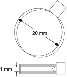 | ||
| Fig. 1 A sketch of the sample cell. The upper figure shows a view from the top, from which direction images are taken, while the lower figure is a side view. The diameter of the circular cuvette is 20 mm, and the thickness is 1 mm. | ||
III Texture dynamics: decay rates of image time-correlation functions
Right after filling the cuvette, shear-induced nematic ordering extends over very large regions with a spatial extent of the order of hundreds of microns. The extended nematic regions are induced by shear alignment due to the flow that is unavoidable when filling the cuvette. This can be seen from the left column of images of the entire cuvette in Fig. 2 as large bright regions, for various fd-concentrations. For the two lower fd-concentrations (4.0 and 11.1 mg ml−1) these large nematic domains break up into smaller domains after a few hours, as can be seen from the top-row three images on the right. In contrast, for the two higher concentrations (12.3 and 13.6 mg ml−1) the initially shear-induced large domains do not break up into smaller domains, even after extended waiting times of up to about 50–100 hours. The evolution of the images for the two higher concentrations after long waiting times, as seen in the most right bottom images in Fig. 2, is probably due to slight solvent evaporation, leading to local stress buildup, which at some point of time is released and leads to flow (this will be discussed in more detail in Section V). In the present section we will analyze the texture dynamics during break up, the dynamics once equilibrium is reached below the glass concentration, as well as the residual dynamics above the glass concentration.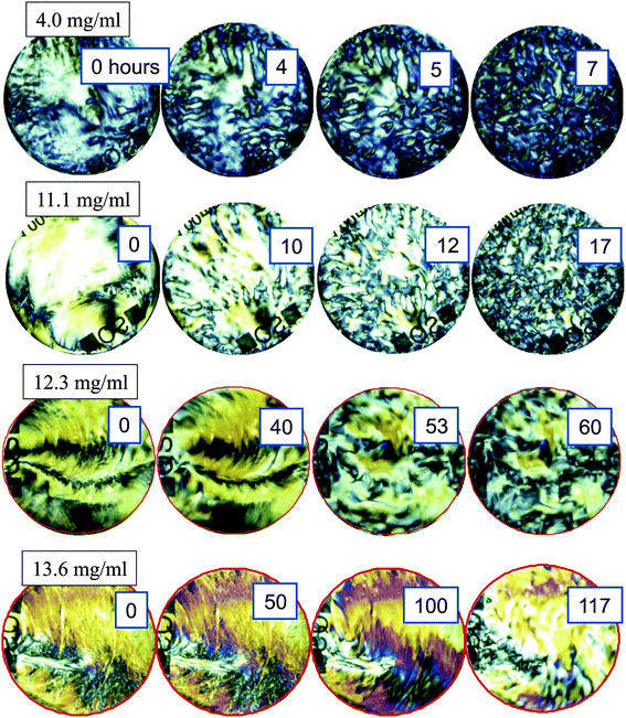 | ||
| Fig. 2 Depolarized images of the initial break up of textures as a function of fd-concentration. The concentrations of 4.0 and 11.1 mg ml−1 are below the concentration where the texture freezes, while the two higher concentrations 12.3 and 13.6 mg ml−1 are above the concentrations in the glass state. Images are taken at various waiting times, as indicated by the numbers in units of hours. | ||
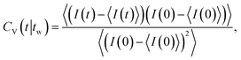
In order to quantify the dynamics of the nematic texture, we measured so-called “image time- (or video-) correlation functions” CV(t). A time series of images is recorded with the CCD camera, where images are typically taken every 10–15 minutes, over a time span of about two weeks. Let I(t) denote the transmitted intensity recorded by a single pixel on the CCD-camera chip at time t. The image-time correlation function is defined as
 | (1) |
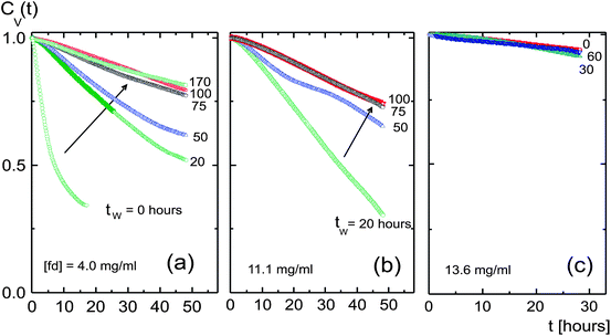 | ||
| Fig. 3 Image time-correlation functions for different waiting times tw, as indicated in the figure, for different fd-concentrations: (a) 4.0, (b) 11.1, and (c) 13.6 mg ml−1. The arrows in (a) and (b) indicate increasing waiting time for the two lower concentrations below the glass transition concentration, and (c) is above the glass concentration. | ||
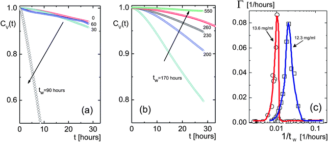
The initial decay rates for the two lower concentrations as a function of the inverse waiting time are plotted in Fig. 4. The initial decay rates of the correlation functions are relatively large right after filling the cuvette, due to the break up of the initially shear aligned poly-domains. This break up of domains is visualized in the images on the right in Fig. 4, which span an area of 7 × 7 mm2. The dynamics then significantly slows down, with a slight increase of the decay rates in the waiting-time range of about 50–80 hours. After typically 80–100 hours, the correlation functions become independent of the waiting time. At these waiting times, the transitional texture finally settles to the equilibrated state, where the decay rates are relatively small and independent of the waiting time. The plateau values of the decay rates at larger waiting times are used to characterize the dynamics of the equilibrated domain texture. Movie I in the ESI† shows the equilibration of the texture at an fd-concentration of 11.1 mg ml−1.
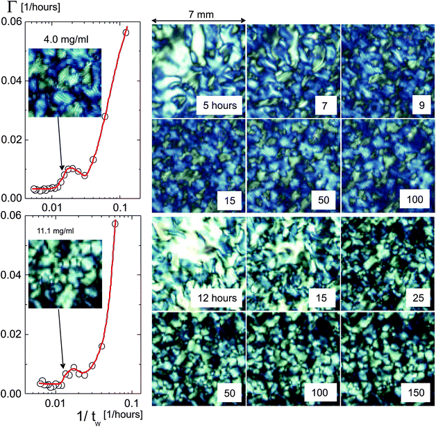 | ||
| Fig. 4 Initial decay rates of the image time-correlation functions for 4.0 mg ml−1 (upper plot), which is well below the concentration where the texture freezes, and 11.1 mg ml−1 (lower plot), which is close to that concentration, as a function of the inverse waiting time (notice the logarithmic scale). The decay rate Γ is large for short waiting times; it decreases rapidly, followed by a slight increase, after which the texture equilibrates and the decay rate attains a constant plateau value. Images of the texture morphology for several waiting times are given on the right, which span an area of 7 × 7 mm2. As can be seen from the inset images, which span an area of 3.7 × 3.7 mm2, for the lower concentration a chiral texture is formed, in contrast to the higher concentration. The arrows indicate the data point to which these images correspond. | ||
The insets in the plots on the left in Fig. 4 show a larger view of 3.7 × 3.7 mm2 of the textures. The arrows indicate the corresponding waiting time. As can be seen, a chiral texture is formed for the lower fd-concentration of 4.0 mg ml−1 (corresponding to a volume fraction of 0.0044) in contrast to the texture at the higher concentration of 11.1 mg ml−1 (a volume fraction of 0.012).
A qualitatively different behavior for the larger concentration of 13.6 mg ml−1 is observed. The decay rate is now a constant, independent of the waiting time, right from the beginning after filling the cuvette, as can be seen from the plot in Fig. 5. The images on the right in Fig. 5 confirm the very slow change of the texture, which is to be contrasted to the fast break up of the texture in Fig. 4 for the lower concentrations. The texture is now essentially frozen at this larger concentration. Moreover, the values for decay rates are now much smaller when compared to the equilibration-plateau values for the two lower concentrations.
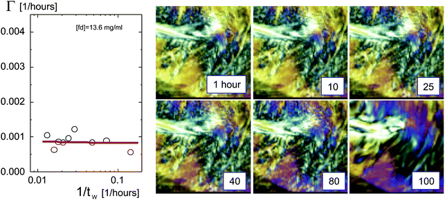 | ||
| Fig. 5 As shown in Fig. 4, but now for an fd-concentration of 13.6 mg ml−1, which is above the concentration where the texture freezes. | ||
Initial decay rates of the image correlation functions are plotted in Fig. 6 as a function of fd-concentration. For the lower concentrations the decay rates are the equilibration plateau values, and for the frozen-in texture the waiting-time-independent plateau values. There is a quite sharp change of the behavior of the texture dynamics as the concentration is increased from 11.1 to 12.3 mg ml−1. The concentration Ctext where the texture freezes is thus found to be equal to 11.7 ± 0.6 mg ml−1 (corresponding to a volume fraction of 0.013), which is within the grey area in Fig. 6. The decay rates below the freezing concentration are independent of the fd-concentration. The small, but still finite value of the decay rate above the texture-freezing concentration is due to the slow release of local stresses within the initially shear-aligned regions.
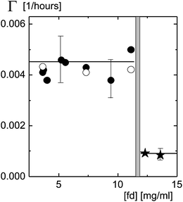 | ||
| Fig. 6 The decay rate of image time-correlation functions with a total delay-time span of 30 hours (filled circles) and 90 hours (open circles), below the texture-freezing concentration, as a function of concentration. Decay rates are measured after a waiting time of 80–100 hours. For concentrations above the texture-freezing concentration, the decay times for waiting times up to 100–150 hours are shown by the stars. | ||
IV Particle dynamics: dynamic light scattering
Dynamic light scattering (DLS) experiments measure the scattered intensity correlation function ĝT(t) = 〈i(t)i(t = 0)〉T/〈i2〉T, where i is the scattered intensity, while the brackets 〈…〉T denote averaging over the time interval over which the correlation function is recorded. The index “T” refers to the fact that a single measured correlation function is a time averaged quantity, which is different from the ensemble averaged intensity correlation function. A single, time averaged correlation function relates to a given orientation and internal structure of the domain within which the scattering volume resides. In order to obtain an ensemble averaged correlation function, averages over typically 5 to 7 correlation functions, taken at different positions in the sample, turned out to be sufficient to obtain reliable ensemble averaged correlation functions. Typical examples of time averaged intensity correlation functions for an fd-concentration of 7.3 mg ml−1 (which corresponds to a volume fraction of 0.0080) are plotted in Fig. 7a. The correlation functions in Fig. 7a are taken at different spots in the sample. The total measuring time for each function is 15 hours, so that the waiting time for each correlation function is necessarily different. Since the texture equilibrated for waiting times larger than 80–100 hours, and the measuring time is relatively short in comparison to the texture dynamics, each function corresponds to an equilibrated domain with a different orientation. The difference in domain orientation is the cause of the difference between these time-averaged correlation functions. The “brute force averaging”, in order to obtain ensemble averaged correlation functions from a series of single time averaged correlation functions, reads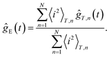 | (2) |
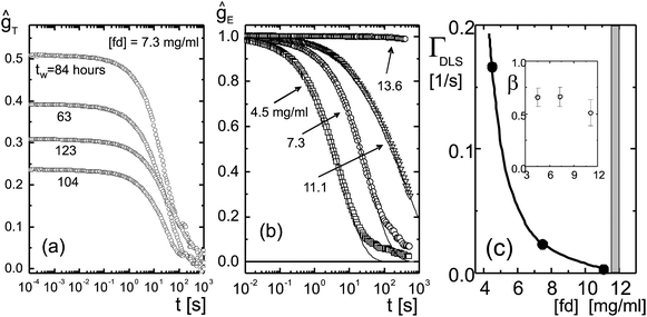 | ||
| Fig. 7 (a) Time averaged correlation functions ĝT for an fd-concentration of 7.3 mg ml−1 (a volume fraction of 0.0080), for several waiting times, as indicated in the figure. The measuring time of each function is 15 hours. (b) Ensemble averaged light scattering correlation functions for various fd-concentrations, as indicated in the figure. The solid lines are fits to a stretched exponential. (c) The inverse decay time ΓDLS = 1/τ as a function of concentration. The inset shows the fd-concentration dependence of the stretching exponent β. | ||
Duration times for the measurement of single time averaged correlation functions are typically 3 to 15 hours, during which the domain texture remains essentially unchanged. For concentrations below the concentration Ctext = 11.7 ± 0.6 mg ml−1, scattering experiments are performed after waiting times of 80–100 hours. For these waiting times an equilibrium is attained. For concentrations above the texture-freezing concentration, where the texture does not equilibrate after filling the cuvette, time averaged functions are measured also for smaller waiting times.
The wavelength of the laser beam is 633 nm, and the scattering angle is 16°, which corresponds to a length scale of 1 μm. Since the depolarized scattering of fd-virus particles is negligibly weak, correlation functions therefore probe translational displacements of the rods comparable to their length. This implies that, whenever the ensemble averaged correlation function exhibits no decay during a certain time interval, single rods are not able to diffuse over distances larger or comparable to their own length during that time. In that case the sample behaves as a glass, that is, particle motion is frozen-in during such time intervals.
Decay times larger than about 800–1000 s are at the limit of the stability of our light scattering set up. This has been verified by the measurement of correlation functions taken from a static probe (a scratched glass surface). The correlation function of such a static probe shows signs of decay at about 800 s, which is due to the limited mechanical- and laser-pointing stability.
Ensemble averaged intensity correlation functions for various fd concentrations are shown in Fig. 7b. As can be seen, particle dynamics becomes increasingly slower when the concentration is increased, and no decay of the correlation function is found for an fd-concentration of 13.6 mg ml−1 (corresponding to a volume fraction of 0.015) up to a waiting time of 100 hours. For this high fd-concentration the particle dynamics is arrested on a time scale of about 1000 s. Hence, the glass is a Wigner glass in the sense that each rod is caged by its neighbors through long ranged electrostatic interactions. This is sketched in Fig. 8, where the dotted lines indicate the extent of the electric double layer. The double layers of neighboring rods now overlap to an extent that leads to caging. At high ionic strengths, where the effective diameter of the rods is close to the very small hard-core diameter of 6.8 nm, diffusion along the long axis of the rod is essentially unhindered, so that a glass transition will not occur at realistic volume fractions. For the present thick double layers, however, the effective diameter is large, resulting in strongly hindered diffusion also along the long axis of the rods which leads to structural arrest.
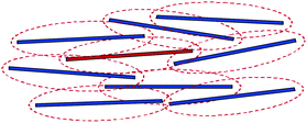 | ||
| Fig. 8 A sketch of the caging of a charged rod (in red) by its neighbors (in black), due to long ranged electrostatic repulsions. The dotted lines are used to indicate the extent of the electric double layers. | ||
The mode-coupling theory predicts that the α-mode decays like a stretched exponential exp{−(t/τ)β}. The solid lines in Fig. 7b are fits to such a stretched exponential. The slow decay for longer times seen in Fig. 7b might be due to slight rotation of domains during the measuring time of correlation functions, or might be connected to slow elastic modes. These longer times are not included in the fit to the stretched exponential. The decay rates ΓDLS = 1/τ are plotted in Fig. 7c as a function of the fd concentration, and the inset shows the value of the stretching exponent β, which attains the value of 1/2 at the glass transition with an error of about 0.10. The solid line is a guide to the eye. The grey region is the region within which the nematic texture freezes, as discussed in the previous section. The dynamical structural arrest on the particle level clearly occurs between 11.1 and 13.6 mg ml−1, which is the same range where the texture freezes. Hence, at the glass transition concentration both the dynamics at the particle level as well as the texture dynamics are arrested.
Note that there is no β-decay observed in Fig. 7a and b. The absence of the β-decay has also been reported in ref. 28. Experiments at larger scattering angles, where smaller displacements within the cage are probed, might reveal β-decay. It is feasible, however, that softer interaction potentials lead to a less pronounced β-decay due to the hindrance of motion within a cage as a result of the long-ranged repulsions. There is indeed a pronounced β-decay found in a quasi two-dimensional system of hard ellipsoids.30 Furthermore, the β-decay for hard-spheres3 is more pronounced than for micro-gel particles with a soft repulsive potential.5 The value of 0.5 ± 0.1 for the stretching exponent is within the range of what is found experimentally also for hard-sphere systems3 and for micro-gel particles5 (see their Fig. 4a, for concentrations close to the glass transition).
For the quasi two-dimensional system of ellipsoids described in ref. 30 there is no nematic state: the glass transition occurs within the isotropic state, in contrast to our findings and those described in ref. 28 for three-dimensional systems. Nevertheless there are similarities between two- and three-dimensional systems. First of all, local nematic ordering is seen within the isotropic state in the two-dimensional system described in ref. 30. Secondly, freezing of the rotational degrees of freedom is claimed to occur prior to the glass transition in the two-dimensional system. Such a “freezing” of rotational motion may be interpreted in three dimensions as being a genuine feature of a nematic state, where rotational order is also non-relaxing (apart from overall rotation of entire nematic domains). Due to the constrained motion in two dimensions, however, the detailed diffusion mechanisms in two- and three-dimensional systems near the glass transition may be quite different. A similar microscopy study of the detailed diffusion mechanisms as for a two-dimensional system in ref. 30 has not yet been undertaken for three-dimensional systems.
A surprising phenomenon is that time averaged correlation functions below the glass transition decay quite slowly for small waiting times, shortly after filling the cuvette. The correlation functions then decay much faster during equilibration, and subsequently slow down again when equilibration is reached. This can be seen in Fig. 9, where the time at which the time averaged normalized correlation functions decayed to 1/2 is plotted as a function of the waiting time. The spread in the data points in this figure reflects their reproducibility. The effect becomes more pronounced on approach of the glass transition concentration. Especially the very slow particle dynamics at small waiting times is surprising. Note that a similar non-monotonic behavior of the texture dynamics as a function of the waiting time is observed in Fig. 4. The texture decay rate for small waiting times, however, is fast, in contrast to the decay rate of the DLS correlation functions. We do not yet have an explanation for these phenomena.
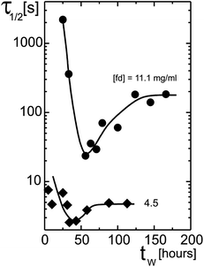 | ||
| Fig. 9 Relaxation times of time averaged correlation functions ĝT as a function of the waiting time. The decay time τ1/2 is the time at which the DLS correlation function decayed to half of its initial value. The measuring time of each separate correlation function is 5 hours for the lower concentration, and 8 hours for the higher concentration. | ||
V The onset of flow
For waiting times that are longer than those considered in the previous section on texture and particle dynamics, we observed a flow that propagates from the entrance of the cuvette into the bulk of the dispersions. Below the glass transition concentration, the onset of flow takes place at very long waiting times of 200–300 hours. For concentrations in the glass state the system is more susceptible to flow. For a concentration of 12.3 mg ml−1, just above the glass transition concentration, the flow sets in already after 30 hours, and for a concentration of 13.6 mg ml−1, deeper into the glass state, after about 60 hours. The flow is at the origin of the change of the texture as seen in the bottom-right images in Fig. 2. The onset of flow and its subsequent effect on the texture morphology can be more clearly seen in Fig. 10, where depolarized images are shown of the entire cuvette for an fd-concentration of 13.6 mg ml−1, up to waiting times of 285 hours (Movie II in the ESI shows the evolution of the morphology right from the start after filling the cuvette up to 285 hours†). Right after filling the cuvette there is an initial “streak” in the observed morphology that starts from the entrance of the cuvette (see the top-left image in Fig. 10). This streak is due to the flow that existed while filling the cuvette with a syringe. The morphology is essentially unchanged over a time span of 60 hours. After about 60 hours, a flow originates from the entrance of the cuvette that subsequently propagates into the bulk of the sample. This is especially clear from the images taken at waiting times of 117 and 133 hours in Fig. 10. At even later times the flow strongly affects the morphology, and a texture of very small domains is left after 285 hours. The most probable reason for the onset of flow is slight evaporation at the entrance of the cuvette that cannot be avoided over such long periods of time. Due to evaporation stresses build up at the entrance of the cuvette, which are released after some time, giving rise to the observed flow.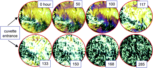 | ||
| Fig. 10 Depolarization images of the cuvette for various times, within the glass, at an fd-concentration of 13.6 mg ml−1. Flow sets in at the entrance of the cuvette. The initially shear-aligned morphology does not show a sign of relaxation before the flow sets in. | ||
The effect of flow has a pronounced effect on the image time-correlation functions, as can be seen from Fig. 11. The decay rates of the correlation function are very much enhanced once the flow sets in (see Fig. 11a). For longer waiting times the correlation functions decay slower again (see Fig. 11b). The initial slopes of the correlation functions are plotted in Fig. 11c, where the peak corresponds to the time span where the flow is visually observed. For the lower fd-concentration of 12.3 mg ml−1, just above the glass transition concentration, the flow sets in already after approximately 30 hours. For the higher fd-concentration the flow sets in after about 60 hours. The flow-induced turn-up of the decay rates with increasing waiting time is not included in the plots in Section 3 since there we are only interested in the dynamics in the equilibrated or glassy states without the perturbation of the flow. Below the glass-transition concentration the flow occurs at very long waiting times of about 300 hours.
 | ||
| Fig. 11 Correlation functions for different waiting times, as indicated in the figure, for the high concentration of 13.6 mg ml−1 (corresponding to a volume fraction of 0.015), which is above the glass transition concentration. In (a) the correlation functions are observed to rapidly decay after about 60 hours, due to the flow that emerges from the cuvette entrance (see also Fig. 10). (b) At longer times the flow probably reaches a quasi-stationary state, leading to a severe slowing down of image correlation functions. Arrows indicate increasing waiting time. (c) Decay rates for 12.3 (open squares, blue line) and 13.6 mg ml−1 (open circles, red line) for waiting times up to 400 hours. | ||
The possibility that evaporation is at the origin of the flow is confirmed by observing a droplet between two plates that is in contact with air along its entire circumference. It is indeed observed that flow sets in radially after some time from all sides of the droplet (see Movie III in the ESI†).
The fact that flow sets in much earlier in the glassy state as compared to the liquid-like state can be understood as follows. For fd-concentrations above the glass transition concentration, fd-rods are not able to diffuse into the bulk of the sample during evaporation, leading to a relatively fast build up of stresses, and a consequently relatively early occurrence of flow. Below the glass transition concentration, rods are to some extent able to diffuse into the bulk, diminishing the concentration differences at the entrance of the cuvette and the bulk. This in turn leads to a relatively long waiting time after which the flow sets in.
VI Summary and discussion
We performed experiments on suspensions of very long and thin, highly charged colloidal rods (fd-viruses) at low ionic strength, where the Debye length of 27 nm is much larger than the diameter of 6.8 nm of the core of the rods. The resulting long-ranged electrostatic interactions give rise to structural arrest above an fd-concentration of 11.7 ± 0.6 mg ml−1 (which corresponds to a volume fraction of 0.013), where each rod is caged due to a strong double-layer overlap (as sketched in Fig. 8). Structural arrest is probed by means of dynamic light scattering. The glass transition is found to occur far above the isotropic–nematic coexistence region (the lower binodal concentration is 1.5 ± 0.2 mg ml−1 and the upper binodal concentration is 3.4 ± 0.5 mg ml−1, as depicted in Fig. 12 in the lower panel). The equilibrated state is therefore a texture of either chiral nematics (see the lower two images in Fig. 12) or domains (the upper two images in Fig. 12). The domains are chiral up to 6.5 ± 0.9 mg ml−1 and a domain texture exists above that concentration. The images on the left show morphologies with a waiting time of 50 hours, while the images on the right are taken after 100 hours. Note that by using the naked eye, there is hardly any difference between the morphologies after 50 and 100 hours of waiting time. A detailed analysis by image-time correlation shows, however, that equilibration is achieved only after 80–100 hours (as indicated by the vertical grey region in Fig. 12). Initial break up of the shear-aligned domains is observed to occur within about 10 hours, slightly depending on the fd concentration (as depicted by the grey area on the left in Fig. 12). The dynamics of the texture is found to freeze at the same concentration where structural arrest occurs, as quantitatively probed by means of the image time-correlation. The decay rates of image time-correlation functions after the equilibration (below the glass transition concentration) are constant (0.0045 ± 0.00051 per hour) right up to the glass transition. There is a small but finite decay rate of the texture also above the glass transition concentration, due to the slow release of local stresses that result from shear alignment during filling of the cuvette (see Fig. 6). There are thus two features of the glass transition: structural arrest and freezing of the texture dynamics.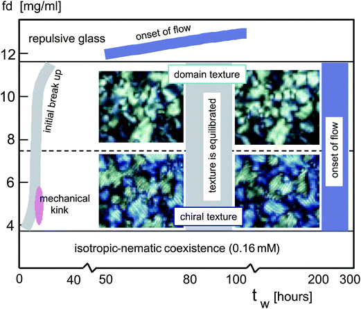 | ||
| Fig. 12 The state diagram in the fd-concentration versus waiting-time plane. Various movies are provided in the ESI.† | ||
Right after filling the cuvette, for small waiting times, a fast decay of image time-correlation functions is found. The decay slows down for longer waiting times, followed by a transient faster decay, before an equilibrium is reached, where the decay rates are significantly smaller as compared to the fast initial rates (see Fig. 4). For the particle dynamics as probed by dynamic light scattering, however, the relaxation times of correlation functions are initially very large, then become smaller, and go through a minimum before reaching equilibrium (see Fig. 9). This phenomenon is more pronounced close to the glass transition concentration.
At quite low concentrations (between 4.5 and 5.6 mg ml−1), we observed in the early stage of equilibration (typically around waiting times of 10–15 hours) a “mechanical kink” (see the pink area in Fig. 12). Here, the entire texture is shifted/rotated over a small distance/angle in a discontinuous fashion at a certain instant of time, without a change of the overall structure of the domain texture. This can be seen in Movie IV in the ESI.† The interpretation of this sudden change is that during equilibration stresses accumulate throughout the sample, which are released after a certain waiting time.
After extended waiting times, we observed a disruption of the domain texture (see Movies II and III in the ESI†). The flow is observed after 200–300 hours below the glass transition concentration (see the blue vertical region on the right in Fig. 12). In the glass, however, the flow sets in at much earlier times (see the blue inclined line at the top in Fig. 12). The flow is caused by solvent evaporation at the entrance of the cuvette. After very long times (about 300–500 hours), the decay rates of image time-correlation functions become smaller than those in the frozen state, before flow occurred (see Fig. 11a and b).
References
- P. N. Pusey and W. van Megen, Nature, 1986, 320, 340 CrossRef CAS.
- W. van Megen and P. N. Pusey, Phys. Rev. A, 1991, 43, 5429 CrossRef CAS.
- W. van Megen and S. M. Underwood, Phys. Rev. E: Stat. Phys., Plasmas, Fluids, Relat. Interdiscip. Top., 1994, 49, 4206 CrossRef CAS.
- W. van Megen, T. C. Mortensen and S. R. Williams, Phys. Rev. E: Stat. Phys., Plasmas, Fluids, Relat. Interdiscip. Top., 1998, 58, 6073 CrossRef CAS.
- E. Bartsch, M. Antonietti, W. Schupp and H. Sillescu, J. Chem. Phys., 1992, 97, 3950 CrossRef CAS.
- Ch. Beck, W. Härtl and R. Hempelmann, J. Chem. Phys., 1999, 111, 8209 CrossRef CAS.
- J. Stellbrink, J. Allgaier and D. Richter, Phys. Rev. E: Stat. Phys., Plasmas, Fluids, Relat. Interdiscip. Top., 1997, 56, R3772 CrossRef CAS.
- D. Vlassopoulos, J. Polym. Sci., Part B: Polym. Phys., 2004, 42, 2931 CrossRef CAS.
- C. Mayer, E. Zaccarelli, E. Stiakakis, C. N. Likos, F. Sciortino, A. Munam, M. Gauthier, N. Hadjichristidis, H. Iatrou, P. Tartaglia, H. Löwen and D. Vlassopoulos, Nat. Mater., 2008, 7, 780 CrossRef CAS.
- D. Vlassopoulos and G. Fytas, Adv. Polym. Sci., 2009, 236, 1 CrossRef.
- W. C. K. Poon, J. Phys.: Condens. Matter, 2002, 14, R859 CrossRef CAS.
- W. Götze and L. Sjögren, Rep. Prog. Phys., 1992, 55, 241 CrossRef.
- W. Götze, Complex Dynamics of Glass-Forming Liquids - A Mode-Coupling Theory, Oxford University Press, New York, 2009, vol. 143 Search PubMed.
- W. van Megen, T. C. Mortensen and S. R. Williams, Phys. Rev. E: Stat. Phys., Plasmas, Fluids, Relat. Interdiscip. Top., 1998, 58, 6073 CrossRef CAS.
- W. K. Kegel and A. van Blaaderen, Science, 2000, 287, 290 CrossRef CAS.
- E. R. Weeks, J. C. Crocker, A. C. Levitt, A. Schofield and D. A. Weitz, Science, 2000, 287, 627 CrossRef CAS.
- E. Donth, The Glass Transition: Relaxation Dynamics in Liquids and Disordered Materials, Springer, Berlin, 2001 Search PubMed.
- W. van Megen, J. Phys.: Condens. Matter, 2002, 14, 7699 CrossRef CAS.
- C. A. Angel, MRS Bull., 2008, 33, 544 CrossRef.
- H. Tanaka, J. Stat. Mech.: Theory Exp., 2010, 12, 12001 CrossRef.
- M. J. Solomon and P. T. Spicer, Soft Matter, 2010, 6, 1391 RSC.
- L. Berthier and G. Biroli, Rev. Mod. Phys., 2011, 83, 587–645 CrossRef CAS.
- C. Donati, J. F. Douglas, W. Kob, S. J. Plimpton, P. H. Poole and S. C. Glotzer, Phys. Rev. Lett., 1998, 80, 2338 CrossRef CAS.
- R. C. Kramb, R. Zhang, K. S. Schweizer and C. F. Zukoski, Phys. Rev. Lett., 2010, 105, 055702 CrossRef CAS.
- P. Pfleiderer, K. Milinkovic and T. Schilling, Europhys. Lett., 2008, 84, 16003 CrossRef.
- C. F. Schreck, M. Mailman, B. Chakraborty and C. S. O'Hern, Phys. Rev. E: Stat. Phys., Plasmas, Fluids, Relat. Interdiscip. Top., 2012, 85, 061305 CrossRef.
- C. F. Schreck, N. Xu and C. S. O'Hern, Soft Matter, 2010, 6, 2960 RSC.
- A. Wierenga, A. P. Philipse and H. N. W. Lekkerkerker, Langmuir, 1998, 14, 55 CrossRef CAS.
- K. Kang and J. K. G. Dhont, Phys. Rev. Lett., 2013, 110, 015910 CrossRef.
- Z. Zheng, F. Wang and Y. Han, Phys. Rev. Lett., 2011, 107, 065702 CrossRef.
- E. Weeks, Physics, 2011, 4, 61 CrossRef.
- Y. Y. Huang, S. V. Ahir and E. M. Terentjev, Phys. Rev. B: Condens. Matter, 2006, 73, 125422 CrossRef.
- G. M. H. Wilkins, P. T. Spicer and M. J. Solomon, Langmuir, 2009, 25, 8951 CrossRef CAS.
- A. J. W. ten Brinke, L. Bailey, H. N. W. Lekkerkerker and G. C. Maitland, Soft Matter, 2007, 3, 1145 ( Soft Matter , 2008 , 4 , 337 ) RSC.
- O. Henrich, A. M. Puertas, M. Sperl, J. Baschnagel and M. Fuchs, Phys. Rev. E: Stat. Phys., Plasmas, Fluids, Relat. Interdiscip. Top., 2007, 76, 031404 CrossRef CAS.
- R. Schilling and T. Scheidsteger, Phys. Rev. E: Stat. Phys., Plasmas, Fluids, Relat. Interdiscip. Top., 1997, 56, 2932 CrossRef CAS.
- M. Letz, R. Schilling and A. Latz, Phys. Rev. E: Stat. Phys., Plasmas, Fluids, Relat. Interdiscip. Top., 2000, 62, 5173 CrossRef CAS.
- C. De Michele, R. Schilling and F. Sciortino, Phys. Rev. Lett., 2007, 98, 265702 CrossRef.
- Z. Dogic and S. Fraden, Langmuir, 2000, 16, 7820–7824 CrossRef CAS.
- E. Grelet and S. Fraden, Phys. Rev. Lett., 2003, 90, 198302 CrossRef.
- Z. Dogic and S. Fraden, Philos. Trans. R. Soc., A, 2001, 359, 997–1015 CrossRef CAS.
- S. Fraden, Phase transitions in Colloidal Suspensions of Virus Particles, in Observation, Prediction and Simulation of Phase Transitions in Complex Fluids, ed. M. Baus, L. F. Rull and J. P. Ryckaert, Kluwer Academic Publishers, Dordrecht, 1995, vol. 460, NATO-ASI-Series C, p. 113 Search PubMed.
- K. Zimmermann, J. Hagedorn, C. C. Heuck, M. Hinrichsen and J. Ludwig, J. Biol. Chem., 1986, 261, 1653 CAS.
- K. Kang, A. Wilk, A. Patkowski and J. K. G. Dhont, J. Chem. Phys., 2007, 126, 214501 CrossRef.
- K. Kang, Rev. Sci. Instrum., 2011, 82, 053903 CrossRef.
Footnote |
| † Electronic supplementary information (ESI) available: Four movies. See DOI: 10.1039/c3sm27754b |
| This journal is © The Royal Society of Chemistry 2013 |